Abstract
Diffraction-based velocity analysis is a key data interpretation technique in geophysical exploration, typically relying on the geometric characteristics, energy distribution, or propagation paths of diffraction waves. The hyperbola-based method is a classical strategy in this category, which extracts depth-dependent velocity (or dielectric properties) by correlating the hyperbolic shape of diffraction events with subsurface parameters for characterizing subsurface structures and material compositions. In this study, we propose a layer-stripping velocity analysis method applicable to ground-penetrating radar (GPR) and lunar-penetrating radar (LPR) data, with two main innovations: (1) replacing traditional local optimization algorithms with an intuitive parallelism check scheme, eliminating the need for complex nonlinear iterations; (2) performing depth-progressive velocity scanning of radargram diffraction signals, where shallow-layer velocity analysis constrains deeper-layer calculations. This strategy avoids misinterpretations of deep geological objects’ burial depth, morphology, and physical properties caused by a single average velocity or independent deep-layer velocity assumptions. The workflow of the proposed method is first demonstrated using a synthetic rock-fragment layered model, then applied to derive the near-surface dielectric constant distribution (down to 27 m) at the Chang’e-4 landing site. The estimated values range from 2.55 to 6, with the depth-dependent profile revealing lunar regolith stratification and interlayer material property variations. Consistent with previously reported results for the Chang’e-4 region, our findings confirm the method’s applicability to LPR data, providing a new technical framework for high-resolution subsurface structure reconstruction.
1. Introduction
Velocity analysis plays a crucial role in geophysical exploration, serving as the key step for converting “surface signals” into “subsurface structural models”. By precisely determining the propagation velocity of wavefields in subsurface media, this technique ensures the reliability of inversion imaging and mitigates the non-uniqueness in geological interpretation.
Velocity analysis traces its origins to seismic exploration. Owing to the strong amplitudes, continuous events, and high signal-to-noise ratios of reflected waves in seismic records, reflection-based velocity analysis has emerged as the dominant approach for conventional seismic surveys. However, reflected waves are highly dependent on continuous subsurface interfaces and exhibit weak responses to small-scale discontinuities and heterogeneous media, presenting a major challenge for constructing accurate velocity models. In contrast, although diffraction waves are inherently weaker in amplitude, they can effectively delineate subsurface discontinuities (e.g., fault endpoints, stratigraphic pinch-outs, small lenses, and cavities). This unique attribute enables diffraction-based velocity analysis to achieve precise spatial localization, provide robust constraints on local velocities, and thereby minimize errors in structural modeling. In recent years, substantial progress has been made in the research of diffraction-based velocity analysis and migration imaging, establishing a solid foundation for its practical application in complex geological settings [1,2,3,4,5].
In ground-penetrating radar (GPR) investigations, an accurate dielectric constant model is crucial for high-resolution imaging and reliable characterization of subsurface properties. The relationship between the propagation velocity of electromagnetic (EM) waves in subsurface media (e.g., rocks and soils) and dielectric constant is defined as follows:
where denotes the propagation velocity of the EM waves, is the relative dielectric permittivity, and represents the speed of light in free space [6].
Equation (1) allows seismic velocity analysis methods to be directly applied to the processing and interpretation of GPR data, thus supporting the identification and reconstruction of complex subsurface electrical structures. Current velocity modeling techniques for GPR data primarily fall into two categories: migration-based approaches and hyperbola analysis. The former estimates velocities by exploiting differences in the focusing of diffraction events under varying migration velocities [7,8,9], while the latter relies on hyperbolic fitting to deduce velocities/dielectric constants from the hyperbolic signatures of subsurface targets in GPR B-scan profiles. In the context of hyperbola-based methods (HBMs), ref. [10] proposed a high-resolution velocity estimation framework for common-offset GPR data, which first retrieves the smooth, large-scale velocity components through diffraction analysis and subsequently resolves superimposed small-scale fluctuations via reflection waveform inversion. Ref. [11] further advanced this direction by developing an algorithm for the automated detection and picking of hyperbolic diffraction events, which was successfully applied to map EM velocity distributions from glacier GPR datasets. Beyond general velocity estimation, researchers have also tailored HBMs for specific applications. For example, in nondestructive testing and municipal infrastructure surveys, an integrated algorithm combining circular and hyperbolic formulations has been developed to process ground-coupled GPR data, enabling the simultaneous estimation of subsurface dielectric constant distributions and key geometric parameters of buried pipelines, such as radius and depth [12,13].
In recent years, velocity analysis has been widely used in lunar and planetary GPR studies. Its objective is to reconstruct subsurface velocity structures to obtain: (1) depth information in radargrams (e.g., layer depth, thickness, and dip angle); and (2) quantitative parameters of material properties. For instance, variations in dielectric constant can be quantified using Equation (1) and further converted to rock bulk density [14].
where denotes the rock bulk density (units: or ), is the logarithm of the relative permittivity, and serves as a normalization factor to ensure consistency in both the units and order of magnitude.
This information is crucial for revealing the material composition, evolutionary history, and potential resource distribution of planetary bodies. The HBMs have been extensively used in this field, as hyperbola matching is the only approach for permittivity estimation that is monostatic, single-offset, purely GPR-based, and independent of a priori depth information or amplitude inversion. For example, to estimate the dielectric properties of the lunar regolith at the Chang’e-3 landing site, ref. [15] applied the direct least-squares method to fit hyperbolic equations to discrete data points. Ref. [16] derived velocity by combining local correlation with similarity analysis of Lunar Penetrating Radar (LPR) data. Ref. [17] also used an HBM to extract parabolic-shaped diffractions (PSDs) from LPR data to obtain the dielectric constant and the density profiles with depth. By accounting for the height of the radar antenna, ref. [18] enhanced the dielectric constant inversion method based on PSD analysis. Building on this, ref. [19] further incorporated antenna spacing to improve the geometric modeling accuracy of the method. Moreover, HBMs have also been successfully applied to estimate dielectric constant distributions from Martian GPR data [20,21,22,23].
However, most HBMs treat the hyperbolic-shaped diffractions at different depths as mutually independent, neglecting the physical inheritance and gradual variation of subsurface properties across layers. This simplification can lead to deviations from the true velocity structure. To address this limitation, we propose a layer-stripping velocity analysis method that sequentially estimates velocities for all hyperbolic-shaped diffractions from shallow to deep based on the arrival times of their apexes. In this process, velocity values estimated from shallow layers are used to constrain the scanning of deeper layers. Furthermore, by adopting a “parallelism check” strategy for characteristic points, we iteratively refine the velocity estimates until these points achieve optimal parallelism or overlap with the simulated travel-time curves, thus yielding accurate velocity estimates. The proposed method is validated using a synthetic layered model embedded with rock fragments, and is further applied to LPR data acquired during the first four lunar days of the Chang’e-4 mission to reconstruct the subsurface dielectric permittivity profile for the landing site.
2. Methodology
GPR transmits carrier-free electromagnetic pulses into the subsurface. Due to the spherical wavefronts emitted by the GPR antenna, reflections occur not only when the antenna is directly above a target but also as it moves nearby. Consequently, the varying distance between the antenna and the target causes the recorded reflections to form characteristic diffraction hyperbolas in the radargram [24]. This detection mechanism is illustrated in Figure 1.
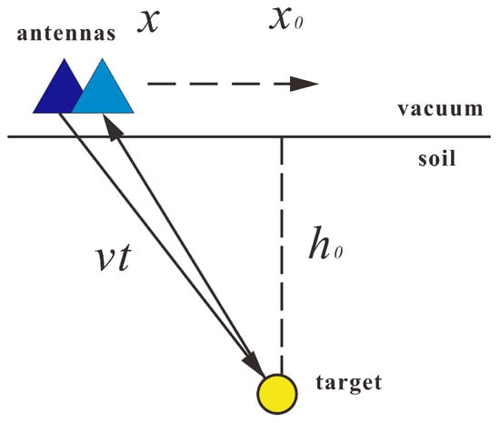
Figure 1.
Schematic diagram of GPR detection.
Given the irregular geometries of most subsurface rocks and the decreasing influence of rock diameter with depth, we approximate subsurface targets as point reflectors to simplify the forward modeling. Based on the analysis of EM wave propagation paths, the geometric relationship between diffraction hyperbolas and the estimated parameters can be explicitly defined. As shown in Figure 1, for a given antenna position x (m), the distance from its center to the point reflector is expressed as , where t denotes the total two-way travel time and represents the average EM wave propagation velocity in the medium. When the antenna is located directly above the vertical axis of the point reflector (i.e., ), this distance corresponds to the target depth . Since this geometric configuration forms a right triangle, the following functional relationship can be established:
Each set of raw data points extracted from the diffraction hyperbola of a single point reflector satisfies Equation (4):
Equation (4) can be rearranged as its canonical hyperbolic form:
where the semi-major and semi-minor axes of the hyperbola are expressed as:
The shape of the hyperbola or the angle between its asymptotes can be quantified using Equations (6) and (7):
Evidently, the asymptote angle is directly proportional to the average EM wave propagation velocity .
The conventional hyperbolic fitting method typically begins by either manually or automatically identifying hyperbolas corresponding to different diffraction events in the radargram; next, extracting the observed data points from each hyperbola segment; finally, applying a direct least-squares method to estimate the optimal parameters , a, and b, subject to the following condition:
Subsequently, we can calculate the depth of different subsurface rock fragments, as well as the EM wave propagation velocity . Key advantages of this approach include its high computational efficiency, suitability for linearizing nonlinear problems, and capability for rapid velocity model estimation.
In contrast to the method described above, this paper proposes a relatively novel velocity-scanning approach. In this approach, prior to analyzing the velocity of each diffraction event, three characteristic points (i.e., the apex and one point on each flank) are first selected from the recorded hyperbolic signature. An initial velocity is assumed and treated as a known value. Following this, a series of diffraction reference points are placed along the vertical axis of the reflector to compute the simulated travel-time curves (hereafter referred to as “theoretical hyperbolas”) corresponding to wavefields propagating upward to the ground surface.
As indicated by Equation (8), the asymptote angle is related to the velocity. Building on this, we propose a “parallelism check” scheme that evaluates the validity of the currently assumed velocity by examining the positional relationship between the selected characteristic points and the asymptotes of the “theoretical hyperbolas”. Specifically, if the characteristic points are parallel to the adjacent “theoretical hyperbolas”, this indicates that the asymptote angles of the “actual hyperbola” and “theoretical hyperbolas” are identical, confirming the accuracy of the assumed velocity (Figure 2b). Conversely, if intersections occur, the asymptotic angles of these two hyperbolas are inconsistent, indicating that the assumed velocity is inaccurate (Figure 2a). This necessitates reassigning a new value to and repeating the above comparison iteratively until parallelism is achieved, from which the true propagation velocity can be derived. Furthermore, a layer-stripping strategy is incorporated into the proposed method. This strategy performs a sequential shallow-to-deep velocity scan for all identified diffraction events in the record. Crucially, the velocity analysis of deeper layers fully accounts for the effects of shallow ones, thus avoiding errors associated with using a single average velocity or treating deep-layer velocities in isolation.
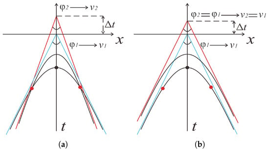
Figure 2.
Positional relationship between characteristic points and the theoretical hyperbola. (a) Parallel alignment; (b) Intersecting case.
The proposed method is implemented through the following sequential steps:
Step 1. Input and adjust travel time: Convert the two-way travel time t from the original radargram records to the one-way travel time .
Step 2. Pick and number diffraction events: Manually select diffraction waves with well-defined hyperbolic shapes, then number them sequentially according to the increasing arrival time of their apexes.
Step 3. Select the current target: Begin with the diffraction event with the smallest number (i.e., the shallowest target), followed by extracting three key characteristic points (i.e., the apex and one point on each flank) from its recorded segment.
Step 4. Assign velocity and convert time-to-depth: Assign an initial assumed velocity greater than the possible maximum in the study area. If overlying layers exist, incorporate their velocities to convert the current apex’s one-way travel time to depth (target’s maximum depth); for the first layer, perform the conversion directly using the assumed velocity.
Step 5. Compute simulated travel-time curves: Place equally spaced “reference point sources” above the current diffraction apex (at horizontal position ) down to the maximum depth. Calculate their travel-time curves to the surface using the Fast Marching Method (FMM) based on wavefront propagation, incorporating velocities from both the overlying and current layers [25,26,27].
Step 6. Compare and optimize: Compare the positions of the three characteristic points from Step 3 against the simulated travel-time curves obtained in Step 5.
Step 7. Determine the bottom interface of the current layer: Use the “true velocity” identified in Step 6 to recalculate the depth of the current diffraction apex and designate this depth as the bottom interface of the current layer (i.e., the actual burial depth of the target).
Step 8. Iterate to build the model: Repeat Steps 3–7 sequentially for all numbered diffraction events to progressively build a layered velocity model. The velocity below the base of the model defaults to the value of the lowermost layer.
Step 9. Derive the permittivity model: Convert the final velocity model from Step 8 into a relative permittivity model with Equation (1), applying moderate smoothing as necessary to ensure continuity.
To intuitively visualize its logical structure and inter-step dependencies, the aforementioned implementation workflow is summarized in the following flowchart (Figure 3).
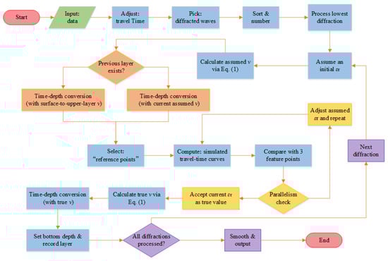
Figure 3.
Implementation flowchart of the layer-stripping velocity analysis.
3. Model Testing
In this section, we used a layered medium model containing rock fragments (Figure 4) to generate synthetic GPR data. This numerical experiment was designed to illustrate the implementation of the proposed method and to validate its feasibility. The model incorporates both the random distribution of rock fragments and the stratified nature of the subsurface medium. For simplicity, rock fragments are approximated as point scatterers in the simulation. It is worth noting that a dielectric permittivity model, rather than a velocity model, is provided directly here. This is primarily because dielectric permittivity is the key parameter governing EM wave propagation in the medium. Consequently, the method proposed in Section 2 can also be interpreted as an approach for dielectric permittivity estimation in GPR applications.
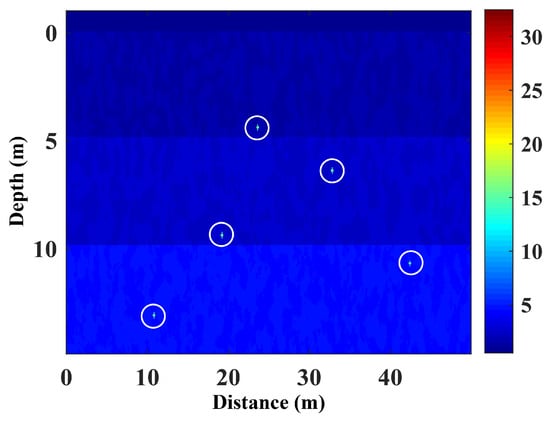
Figure 4.
A layered medium model with rock fragments.
The model dimensions are , with a top air layer of m. EM wave propagation in this stratified medium was simulated using the finite-difference time-domain (FDTD) method. Specifically, we adopted MATLAB R2024b codes [28] to generate synthetic surface-based reflection GPR data, formulated in a transverse magnetic (TM-) mode. The FDTD spatial grid was set to , resulting in a total of 80,000 grid points. The model consists of three horizontal layers: layer 1 (), with a relative permittivity of ; layer 2 (), ; layer 3 (), . Five cross-shaped scatterers with (highlighted with white circles) were randomly distributed across different layers at the following coordinates: , , , , and . Each scatterer extends laterally and vertically over two grid intervals.
The surface acquisition system was configured in a common-offset geometry, comprising an array of 497 antennas (including both transmitters and receivers). For each transmitter, the emitted signal was recorded by three adjacent receivers. A Gaussian wavelet with a central frequency of 150 MHz was used as the input source, which was assumed to be known. The sampling interval was 0.5 ns. After converting the two-way travel time to one-way travel time, the original simulated GPR record (T = 300 ns) was truncated to 150 ns, as shown in Figure 5. This adjustment was necessary primarily because, in a common-offset system, the two-way travel time includes the round-trip path difference of EM waves. This effect introduces more significant curvature variations in the diffraction hyperbolas, which would otherwise complicate the identification of characteristic points and the application of the “parallelism check” scheme.
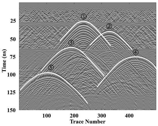
Figure 5.
Radargrams with numbered identifiable diffraction hyperbolas.
Since the randomly distributed scatterers in the layered model are slightly smaller than or comparable to the wavelength of the incident EM waves, the diffraction waves in the GPR profile exhibit high-curvature interfaces. The white hyperbolas in Figure 5 indicate the identifiable diffraction events, which correspond to the five embedded scatterers. These events were then sorted in ascending order of their apex arrival times and labeled sequentially as ①, ②, ③, ④, and ⑤. Three characteristic points were extracted from the record segment of each diffraction event.
Next, the unprocessed diffraction event with the smallest apex travel time was selected for processing and denoted as (i = 1, 2, 3, 4, 5). An assumed was assigned to the current layer, chosen to be lower than the pre-determined minimum relative permittivity of the study area. Taking diffraction event ① as an example, the minimum relative permittivity of Layer 1 is ; therefore, the assumed value was set to . According to Equation (1), this assumed corresponds to a velocity greater than the maximum of the model. Using the velocities of the overlying layers (derived from their known permittivity values), we performed time-to-depth conversion on the currently processed hyperbola, yielding the maximum possible depth of the target. Since diffraction event ① was located within Layer 1, its time-to-depth conversion was implemented directly with the assumed of the current layer.
Then, between this depth and the surface, a set of evenly spaced points is positioned along the vertical line directly above the apex of the hyperbola ①. These points served as potential source locations for generating the diffraction signal (Figure 6). We next computed the travel time curves for each reference point source through the FMM, incorporating both the assumed permittivity of the current layer and the known permittivity of overlying layers (Figure 7).
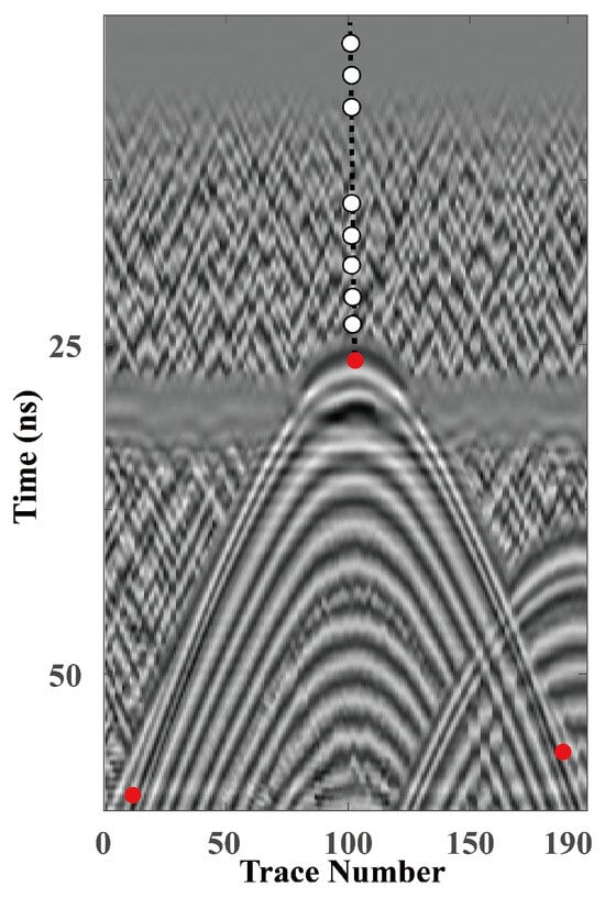
Figure 6.
Minimum-apex-travel time diffraction event and its overlying reference point sources.
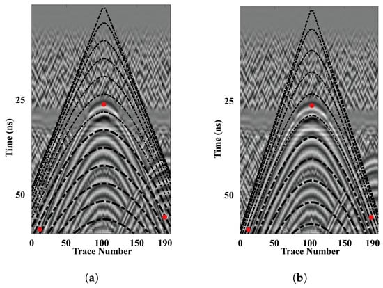
Figure 7.
Traveltime curves of the respective reference point sources. (a) For ; (b) For .
Next, we applied the “parallelism check” scheme described in Section 2 to evaluate the spatial relationship between the three characteristic points of the processed diffraction event ① and the surrounding simulated travel time curves. As illustrated in Figure 7a, when the assumed relative permittivity was set to , the three points intersected the adjacent simulated travel time curves, indicating a lack of parallelism. We therefore adjusted from 2 to 3 and recalculated the travel time curves for further comparison. Figure 7b shows that the three points became parallel to the adjacent simulated travel time curves after adjustment, confirming as the true relative permittivity of the current layer. Using this value, we re-conducted time-to-depth conversion on diffraction event ①, with the resulting depth defined as the bottom interface of the current layer (denoted as ). Theoretically, the number of identified layers should be consistent with the number of extracted diffraction events.
Finally, the five extracted diffraction events were processed sequentially to reconstruct a complete layered dielectric permittivity model. As shown in Figure 8a (blue solid line), the scatterer-based velocity analysis method accurately recovers the dielectric permittivity values of each layer. Moreover, the estimated layer depths show excellent agreement with the true model and are slightly affected by the high-permittivity objects within the layers. To suppress the “discrete step artifacts” introduced by the proposed method, we adopted an iterative smoothing algorithm based on anisotropic diffusion, governed by the following equations:
where denotes the diffusion step size, and represents the gradient sensitivity coefficient. This algorithm adaptively modulates the smoothing intensity according to local velocity gradients, thereby effectively preserving the structural details of the model. Here, was set to 0.3, to 0.05, and the number of iterations to 120.
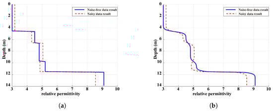
Figure 8.
Velocity analysis results for dielectric permittivity. (a) Derived layered dielectric permittivity model; (b) Moderately smoothed version of (a).
The smoothed results are presented in Figure 8b (blue solid line), which demonstrates that key features (e.g., inflection points and layer interfaces) are well retained, making the model more compatible with the gradual variation characteristics of subsurface media. To further evaluate the robustness of the proposed approach against noisy data, a numerical test was performed using synthetic GPR data corrupted with 25% Gaussian white noise, simulating the interference commonly encountered in field GPR surveys. Following the same processing workflow applied to the noise-free data, the results before and after smoothing were denoted by the red dashed lines in Figure 8a and Figure 8b, respectively.
It can be observed that the noise-contaminated results (red dashed lines) show slight deviations from the noise-free references (blue solid lines) at multiple depth intervals (e.g., 5–10 m), which reflects the influence of Gaussian noise on the velocity analysis. Nonetheless, the overall trend (i.e., the step-like variations of with depth) remains highly consistent between the two profiles. To quantify the discrepancy, the Mean Absolute Error (MAE) was calculated using Equation (11):
Here, N denotes the total sampling points, and represent the relative permittivity values at the i-th point for the noisy and noise-free results, respectively.
The calculated MAE is 0.2861. Given that the background values of the model range from 3 to 9, this MAE accounts for approximately 4.8% of the total variation in permittivity. This quantitative result demonstrates that, even under 25% Gaussian white noise, the retrieved model is minimally affected by noise, with its distribution trends fully preserved. These findings confirm that the layer-stripping velocity analysis method exhibits strong noise resistance, maintaining both the accuracy and reliability of model reconstruction.
4. Field Data Testing
To evaluate the performance of the proposed method on field data, we applied it to the LPR data acquired during the first four lunar days of the Chang’e-4 (CE-4) mission. As the first human-made spacecraft to achieve soft landing and roving exploration on the far side of the Moon, the CE-4 probe consists of a lander and the Yutu-2 rover, designed to characterize the subsurface structure and regolith properties of the landing area. To balance penetration depth and range resolution of radargrams, the CE-4 LPR adopts the same dual-channel configuration as the CE-3 LPR, with center frequencies and bandwidths of 60 MHz/40 MHz (Channel-I) and 450 MHz/500 MHz (Channel-II) [15,29,30]. Specifically, Channel-II is dedicated to shallow lunar regolith exploration, using one transmitting antenna and two receiving antennas with different offsets (denoted as CH-2A and CH-2B).
We selected LPR data for validation for two principal reasons: (1) The lunar regolith contains widely distributed inhomogeneities (e.g., boulders and voids) that act as scatterers, generating diffraction hyperbolas with distinct and identifiable shapes in radargrams; (2) The LPR system can be approximated as a zero-offset configuration, thus, velocity modeling for LPR data relies primarily on fitting discrete diffraction hyperbolas, which aligns with the core technique of the proposed method.
Prior to its restart on the fifth lunar day (29 May 2019), the Yutu-2 rover had accumulated a total driving distance of 178.9 m ([17]; Figure 9). Upon awakening each lunar day, it initiates LPR data acquisition along the entire traverse path. To ensure data quality, we excluded data collected when the rover was stationary or moving at very low speeds. Ultimately, a total of 5895 high-quality Channel-II traces were selected from the data between waypoints X and LE402 to construct a continuous profile by integrating multiple data segments (Figure 10). Due to signal attenuation and increasing noise with depth, data within the time window of 500–640 ns were discarded.
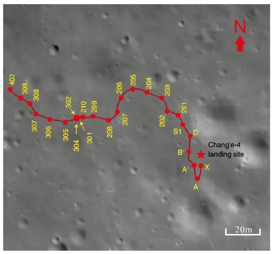
Figure 9.
The track of the Yutu-2 rover on the lunar surface. The CE-4 lander position is marked by a red star. The red line traces the rover’s path of 178.9 m across 26 waypoints (red dots) from location X to 402 during the first four lunar days. Red dots at waypoints S1, 210, 309, and 402 indicate the locations where the rover hibernated for the lunar night, on 30 January, 28 February, 29 March, and 29 April 2019, respectively. The image was captured by the CE-4 landing camera, with its left portion occluded by the lander.
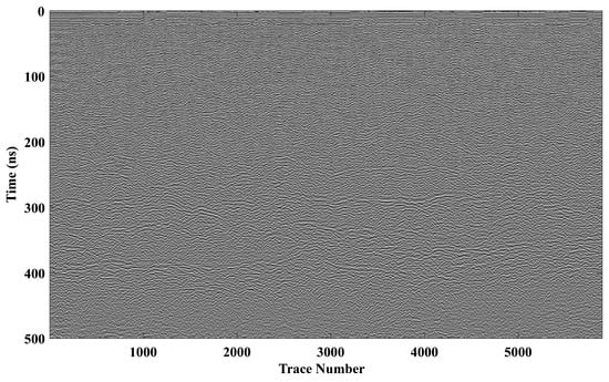
Figure 10.
Channel-II radargram of CE-4 LPR.
To implement the proposed velocity/dielectric permittivity estimation, the initial step involves identifying hyperbolic diffraction patterns within the LPR radargrams. A variety of automatic diffraction detection methods have been developed, including classical algorithms (e.g., the Hough transform [31]) and machine-learning-based approaches (e.g., pattern recognition using neural networks and support vector machine classifiers [32,33,34]). The former relies on a predefined hyperbolic model, which often fails to adequately characterize real lunar regolith conditions, leading to identification inaccuracies. The latter requires large-scale annotated datasets; however, high-quality “diffraction-background” labels in LPR images are scarce, and biased or unrepresentative training samples impair the generalization ability of the model, resulting in significant performance degradation in new survey areas. Therefore, we opted to manually pick the diffraction hyperbolas.
During the identification process, we first selected hyperbolic patterns with strong amplitudes, high curvature, and clear distinctiveness, followed by rigorous screening to eliminate false positives (e.g., secondary hyperbolas produced by buried scatterers or noise-induced pseudo-hyperbolas). The 31 manually identified hyperbolas are marked by white solid lines in Figure 11, each indicating a potential void or buried boulder within the lunar regolith. These hyperbolas are distributed across both shallow and deep regions of the radargram and are numbered in ascending order of apex travel time.
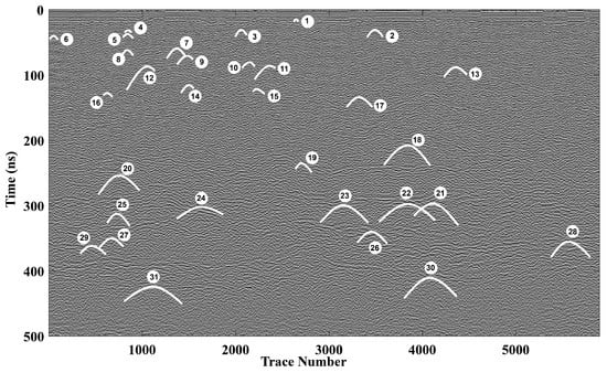
Figure 11.
Diffraction hyperbolas identified in the LPR profile.
Following the procedure outlined in Section 2, we first extracted the data segment of each diffraction event and then selected its three characteristic points. It should be noted that LPR field data often contain considerable clutter and noise around the hyperbolas, which may interfere with the extraction of characteristic points. Therefore, the following principles should be followed: (1) The true apex must lie on the symmetry axis of the hyperbola and generally corresponds to the strongest and most continuous signal peak. It is crucial to avoid mistaking high-amplitude noise artifacts for the apex; (2) The two flank reference points should preferably be selected from regions with continuous, amplitude-stable hyperbolic signals and must be symmetrically distributed relative to the apex. The three red spots in Figure 12 illustrate the characteristic points selected for diffraction hyperbola #1 according to these criteria.
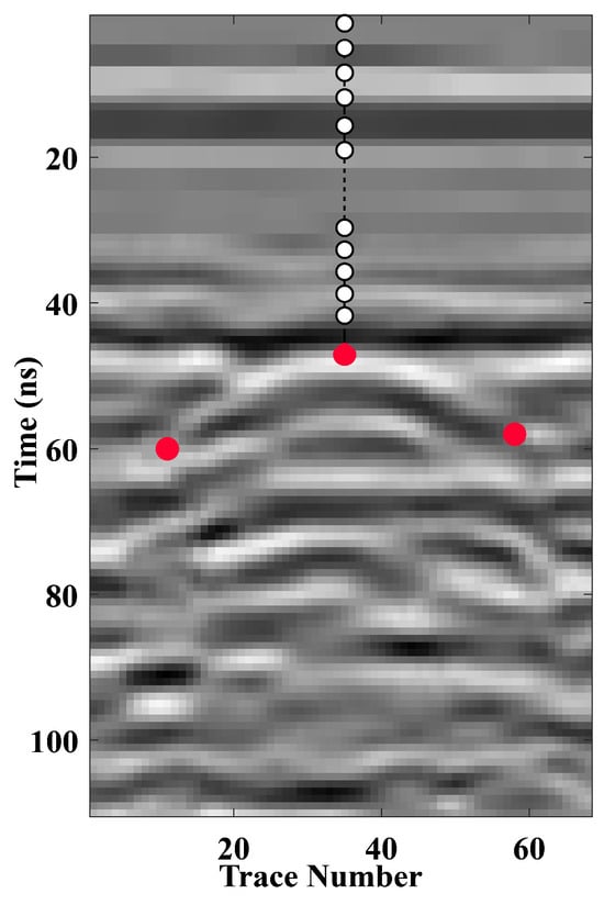
Figure 12.
Characteristic points and overlying reference points of diffraction hyperbola #1.
Next, diffraction hyperbola #1 was used to demonstrate the implementation of the proposed method on field data. As hyperbola #1 has the smallest apex travel time, we first assigned an assumed relative permittivity for the first layer, which is lower than the minimum in the study area. Based on the published analysis of CE-4 lunar regolith properties [35], an initial value of was assumed. From Equation (1), we obtained a velocity that exceeds the maximum velocity in the survey area. Since diffraction hyperbola #1 is located within the first layer, can be directly used for time-to-depth conversion to determine the maximum depth of the scattering object.
Between the surface and this depth, a series of equally spaced reference points was selected directly above the apex of diffraction hyperbola #1 (Figure 12). These points were then treated as virtual sources for computing the travel time curves, using the relative permittivity from the surface down to the upper interface and the assumed of the current layer (Figure 13a). It is observed that the characteristic points intersect the travel time curves. We therefore revised this value from 2.1 to 2.55 and recalculated the travel time curves of each virtual source for subsequent comparison.
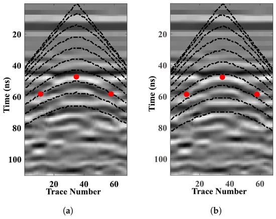
Figure 13.
Traveltime curves of the reference point sources. (a) For ; (b) For .
As shown in Figure 13b, the three characteristic points align parallel to the adjacent travel time curves, confirming that the revised can be regarded as the true relative permittivity of the first layer. Finally, was used to perform time-to-depth conversion on the apex of diffraction hyperbola #1, and this depth (denoted as ) was defined as the lower boundary of the first layer.
Figure 14 presents a scatter plot of the permittivity values estimated at 31 diffraction locations following the workflow described above, with color indicating the permittivity of each point. In addition, we provided a plot of permittivity versus depth (Figure 15). For regions deeper than the bottom interface of the layered model, the permittivity was set to the default value . As shown in Figure 15, the relative permittivity of the lunar regolith increases smoothly with depth, ranging approximately from 2.55 to 6. This trend is consistent with results reported in [35], which were derived from CE-4 LPR data acquired during the first two lunar days.
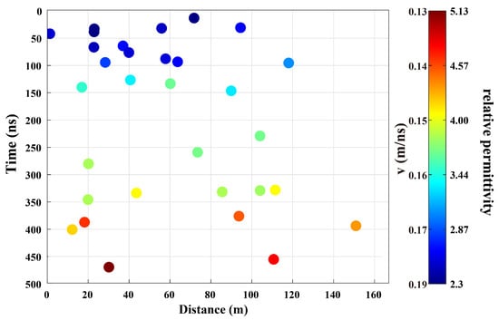
Figure 14.
Relative permittivity scatter plot for 31 diffraction events.
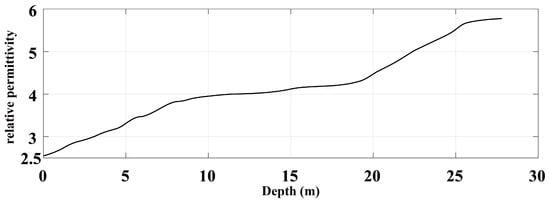
Figure 15.
Variation of the relative permittivity with depth.
Specifically, the relative permittivity varies rapidly within the 0–11 m depth range. This reflects progressive particle fracturing and substantial porosity changes in the shallow regolith, driven by intense space weathering and micrometeorite bombardment. Furthermore, between 11 m and 18 m depth, the rate of permittivity increase moderates, corresponding to a coarse ejecta zone largely unaffected by active surface weathering. In this zone, compaction has stabilized and density growth has slowed. Due to the density-permittivity correlation, this leads to a reduced rate of permittivity increase. Below 18 m, the permittivity rises more sharply, likely due to the proximity of the shallow basalt surface (within about 25 m). Gradual changes in material composition in this region are the direct cause of this accelerated increase.
It should be noted that most HBMs rely on simplified models that assume a horizontally homogeneous subsurface and a point-source reflector. In reality, however, the lunar regolith is often heterogeneous and anisotropic (e.g., tilted stratigraphy and uneven ejecta distribution). Evidently, discrete diffraction objects are insufficient to fully characterize the distribution and variation of the shallow lunar regolith. Therefore, integrating multi-source information, such as geological context and lunar sample data, is essential for reconstructing a reliable shallow regolith structure and for inferring the evolutionary history of the Moon.
5. Discussion
Based on the validated results presented in Section 3 and Section 4, the principal advantages of the proposed method can be summarized as follows: (1) The proposed layer-stripping strategy conducts a sequential, shallow-to-deep velocity scan for diffraction events. Crucially, the velocity analysis of deeper layers is constrained by the results from overlying shallow layers, which is consistent with the inherent depth-dependent gradual variation of subsurface velocity and remarkably enhances the accuracy and reliability of velocity modeling. (2) A “parallelism check” strategy is adopted to convert velocity estimation into a geometric comparison between the characteristic points of diffraction events and simulated travel time curves, featuring an intuitive principle and clear physical meaning. Compared with the traditional direct least-squares optimization method, this strategy eliminates the dependence on initial values, avoids the need to construct complex objective functions, and prevents getting trapped in local optima, thereby improving the stability. (3) The estimated velocity structure can be transformed into a dielectric permittivity model. This enables accurate characterization of subsurface electrical stratification and provides insights into the material composition and physical properties (e.g., water content, porosity) of the medium. (4) The method is particularly suited for common-offset GPR data, primarily because: First, in this acquisition mode, diffraction signals possess focused energy, a higher signal-to-noise ratio, and complete hyperbolic shapes, which enhances the identification and picking of characteristic points; second, time-to-depth conversion with coincident source-receiver geometry eliminates errors associated with offset correction, thereby improving the positioning accuracy of subsurface structures. (5) The proposed method also demonstrates excellent computational efficiency. For example, in the numerical test in Section 3, the velocity analysis for diffraction hyperbola #1 required approximately 5.1 s of CPU time when was fixed at an initial value of 2. For comparison, when was about iteratively swept across 2 to 3.5 with a step size of 0.01, the total CPU time was about 235.9 s, corresponding to an average time of merely 1.56 s per iteration. This efficiency benefits from using the “parfor parallel loop” function in the MATLAB code for the full workflow execution. This computational performance fully confirms that the layer-stripping velocity scanning method maintains satisfactory efficiency while ensuring calculation accuracy (i.e., covering a wide parameter range with fine step size scanning). It therefore provides robust technical support for the rapid processing of large-scale GPR datasets.
Despite the notable merits outlined above, this study has several inherent limitations: (1) This study assumes ideal antenna array operation, neglecting hardware defects such as mutual coupling [36]. In practice, mutual coupling distorts the propagation paths of EM signals and shifts energy distribution, thereby impairing record accuracy. This indirectly compromises the precision of characteristic point extraction, time-to-depth conversion, and velocity estimation. (2) Our layer-stripping strategy assumes that the subsurface has a horizontally layered vertical distribution with uniform intralayer properties. However, the actual subsurface contains non-horizontal geological features such as inclined bedding, lateral abrupt changes in medium properties, and complex fractures. This assumption may introduce discrepancies between the constructed layered model and the true geological structure. (3) The method is to some extent influenced by GPR acquisition parameters: an excessively low center frequency fails to capture signals from small-scale diffractions, while insufficient sampling results in distorted records and loss of waveform details for diffraction waves. Both issues ultimately undermine the accuracy of velocity scanning and the reliability of the constructed model.
Therefore, future research will address the above limitations by constructing an antenna array model through simulation to quantify the relationship between mutual coupling coefficients and signal distortion, incorporating a lateral gradient model into the layer-stripping strategy to optimize model construction, and investigating the correlation between radar acquisition parameters and diffraction-wave identification while adaptively adjusting recognition thresholds or adopting interpolation methods accordingly.
6. Conclusions
HBMs represent a principal and effective approach for estimating subsurface velocity (or dielectric permittivity) distributions from diffraction signals. Conventional approaches often treat velocities at different depths as independent, neglecting the inherent physical continuity between layers, which may lead to inaccuracies in deep velocity estimation. To address this, we proposed a “shallow-control-deep” framework for velocity analysis. It sequentially estimates the velocity of each diffraction event in the radargram from shallow to deep, based on their apex arrival times. Furthermore, velocities derived from shallower layers constrain the scanning of deeper layers, thus improving the estimation accuracy in deep regions. Additionally, within the aforementioned layer-stripping framework, we introduced a “parallelism check” scheme to replace the conventional direct least-squares method. This novel scheme is more intuitive and physically meaningful, and can reduce reliance on complex nonlinear optimization algorithms. The proposed method was first validated on simulated GPR data and then on the LPR field data, aiming to illustrate its workflow and verify its compatibility with monostatic radar configurations. It yielded a permittivity profile of the shallow subsurface (down to 27 m) in the CE-4 landing area, with values ranging approximately from 2.55 to 6. This permittivity profile reveals three distinct zones: (1) From 0 to 11 m, a significant increase suggests abrupt changes in rock grain size within the shallow regolith; (2) From 11 to 18 m, a moderated growth rate indicates a relatively stable layer likely formed by long-term compaction; (3) From 18 to 25 m, a renewed increase is interpreted as a transitional zone between the regolith and the underlying high-permittivity bedrock. Comparison with previously published results from the CE-4 landing site further confirms the accuracy and reliability of the proposed method in reconstructing the electrical structure of the lunar regolith.
Author Contributions
Conceptualization, N.H.; methodology, N.H. and T.L.; software, N.H.; validation, T.L., X.L. and N.L.; formal analysis, N.H. and T.L.; resources, N.H.; data curation, X.L. and N.L.; writing—original draft preparation, N.H. and T.L.; writing—review and editing, X.L. and N.L. All authors have read and agreed to the published version of the manuscript.
Funding
This research was funded by the Jilin Scientific and Technological Development Program (grant number YDZJ202301ZYTS238). This work was also supported by the National Natural Science Foundation of China (Grants No. 42404160, and 42304160).
Institutional Review Board Statement
Not applicable.
Informed Consent Statement
Not applicable.
Data Availability Statement
The data that support the findings of this study are available from the corresponding author, Nan Huai, upon reasonable request.
Acknowledgments
We would like to express our sincere gratitude to the Key Laboratory of Geophysical Exploration Equipment, Ministry of Education (Jilin University) for providing excellent experimental platforms, technical resources, and a favorable research environment for this study. The advanced equipment and professional technical support from the laboratory laid a solid foundation for the analysis of LPR data, as well as the verification of the proposed method. We also appreciate the valuable guidance and assistance from the laboratory staff during the research process.
Conflicts of Interest
The authors declare no conflicts of interest.
Abbreviations
The following abbreviations are used in this manuscript:
| CE-4 | Chang’e-4 |
| EM | Electromagnetic |
| FDTD | Finite-Difference Time-Domain |
| FMM | Fast Marching Method |
| GPR | Ground-Penetrating Radar |
| HBMs | Hyperbola-Based Methods |
| LPR | Lunar Penetrating Radar |
| MAE | Mean Absolute Error |
| PSDs | Parabolic-shaped Diffractions |
References
- Strobach, E.; Harris, B.D.; Dupuis, J.C.; Kepic, A.W. Waveguide properties recovered from shallow diffractions in common offset GPR. J. Geophys. Res. Solid Earth 2013, 118, 39–50. [Google Scholar] [CrossRef]
- Sava, P.C.; Biondi, B.; Etgen, J. Wave-equation migration velocity analysis by focusing diffractions and reflections. In Seismic Diffraction; Society of Exploration Geophysicists: Houston, TX, USA, 2016. [Google Scholar]
- Bauer, A.; Schwarz, B.; Gajewski, D. Utilizing diffractions in wavefront tomography. Geophysics 2017, 82, R65–R73. [Google Scholar] [CrossRef]
- Lin, P.; Zhao, J.; Peng, S.; Cui, X. Diffraction separation by variational mode decomposition. Geophys. Prospect. 2021, 69, 1070–1085. [Google Scholar] [CrossRef]
- Junhong, T.; Jingtao, Z.; Tongjie, S. A neural network-based method for analyzing diffracted wave velocity. Coal Geol. Explor. 2024, 52, 16. [Google Scholar]
- Conyers, L.B. Ground penetrating radar. In Encyclopedia of Imaging Science and Technology; Wiley: Hoboken, NJ, USA, 2002. [Google Scholar]
- Yuan, H.; Montazeri, M.; Looms, M.C.; Nielsen, L. Diffraction imaging of ground-penetrating radar data. Geophysics 2019, 84, H1–H12. [Google Scholar] [CrossRef]
- Lv, W.; Zhang, J. High-resolution permittivity estimation of ground penetrating radar data by migration with isolated hyperbolic diffractions and local focusing analyses. Front. Astron. Space Sci. 2023, 10, 1188232. [Google Scholar] [CrossRef]
- Liu, Y.; Irving, J.; Holliger, K. Weighted diffraction-based migration velocity analysis of common-offset GPR reflection data. IEEE Trans. Geosci. Remote Sens. 2023, 61, 5901509. [Google Scholar] [CrossRef]
- Liu, Y.; Irving, J.; Holliger, K. High-resolution velocity estimation from surface-based common-offset GPR reflection data. Geophys. J. Int. 2022, 230, 131–144. [Google Scholar] [CrossRef]
- Dossi, M.; Forte, E.; Cosciotti, B.; Lauro, S.E.; Mattei, E.; Pettinelli, E.; Pipan, M. Estimation of the subsurface electromagnetic velocity distribution from diffraction hyperbolas by means of a novel automated picking procedure: Theory and application to glaciological ground-penetrating radar data sets. Geophysics 2024, 89, KS53–KS68. [Google Scholar] [CrossRef]
- Shihab, S.; Al-Nuaimy, W. Radius estimation for cylindrical objects detected by ground penetrating radar. Subsurf. Sens. Technol. Appl. 2005, 6, 151–166. [Google Scholar] [CrossRef]
- Giannakis, I.; Zhou, F.; Warren, C.; Giannopoulos, A. On the limitations of hyperbola fitting for estimating the radius of cylindrical targets in nondestructive testing and utility detection. IEEE Geosci. Remote Sens. Lett. 2022, 19, 8029005. [Google Scholar] [CrossRef]
- Ulaby, F.T.; Long, D.; Blackwell, W.J.; Elachi, C. Microwave Radar and Radiometric Remote Sensing; University Michigan Press: Ann Arbor, MI, USA, 2014. [Google Scholar]
- Feng, J.; Su, Y.; Ding, C.; Xing, S.; Dai, S.; Zou, Y. Dielectric properties estimation of the lunar regolith at CE-3 landing site using lunar penetrating radar data. Icarus 2017, 284, 424–430. [Google Scholar] [CrossRef]
- Song, H.; Li, C.; Zhang, J.; Wu, X.; Liu, Y.; Zou, Y. Rock location and property analysis of lunar regolith at Chang’E-4 landing site based on local correlation and semblance analysis. Remote Sens. 2020, 13, 48. [Google Scholar] [CrossRef]
- Dong, Z.; Fang, G.; Zhao, D.; Zhou, B.; Gao, Y.; Ji, Y. Dielectric properties of lunar subsurface materials. Geophys. Res. Lett. 2020, 47, e2020GL089264. [Google Scholar] [CrossRef]
- Fa, W. Bulk density of the lunar regolith at the Chang’E-3 landing site as estimated from lunar penetrating radar. Earth Space Sci. 2020, 7, e2019EA000801. [Google Scholar] [CrossRef]
- Wang, R.; Su, Y.; Ding, C.; Dai, S.; Liu, C.; Zhang, Z.; Hong, T.; Zhang, Q.; Li, C. A novel approach for permittivity estimation of lunar regolith using the lunar penetrating radar onboard Chang’E-4 rover. Remote Sens. 2021, 13, 3679. [Google Scholar] [CrossRef]
- Hamran, S.E.; Paige, D.A.; Amundsen, H.E.; Berger, T.; Brovoll, S.; Carter, L.; Damsgård, L.; Dypvik, H.; Eide, J.; Eide, S.; et al. Radar imager for Mars’ subsurface experiment—RIMFAX. Space Sci. Rev. 2020, 216, 128. [Google Scholar] [CrossRef]
- Casademont, T.; Hamran, S.E.; Amundsen, H.; Eide, S.; Dypvik, H.; Berger, T.; Russell, P. Dielectric permittivity and density of the shallow martian subsurface in Jezero crater. In Proceedings of the 53rd Lunar and Planetary Science Conference, The Woodlands, TX, USA, 7–11 March 2022; Volume 2678, p. 1513. [Google Scholar]
- Liu, R.; Xu, Y.; Chen, R.; Zhao, J.; Xu, X. An improved hyperbolic method and its application to property inversion in Martian Tianwen-1 GPR data. IEEE Trans. Geosci. Remote Sens. 2023, 61, 5104014. [Google Scholar] [CrossRef]
- Zhang, L.; Xu, Y.; Liu, R.; Chen, R.; Bugiolacchi, R.; Gao, R. The dielectric properties of Martian regolith at the Tianwen-1 landing site. Geophys. Res. Lett. 2023, 50, e2022GL102207. [Google Scholar] [CrossRef]
- Ristic, A.V.; Petrovacki, D.; Govedarica, M. A new method to simultaneously estimate the radius of a cylindrical object and the wave propagation velocity from GPR data. Comput. Geosci. 2009, 35, 1620–1630. [Google Scholar] [CrossRef]
- Sethian, J.A. Fast marching methods. SIAM Rev. 1999, 41, 199–235. [Google Scholar] [CrossRef]
- Quell, M.; Diamantopoulos, G.; Hössinger, A.; Weinbub, J. Shared-memory block-based fast marching method for hierarchical meshes. J. Comput. Appl. Math. 2021, 392, 113488. [Google Scholar] [CrossRef]
- Xia, J.; Yang, D.; Tong, P. A high-efficiency parallel fast marching method for large-scale seismic tomography in three-dimensional spherical coordinates. Comput. Geosci. 2025, 196, 105841. [Google Scholar] [CrossRef]
- Irving, J.; Knight, R. Numerical modeling of ground-penetrating radar in 2-D using MATLAB. Comput. Geosci. 2006, 32, 1247–1258. [Google Scholar] [CrossRef]
- Fang, G.Y.; Zhou, B.; Ji, Y.C.; Zhang, Q.Y.; Shen, S.X.; Li, Y.X.; Guan, H.F.; Tang, C.J.; Gao, Y.Z.; Lu, W.; et al. Lunar Penetrating Radar onboard the Chang’e-3 mission. Res. Astron. Astrophys. 2014, 14, 1607. [Google Scholar] [CrossRef]
- Dong, Z.; Fang, G.; Ji, Y.; Gao, Y.; Wu, C.; Zhang, X. Parameters and structure of lunar regolith in Chang’E-3 landing area from lunar penetrating radar (LPR) data. Icarus 2017, 282, 40–46. [Google Scholar] [CrossRef]
- Capineri, L.; Grande, P.; Temple, J. Advanced image-processing technique for real-time interpretation of ground-penetrating radar images. Int. J. Imaging Syst. Technol. 1998, 9, 51–59. [Google Scholar] [CrossRef]
- Kim, S.; Jee Seol, S.; Byun, J.; Oh, S. Extraction of diffractions from seismic data using convolutional U-net and transfer learning. Geophysics 2022, 87, V117–V129. [Google Scholar] [CrossRef]
- Zhang, H.; Li, Y.; Huang, J. Conditional denoising diffusion probabilistic model for seismic diffraction separation and imaging. IEEE Trans. Geosci. Remote Sens. 2024, 62, 5912413. [Google Scholar]
- Casademont, T.M.; Dypvik, H.; Eide, S.; Berger, T.; Hamran, S.E. Martian ground penetrating radar: Towards automated diffraction detection for dielectric permittivity. IEEE Trans. Geosci. Remote Sens. 2024, 62, 4511210. [Google Scholar] [CrossRef]
- Dong, Z.; Feng, X.; Zhou, H.; Liu, C.; Zeng, Z.; Li, J.; Liang, W. Properties analysis of lunar regolith at Chang’E-4 landing site based on 3D velocity spectrum of lunar penetrating radar. Remote Sens. 2020, 12, 629. [Google Scholar] [CrossRef]
- Bazzi, A.; Slock, D.T.; Meilhac, L. On Mutual Coupling for ULAs: Estimating AoAs in the presence of more coupling parameters. In Proceedings of the 2017 IEEE International Conference on Acoustics, Speech and Signal Processing (ICASSP), New Orleans, LA, USA, 5–9 March 2017; IEEE: Piscataway, NJ, USA, 2017; pp. 3361–3365. [Google Scholar]
Disclaimer/Publisher’s Note: The statements, opinions and data contained in all publications are solely those of the individual author(s) and contributor(s) and not of MDPI and/or the editor(s). MDPI and/or the editor(s) disclaim responsibility for any injury to people or property resulting from any ideas, methods, instructions or products referred to in the content. |
© 2026 by the authors. Licensee MDPI, Basel, Switzerland. This article is an open access article distributed under the terms and conditions of the Creative Commons Attribution (CC BY) license.