1. Introduction
The instance selection algorithm [
1], a pivotal preprocessing technique in machine learning, aims to identify representative and high-quality instances from datasets, thereby reducing data volume while preserving or enhancing model performance [
2]. This technique is critical for applications such as dimensionality reduction [
3,
4], outlier detection [
5], knowledge discovery [
6] and incremental learning [
7,
8,
9], where efficient data processing and accurate prediction are paramount. Recent studies on the intersection of Big Data and AI have further emphasized the necessity of integrating robust preprocessing techniques to manage complex, heterogeneous inputs and ensure the interpretability of large-scale systems [
10]. As highlighted in [
10], effective data management and benchmarking strategies are fundamental to optimizing the performance of AI models in data-intensive environments.
Despite significant advancements, traditional instance selection algorithms face inherent limitations that hinder their scalability and precision, particularly in large-scale regression tasks. These methods can be broadly categorized into two classes with distinct drawbacks:
Non-heuristic algorithms (e.g., RegCNN, RegENN [
11]) rely on iterative refinement, where each step depends on the output of previous iterations. This sequential dependency makes parallelization mathematically impossible, severely restricting their scalability.
Heuristic algorithms (e.g., evolutionary-based GA-IS [
12]) support parallel processing but operate at the subset level, leading to coarse-grained selection. Additionally, their reliance on heuristic search increases the risk of converging to local optima, compromising the quality of selected instances.
These limitations highlight a significant gap: the lack of a method that combines the fine-grained precision of individual evaluation with the parallel scalability required for modern datasets.
To bridge this gap, we propose a paradigm shift: evaluating instance quality through cognitive reasoning rather than heuristic search or sequential filtering. Inspired by the logic of Expert Systems [
13] but grounded in vector space theory, we introduce CRDISA (Cognitive Reasoning-Driven Instance Selection Algorithm).
The core innovation of CRDISA is to treat every training instance as an independent “Instance Expert.” Instead of relying on a global model, each expert constructs a difference knowledge base—a tensor representation of its relative position to all other instances in the difference space. This formulation allows each instance to reason about unseen data deterministically. An instance’s quality is then quantified by its reasoning accuracy: if an instance can accurately infer the targets of validation samples using its local difference knowledge, it is deemed a high-quality prototype.
CRDISA addresses the limitations of prior works through three key contributions:
- 1.
Theoretical Formalization of Instance Quality: We move beyond metaphorical descriptions by mathematically defining “cognition” as a first-order difference field. This allows for a rigorous, fine-grained evaluation of individual instances, avoiding the randomness of heuristic methods.
- 2.
Adaptive Regression Evaluation: To handle continuous targets, we propose a soft partitioning strategy that establishes dynamic error boundaries based on local data variance, coupled with a bidirectional voting mechanism to filter noise.
- 3.
Distributed Architecture for Scalability: The construction of individual knowledge bases creates a computational complexity of . To make this theoretically rigorous approach practically viable, we implement CRDISA on Apache Spark. By leveraging Spark’s in-memory computing and an optimized broadcast mechanism, we eliminate sequential bottlenecks and minimize shuffle operations, parallelizing the quadratic workload to achieve linear scalability in wall-clock time with respect to computing resources.
The remainder of this paper is structured as follows:
Section 2 reviews related work on instance selection and distributed computing framework.
Section 3 details the theoretical framework and mathematical definitions of CRDISA.
Section 4 describes the distributed implementation on Apache Spark.
Section 5 presents the experimental analysis, and
Section 6 concludes the study.
2. Related Work
2.1. Instance Selection Algorithm
In classification tasks, instance selection algorithms are mainly categorized into Wrapper and Filter methods [
14]. The Wrapper methods remove redundant and noisy instances based on a specific classifier, such as the Condensed Nearest Neighbor (CNN), the Edited Nearest Neighbor (ENN), the DROP1-5 family of algorithm [
15], the Stochastic Perturbation Instance Selection (SpIS) [
16], SpFixedIS [
17] and evolutionary based instance selection methods [
12,
18,
19], etc. In contrast, The Filter methods adopt a function-based selection strategy and usually employ clustering techniques to select boundary or central instances within each class, such as the Pattern by Ordered Projections (POP) [
20] and the Pair Opposite Class-Nearest Neighbor (POC-NN) [
21], etc. A comprehensive review of instance selection algorithms for classification tasks is provided in the literature [
22], including their classification criteria, advantages and disadvantages.
Regression tasks, characterized by continuous output spaces, pose unique challenges for instance selection, as instance quality cannot be easily determined by class boundaries. Existing methods primarily fall into two categories [
23]:
(1) Evolutionary-based methods: These extend multi-objective optimization to balance dataset compression and prediction error. Antonelli et al. [
24] proposed a coevolutionary framework for fuzzy rule-based systems, while Kordos et al. [
25] optimized subsets for minimal error or size. García-Pedrajas et al. [
26] mitigated local optima by combining independent sub-population evolution with cooperative evaluation, while literature [
27] employed clustering (e.g., k-means, fuzzy C-means) for population partitioning. Although such methods support limited parallelization, they inherently rely on subset-level search, resulting in coarse granularity and vulnerability to local optima.
(2) Nearest neighbor-based methods: Arnaiz-González et al. [
28] adapted classification-oriented methods to regression by discretization. Song et al. [
29] removed outlier instances and indistinctive instances to decrease the size of training set for KNN regression. Kordos et al. [
11] obtained the classic RegCNN and RegENN by extending CNN and ENN algorithms. Guillen et al. [
30] used mutual information to evaluate the importance of input vectors in time series, effectively identifying outliers and noise but incurring high computational costs for large datasets. The DROP3-RE algorithm [
31] selects instances based on error accumulation.
Notably, both categories struggle to reconcile fine-grained individual evaluation with efficient parallelization. Evolutionary methods prioritize parallelizability but sacrifice granularity, while nearest neighbor methods focus on individual instances but rely on sequential iterations. This gap motivates our approach of endowing individual instances with cognitive reasoning capabilities to enable parallelizable, instance-level quality assessment.
2.2. Distributed Computing Framework: Apache Spark
Apache Spark is an open-source distributed computing framework designed for large-scale data processing, supporting batch processing, real-time streaming, machine learning, and graph computations [
32,
33,
34,
35]. Its Resilient Distributed Dataset (RDD) [
36] and in-memory computing enable efficient parallel processing of large-scale data, with core operations supporting distributed transformation and aggregation.
The following introduces the key operations used in this work:
map(func): Perform the user-defined converting function on each element in the and return a new with the transformed elements.
reduce(func): This performs the aggregation on each element of the , and func is used to define the way of aggregation.
mapPartitions(func): It is similar to map(func), but operates on partitions instead of individual elements, which is generally more efficient.
zipWithIndex(): Add an index to each element of the in order and return key-value pairs. For example, for a dataset .
randomSplit(weights, seed): Split an into two new based on the specified weights and randomness controlled by seed.
collect(): Gather elements on different computing nodes into the driver node as a local variable.
cache(): Store the elements of the into memory for faster future access.
2.3. Theoretical Comparison of Instance Selection Frameworks
While existing algorithms and CRDISA share the goal of data reduction, they differ fundamentally in their theoretical constraints and operational mechanisms.
Table 1 summarizes the distinctions between traditional instance-centric methods (e.g., RegCNN [
11]) and our Cognitive Reasoning-Driven approach.
The most critical difference lies in the Operational Paradigm. Traditional methods employ a “Passive Filtering” approach, where instances are evaluated by a global heuristic (e.g., class boundaries or noise levels). In contrast, CRDISA introduces an “Active Reasoning” paradigm. Each instance is modeled as an autonomous agent that actively predicts the targets of unseen validation data using its local difference knowledge. Consequently, the selection is determined by the instance’s capability to generalize, rather than its static geometric position.
3. The CRDISA Theoretical Framework
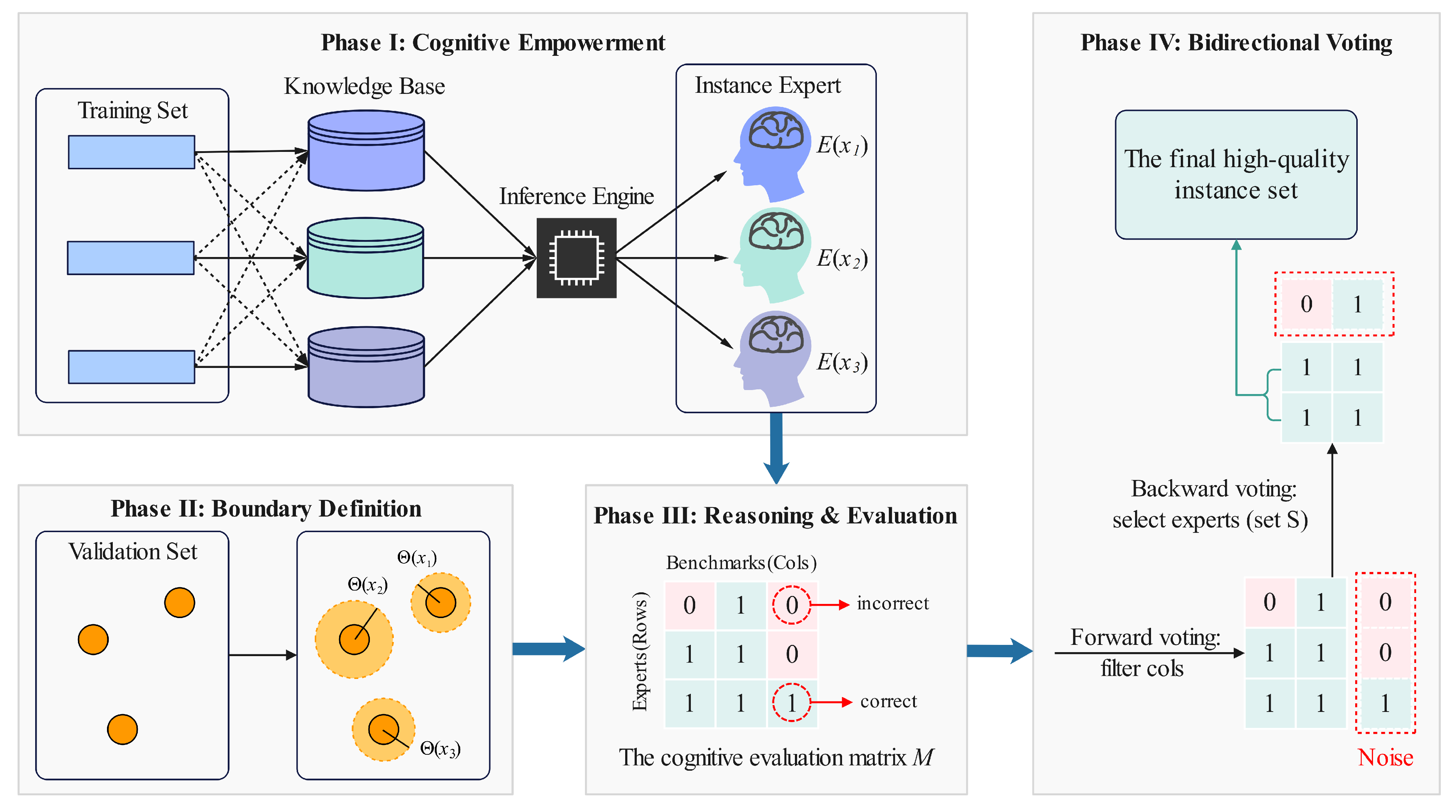
CRDISA establishes a theoretical framework where individual instances are endowed with the cognitive capability to independently reason about global data patterns, thereby transforming into “Instance Experts” capable of reasoning about unseen data, with their quality determined by reasoning accuracy. The theoretical framework of CRDISA is illustrated in
Figure 1.
The framework operates through four interconnected stages: (1) Cognitive Empowerment, where instances construct their own difference knowledge bases and inference engines, transforming into “Instance Experts”; (2) Boundary Definition, calculating adaptive soft boundaries for validation data; (3) Reasoning and Evaluation, where instances infer targets and are scored based on accuracy; and (4) Bidirectional Voting, filtering noise to select the final high-quality instance set.
In this section, we provide the formal definitions of the cognitive reasoning mechanism, the soft partitioning strategy for regression, and the bidirectional voting mechanism. Finally, we present a theoretical analysis of the algorithm’s computational complexity.
3.1. Formal Definitions of Cognitive Reasoning
To mathematically ground the concept of “Cognitive Reasoning” and avoid metaphorical ambiguity, we formalize it as an instance-centric similarity reasoning process within a first-order difference field. In this framework, we use the term “Cognition” to characterize the system’s architectural shift from passive geometric filtering to active, agent-based self-evaluation. Specifically:
“Cognition” refers to the instance’s autonomous capability to construct a subjective worldview (mathematically, the Difference Knowledge Base defined below).
“Reasoning” refers to the active inference process where the instance validates its own utility through a hypothesis-verification mechanism.
Definition 1 (First-Order Difference/Atomic Cognition)
. The fundamental unit of cognition in our framework is the relative difference between two instances. For any two instances and in the dataset, the First-Order Difference is defined as a vector pair representing the positional shift in both feature and target spaces:where and . This difference vector quantifies how instance perceives instance . Definition 2 (Difference Knowledge Base)
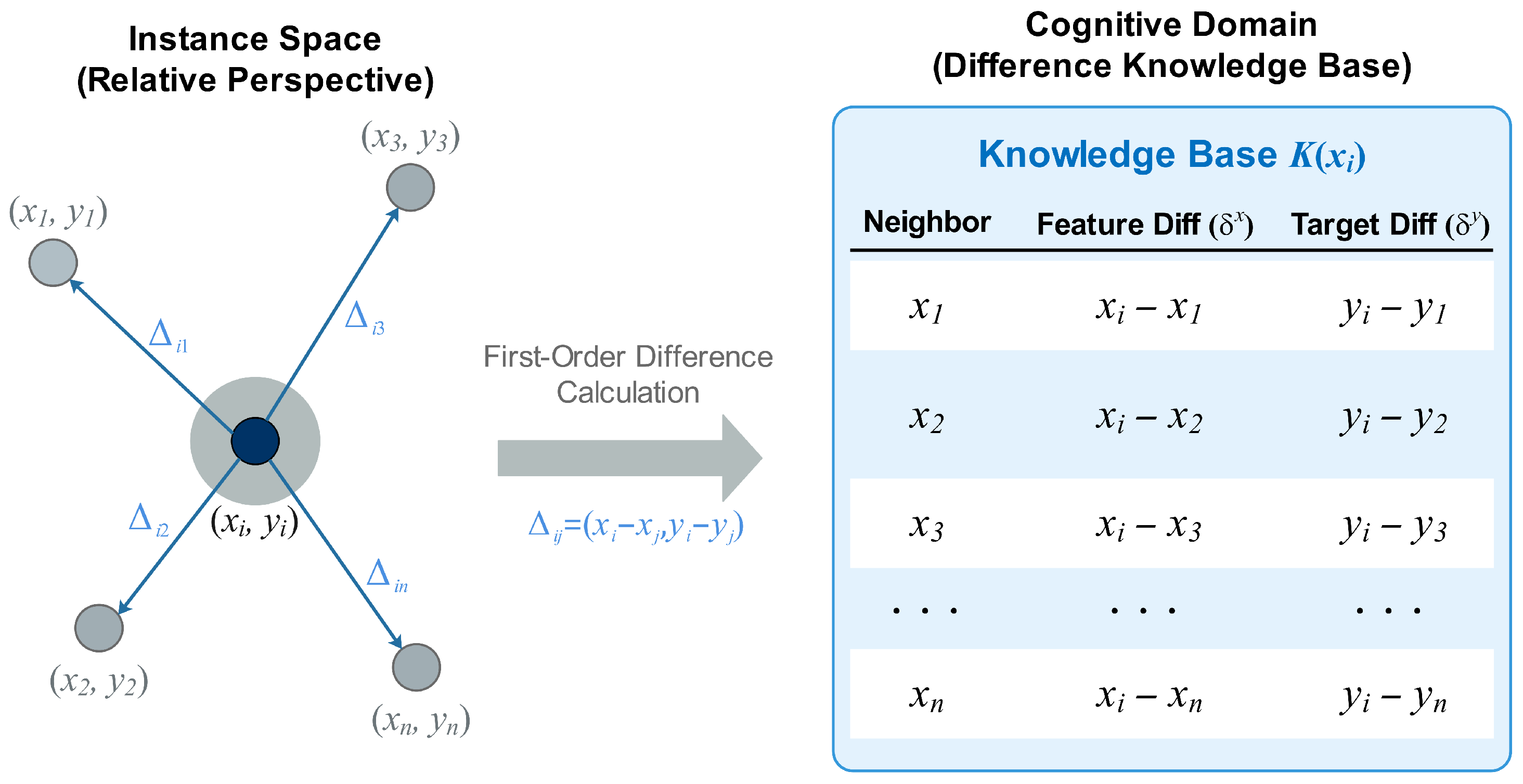
. By aggregating the atomic cognitions of an instance relative to the entire dataset, we construct its cognitive domain. The Difference Knowledge Base is defined as a tensor containing the set of all first-order differences centered at : This structure ensures that the “cognition” is unique (derived from
’s specific perspective), consistent (covers the whole dataset), and comprehensive. The construction process of these difference knowledge bases is visualized in
Figure 2. As shown, each instance performs difference operations with all peers to populate its private knowledge base.
Definition 3 (Instance Expert)
. Let be the training dataset. With the knowledge base established, we formally define the instance expert as an autonomous agent capable of reasoning. An instance expert is a tuple:where and represent the original feature vector and the target value of the instance respectively, is the unique difference knowledge base (its memory), and is the unified inference engine, standardized as a k-Nearest Neighbor logic operating within the difference space. Definition 4 (Instance Reasoning Process)
. The reasoning process is a mapping function executed by the inference engine of expert on an unseen validation instance . The expert predicts the target by retrieving patterns from : Here, represents the indices of the k difference vectors in whose feature differences minimize the Euclidean distance to the query difference . This formulation allows the expert to infer the result based on how similar historical differences map to target shifts.
3.2. Evaluation of Reasoning Results Based on Soft Partitioning Strategy
In regression tasks, defining a rigid global threshold for “accurate reasoning” is ill-posed due to the continuous nature of the output. To address this, we propose a soft partitioning strategy that evaluates reasoning results by establishing adaptive boundaries based on local data uncertainty, and subsequently aggregates these results into a global evaluation matrix.
Step 1: Adaptive Soft Boundary Calculation. For a validation instance
(where
), the acceptable error margin is determined by the volatility of its local neighborhood. We define the soft boundary
as:
where
denotes the set of target values of the
k-nearest neighbors of
.
represents the standard deviation, which quantifies the variability of local data distributions.
is a sensitivity hyperparameter adjusting the strictness of the boundary. While statistically associated with confidence intervals (e.g.,
covers 95% density under Gaussian assumptions), our empirical sensitivity analysis (detailed in
Section 5.2.4) identifies the robust operating range as
.
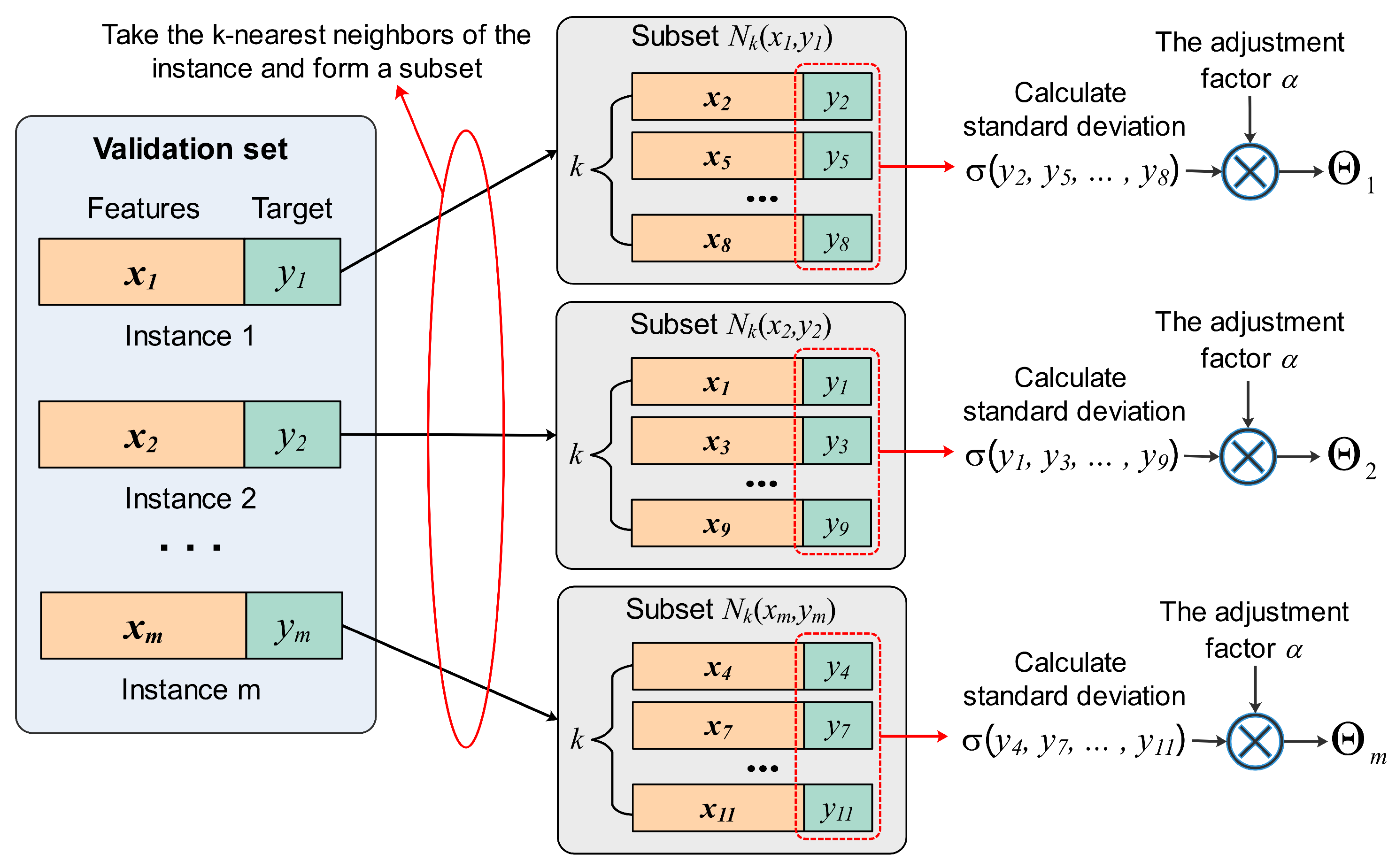
Figure 3 demonstrates how these boundaries are dynamically calculated based on local density and variance.
The definition of the adaptive boundary is grounded in both statistical uncertainty estimation and local function approximation theory.
(1) Adaptation to Local Landscape: The standard deviation reflects the “speed of changes” of the target variable within the local neighborhood. A high indicates a region with steep gradients or high volatility, where prediction is inherently more difficult. By making the threshold proportional to , the algorithm dynamically expands its tolerance in these complex regions to avoid incorrectly rejecting valid instances, while tightening the boundary in smooth regions to maintain precision.
(2) Handling Heteroscedasticity: Regression datasets frequently exhibit heteroscedasticity, where noise variance changes across the feature space. Our formulation effectively constructs a Local Confidence Interval. According to Chebyshev’s Inequality, the probability of a valid instance deviating from its local mean by more than is bounded. Thus, serves as a statistical scaling factor that adjusts the strictness of the boundary relative to the intrinsic local uncertainty.
Step 2: Construction of Cognitive Evaluation Matrix. Based on the soft boundaries, we evaluate the reasoning performance of all
n experts on all
m validation instances. We define the cognitive evaluation matrix as a binary matrix
:
Here,
indicates that Expert
successfully reasoned about validation instance
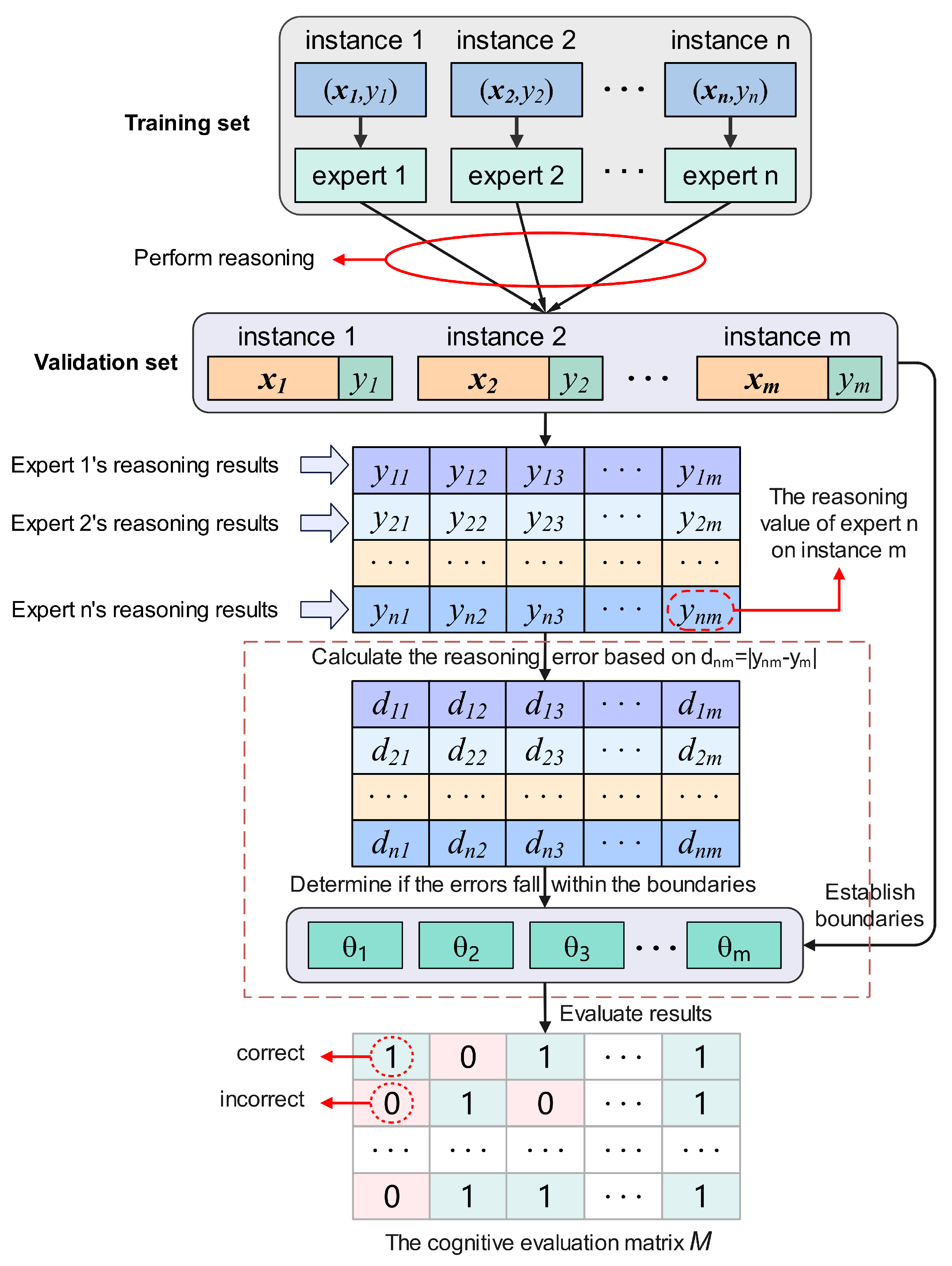
within the acceptable error margin. This matrix consolidates the dispersed reasoning results into a structured format for global analysis. The process of generating this matrix is shown in
Figure 4.
3.3. Bidirectional Voting Mechanism
To identify high-quality instances robustly, we employ a voting mechanism that operates directly on the cognitive evaluation matrix M. This mechanism filters noise through a two-stage consensus protocol. The selection process involves filtering both the validation benchmarks (columns of M) and the instance experts (rows of M):
(1) Forward Voting (Reliability Check): We first identify “Reliable Benchmarks” in the validation set. A validation instance
is deemed reliable if it achieves consensus among the majority of experts. The set of reliable benchmark indices
is defined as:
(2) Backward Voting (Expert Selection): The quality of a training instance (expert)
is then assessed based solely on its performance on the reliable benchmarks. The final high-quality subset
S is selected as:
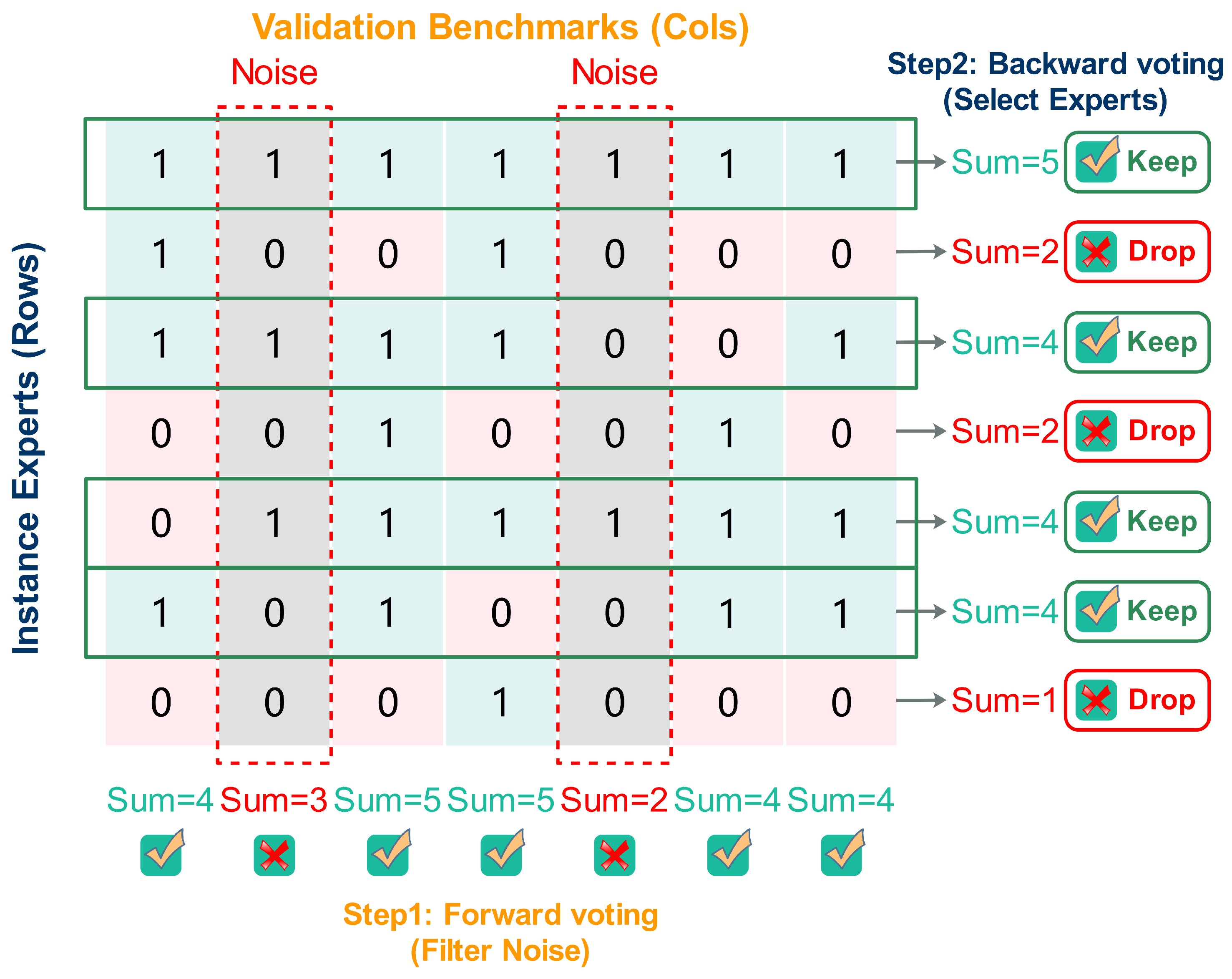
Figure 5 illustrates this data flow. The strict majority thresholds defined in Equations (
7) and (
8) are fundamentally grounded in the principles of Ensemble Learning and Condorcet’s Jury Theorem, ensuring robustness through three key mechanisms:
(1) Robustness to Noise: In regression tasks, expert errors often follow skewed distributions. Aligning with Condorcet’s Jury Theorem, provided that individual experts perform better than random guessing, the strict majority threshold (>
2) statistically maximizes the probability of a correct consensus. This acts as a robust aggregation function (similar to a median filter), ensuring the selection is driven by the consistent signal shared among experts rather than being swayed by the bias of noisy experts [
23].
(2) Decorrelation Strategy: The validity of the jury theorem relies on expert independence. CRDISA fosters this through geometric diversity: each Instance Expert reasons using a unique Difference Knowledge Base derived from its specific relative position in the vector field. This structural diversity naturally de-correlates prediction errors, fulfilling the independence assumption required for effective voting.
(3) Handling Edge Cases: The mechanism addresses issues like small or noisy validation sets via a Balanced Split Strategy (Algorithm 2), ensuring the validation set scales linearly with the dataset (). Furthermore, the Forward Voting acts as a pre-filter to discard non-consensual validation instances.
Consequently, this protocol ensures that the final selection is grounded in consistent performance on objective, high-confidence benchmarks, thereby minimizing the risk of overfitting to noisy validation data.
3.4. Computational Complexity and Scalability Analysis
A critical aspect of CRDISA is its computational complexity. Here we analyze the theoretical bounds and justify the distributed implementation.
Theorem 1 (Construction Complexity). Constructing the Difference Knowledge Base for all n instances requires computing pairwise differences between the instance itself and the entire dataset.
Time Complexity: , where d is the feature dimension.
Space Complexity: Storing the full difference tensor implies .
Theorem 2 (Reasoning Complexity). During the cross-experimentation phase, each of the n experts infers the targets for m validation instances (where in cross-validation).
Scalability Justification: The quadratic complexity
presents a theoretical bottleneck for single-node execution. CRDISA addresses this via the distributed architecture described in
Section 4:
Space Complexity and Memory Distribution: The global difference tensor is never fully materialized on a single node. Through the uniform partition strategy, each executor holds only a subset of experts, approximately (where P is the number of partitions). Consequently, the local memory requirement for each executor is reduced to . This relationship indicates that even as the total dataset size N increases, the memory footprint per node remains stable and bounded, provided that the number of partitions P is scaled proportionally.
Communication Optimization: By broadcasting the raw dataset (size ) to executors instead of shuffling the difference tensors, we reduce the network transmission cost significantly.
Parallel Execution: While the total algorithmic work remains , the wall-clock time T is reduced by the cluster size P: . This linear speedup allows the algorithm to handle larger-scale regression tasks by scaling horizontal resources, as validated in the experimental section.
4. Implementation of CRDISA on Apache Spark
While the theoretical framework of CRDISA ensures fine-grained instance selection, the construction of difference knowledge bases introduces a computational complexity of . To make this rigorous approach practically feasible for large-scale datasets, we implement CRDISA on Apache Spark, a distributed computing framework optimized for in-memory processing.
The implementation leverages Spark’s Resilient Distributed Datasets (RDDs) to parallelize the creation of instance experts and the broadcast mechanism to minimize network overhead. The overall implementation workflow consists of a preprocessing module for data partitioning and load balancing, and a distributed cross-experimentation module for executing the cognitive reasoning logic. The high-level algorithmic framework is described in Algorithm 1.
| Algorithm 1 Cognitive Reasoning-Driven Instance Selection Algorithm (CRDISA) |
- Require:
Original dataset , Number of partitions P, Nearest neighbors k, Sensitivity hyperparameter - Ensure:
Final set of high-quality instances - 1:
// Phase 1: Distributed Preprocessing - 2:
{See Algorithm 2} - 3:
- 4:
// Phase 2: Cross-Experimentation (2 Iterations) - 5:
for do - 6:
if then - 7:
Swap() - 8:
end if - 9:
// Step 1: Construct Instance Experts via Broadcast - 10:
{See Algorithm 3} - 11:
// Step 2: Calculate Soft Boundaries for Validation Set - 12:
- 13:
- 14:
// Step 3: Generate Cognitive Evaluation Matrix M - 15:
{See Algorithm 4} - 16:
// Step 4: Select Instances via Bidirectional Consensus - 17:
{See Algorithm 5} - 18:
- 19:
end for - 20:
return
|
4.1. Preprocessing Module
The preprocessing module prepares the raw data for distributed computation by ensuring logical traceability and balanced workloads across the cluster.
Data Splitting and Indexing: The raw dataset is loaded and randomly partitioned into two subsets of approximately equal size using randomSplit([0.5, 0.5]). Crucially, since instances will be shuffled across nodes, we assign a unique global identifier to each instance using zipWithIndex. This ID allows us to trace the “Instance Expert” back to the original data point throughout the distributed reasoning process.
Uniform Partitioning for Load Balancing: To prevent data skew—a common bottleneck where one node processes significantly more data than others—we implement a uniform partitioning strategy (Algorithm 2). The instances are distributed across
P partitions based on their indices:
where
is the instance index and
N is the total count. This ensures that each executor processes an equal number of experts, maximizing parallel efficiency.
| Algorithm 2 Distributed Preprocessing |
- Require:
Dataset , Number of Partitions P - Ensure:
Balanced RDDs - 1:
Split into using randomSplit([0.5, 0.5]) - 2:
for each in do - 3:
- 4:
- 5:
Function : - 6:
return - 7:
- 8:
- 9:
end for - 10:
return
|
- 3.
Caching: The partitioned are cached in memory using cache() to eliminate redundant disk I/O during the iterative cross-experimentation phases.
4.2. Distributed Cross-Experimentation Module
The core logic of CRDISA is executed in this module. It utilizes the broadcast mechanism to overcome the communication bottlenecks associated with the complexity. Specifically, the and obtained from the Preprocessing Module are alternately employed as the internal training set and internal validation set across two iterations. This dual-iteration strategy ensures that all instances are evaluated both as “instance experts” and as validation targets, thereby enhancing the robustness of the selection process.
4.2.1. Parallel Construction of Instance Experts via Broadcast
Constructing the Difference Knowledge Base for every instance requires computing differences against the entire dataset. A naive distributed implementation would require shuffling massive amounts of difference vectors between nodes, leading to network congestion.
We optimize this using Spark’s Broadcast Variable. Instead of transmitting the generated differences (size ), we broadcast the compact raw dataset (size ) to all executors:
The complete training set is collected to the driver and broadcast as a read-only variable .
Each executor constructs the knowledge bases and initializes the Inference Engines strictly within local memory using mapPartitions (Algorithm 3).
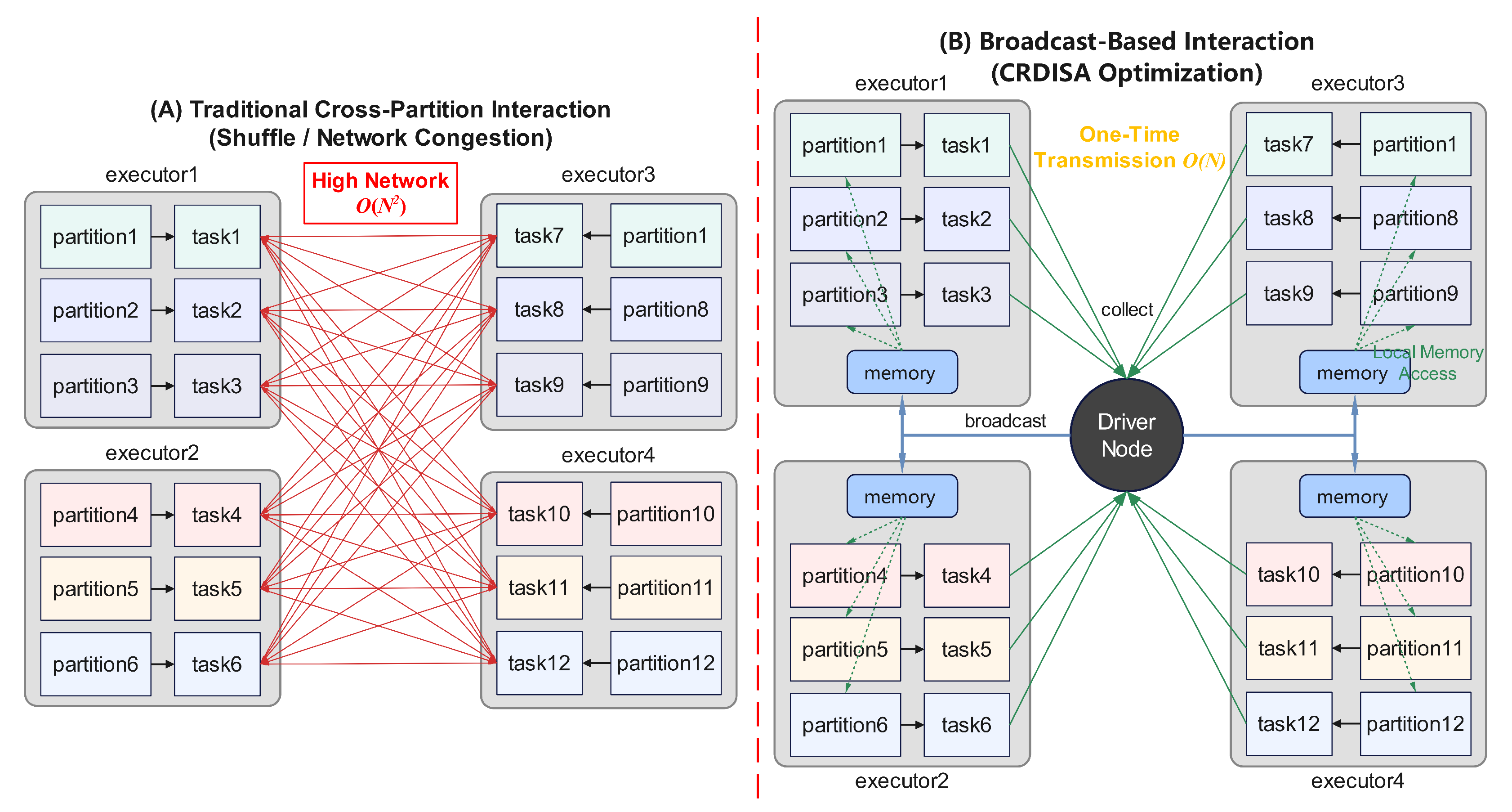
As illustrated in
Figure 6, this strategy transforms an
network transmission problem into an
one, significantly reducing communication overhead.
Figure 6.
Comparison between traditional cross-partition instance interaction and the broadcast-based optimization. Broadcasting the raw dataset reduces network complexity from quadratic to linear.
Figure 6.
Comparison between traditional cross-partition instance interaction and the broadcast-based optimization. Broadcasting the raw dataset reduces network complexity from quadratic to linear.
| Algorithm 3 Parallel Construction of Instance Experts |
- Require:
Iterator of Local Instances (), Broadcast TrainingSet () - Ensure:
Iterator of Instance Experts - 1:
- 2:
{Retrieve broadcasted raw data} - 3:
for each instance in do - 4:
- 5:
for each in do - 6:
{Calculate First-Order Difference} - 7:
- 8:
end for - 9:
{Init Inference Engine} - 10:
{Definition 3} - 11:
- 12:
end for - 13:
return
|
4.2.2. Distributed Soft Boundary Calculation
Before reasoning, the system also leverages the broadcast mechanism to calculate the soft boundaries for the validation set in parallel.
The validation set is broadcast to all nodes.
Executors compute the local neighborhood variance for each validation instance
to determine
(as defined in
Section 3.2).
The resulting boundaries are collected and broadcast back as a map: . This ensures that every expert, regardless of its location in the cluster, uses the same standard to evaluate a specific validation instance.
4.2.3. Evaluate Reasoning Results
With the experts prepared and boundaries defined, the system generates the evaluation matrix
M (Algorithm 4).
| Algorithm 4 Distributed Reasoning and Evaluation (Generating Matrix M) |
- Require:
Iterator of Experts , Broadcast ValidationSet (), Broadcast Thresholds () - Ensure:
Iterator of (Expert_ID, Binary_Vector) - 1:
- 2:
- 3:
- 4:
for each Expert in do - 5:
- 6:
for to do - 7:
- 8:
{Definition 4} - 9:
- 10:
if then - 11:
- 12:
else - 13:
- 14:
end if - 15:
end for - 16:
- 17:
end for - 18:
return
|
Each partition of the (containing local experts ) iterates through the broadcasted validation set. The inference engine predicts targets .
The predictions are immediately compared against the broadcast . This generates a partial row of the matrix M for each expert.
The results are stored as , where each element is a key-value pair (, ). This effectively represents the distributed storage of matrix M.
4.2.4. Distributed Bidirectional Voting
The final step implements the Bidirectional Consensus Protocol using distributed aggregation operations. The implementation logic is shown in Algorithm 5.
Forward Voting (Column-wise Aggregation): We compute the quality of validation instances by summing the votes in column-wise. This is achieved efficiently using with vector addition. Indices of validation instances that pass the consensus threshold are identified as and broadcast to the cluster.
Backward Voting (Row-wise Filtering): We filter the using mapPartitions. For each expert (row), we sum the votes only at the indices specified in . Experts exceeding the acceptance threshold constitute the final selected set S.
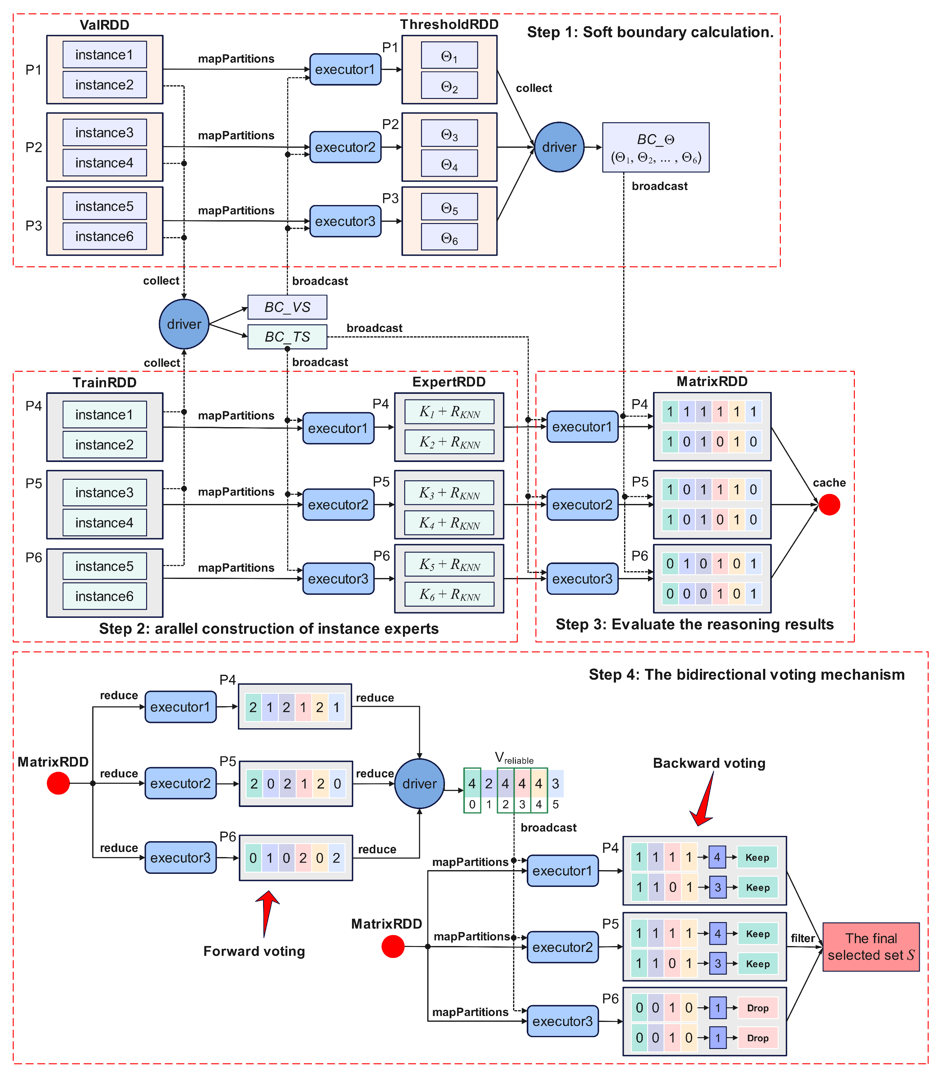
By combining uniform partitioning with broadcast-based data sharing, CRDISA effectively mitigates the computational intensity of the cognitive reasoning framework, achieving the linear scalability required for large-scale regression tasks. The flow of this phase is visualized in
Figure 7.
Figure 7.
The implementation flow of CRDISA’s cross-experimentation module on Spark. It details the data flow from matrix generation to forward voting (reduce) and backward voting (filter).
Figure 7.
The implementation flow of CRDISA’s cross-experimentation module on Spark. It details the data flow from matrix generation to forward voting (reduce) and backward voting (filter).
| Algorithm 5 Bidirectional Voting |
- Require:
MatrixRDD (Rows of Matrix M) - Ensure:
Selected Instance IDs S - 1:
// Step 1: Forward Voting (Column-wise) - 2:
- 3:
- 4:
- 5:
for to do - 6:
if then - 7:
{Identify reliable benchmark indices} - 8:
end if - 9:
end for - 10:
- 11:
// Step 2: Backward Voting (Row-wise) - 12:
Function: - 13:
- 14:
- 15:
- 16:
for each in do - 17:
- 18:
if - 19:
- 20:
end if - 21:
end for - 22:
return - 23:
- 23:
return S
|
5. Experimental Analysis
To validate the theoretical soundness and distributed efficiency of CRDISA, we conducted extensive experiments on 22 regression datasets. The evaluation focuses on three key dimensions: (1) the effectiveness of the cognitive reasoning framework in preserving predictive accuracy; (2) the efficiency of the Bidirectional voting in data compression; and (3) the scalability of the Spark implementation in handling the computational complexity.
5.1. Experimental Setup
Datasets and Environment: We selected 22 regression datasets from the KEEL repository [
37], ranging from small-scale real-world problems to larger synthetic datasets (up to 40,768 instances), as detailed in
Table 2. While the instance counts are moderate by industrial standards, they are sufficient to stress-test the
complexity of the knowledge base construction, serving as effective proxies for analyzing distributed performance. All features were normalized to
to ensure isotropic reasoning in the difference space.
The experiments were executed on a High-Performance Computing cluster (Central South University) with Intel Xeon Gold 6248R CPUs (3 GHz), 192 GB RAM, and 48 cores, using Apache Spark 3.1.2, Hadoop 3.3.0, and Python 3.8.18.
Baselines: Given the scarcity of distributed instance selection algorithms for regression, CRDISA is benchmarked against four representative single-machine methods. To ensure a fair comparison, we avoided arbitrary tuning; instead, the hyperparameters for all baseline methods were fixed to the optimal values recommended in their respective original studies, ensuring they represent standard best practices:
While the selection phase utilized the method-specific parameters above, the final evaluation employed a uniform KNN regressor (
) for all methods. Grounded in literature [
29] citing
as statistically robust, this protocol eliminates confounding variables, ensuring that performance metrics reflect solely the quality of the selected subsets.
Evaluation Metrics: Performance evaluation is conducted using five metrics covering predictive accuracy, compression efficiency, and distributed parallel performance, with detailed definitions and evaluation criteria as follows:
Coefficient of Determination (): Measures the predictive power of the selected experts, where a higher value indicates better performance.
Retention Rate (
m): Quantifies the compression efficiency of instance selection, defined as:
where
S denotes the set of selected instances and
represents the original training set. A lower value of
m indicates better compression performance.
Weighted Indicator (
): A composite metric balancing accuracy and compression efficiency, defined as:
A lower value signifies a higher (better accuracy) and a lower m (better compression), indicating overall superior performance.
Speedup, Sizeup, and Scaleup: Standard metrics to evaluate distributed parallel performance.
Average Rank (AR): Represents the mean rank of the method across all datasets, where a lower value indicates better overall performance.
We employed a 10-fold cross-validation protocol to minimize randomness. In this protocol, the dataset is divided into ten folds; for each round, nine folds serve as the input for the instance selection algorithm, while the remaining fold is used strictly for testing. Crucially, to prevent data leakage, the instance selection process is confined exclusively to the nine input folds (90% of the dataset). The test set remains completely isolated during the selection phase and is used solely for the final evaluation of the trained model. Consequently, the reported and retention rates represent the average performance across these ten independent rounds.
The statistical significance of differences between CRDISA and the baselines was assessed using the Wilcoxon signed-rank test. The null hypothesis posits that no significant differences exist between CRDISA and the competing methods, with the significance level set at
. To strictly control the Family-Wise Error Rate (FWER) in multiple comparisons, we applied the Holm–Bonferroni sequential correction [
38]. Under this stepwise procedure, the null hypotheses are ordered by their
p-values (
) and tested sequentially against dynamic thresholds
(where
m is the total number of independent tests, and
i denotes the rank of the null hypothesis in the sorted
p-value list). A difference is considered statistically significant only if the corresponding null hypothesis is rejected in this sequence.
5.2. Performance Evaluation on Effectiveness
5.2.1. Predictive Accuracy ()
Table 3 presents the detailed
comparison across all datasets. CRDISA achieved an average
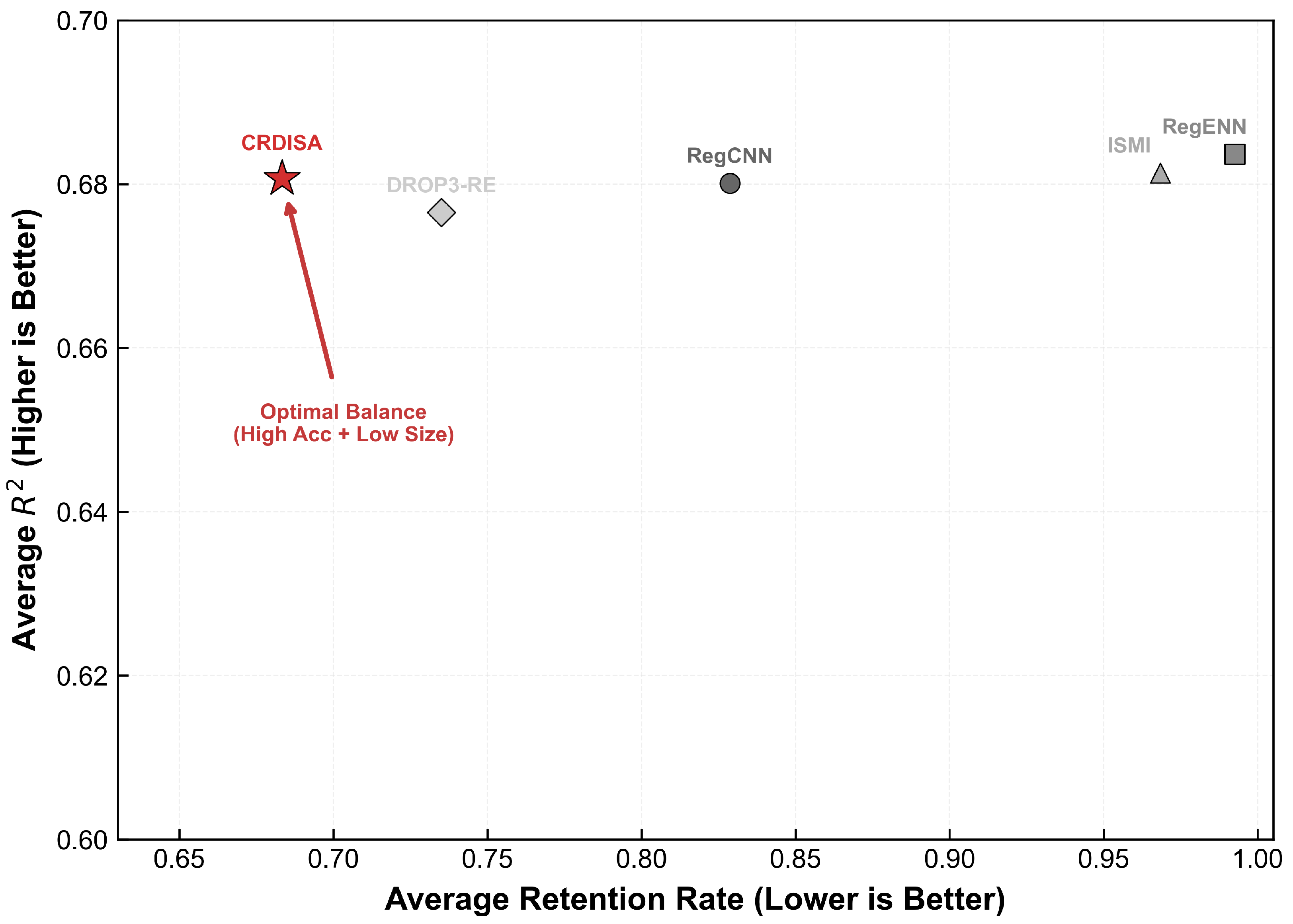
of 0.681. As visualized on the vertical axis of the Trade-off Plot (Figure 9), CRDISA maintains predictive accuracy statistically comparable to RegCNN (0.680,
), ISMI (0.681,
), and DROP3-RE (0.677,
). Regarding RegENN (0.684), while the raw
p-value (
) appeared marginal, the application of the Holm–Bonferroni correction confirms the lack of significance. Specifically, this lowest p-value failed to meet the initial rejection threshold of
(
). Consequently, the null hypothesis holds, statistically confirming that there is no significant difference in predictive performance between CRDISA and any of the state-of-the-art baselines.
The robustness of CRDISA can be attributed to the instance expert model. Unlike heuristic methods that optimize a global objective (often getting trapped in local optima), CRDISA’s soft partitioning strategy (
Section 3.2) adapts the error tolerance
to the local variance of each validation instance. This ensures that selected instances are not just “geometrically central” but “cognitively competent” in high-uncertainty regions. For example, on complex datasets like Airfoil (AIR), CRDISA (0.276) significantly outperforms ISMI (0.249), proving that cognitive reasoning captures non-linear manifolds better than mutual information alone.
5.2.2. Compression Efficiency (Retention Rate m)
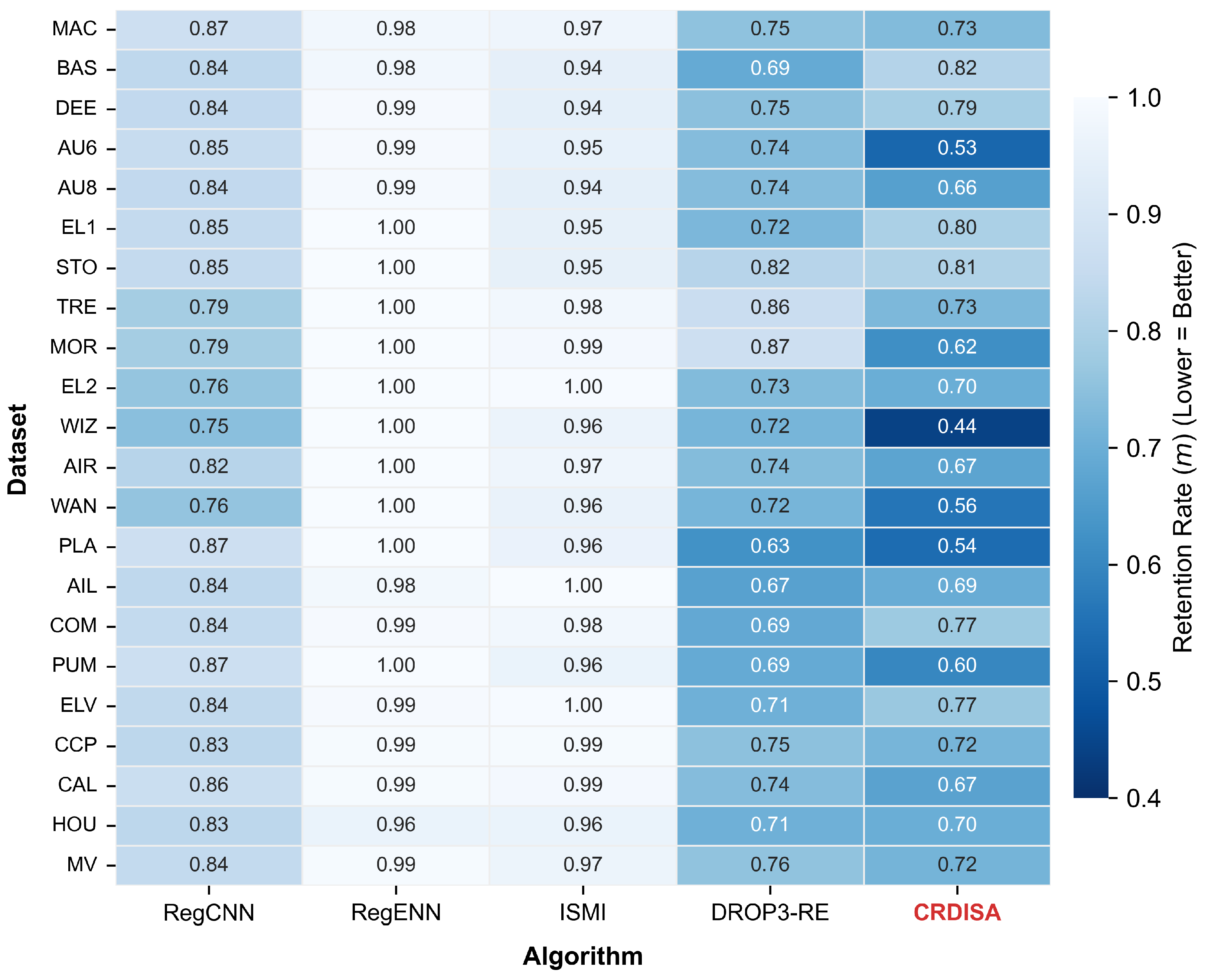
The compression efficiency of CRDISA is evaluated both quantitatively in
Table 4 and visually in the retention rate heatmap (
Figure 8). As illustrated in
Figure 8, the CRDISA column is consistently distinguished by distinct coloring across most datasets, which intuitively reflects its lower retention rates compared to competing algorithms. Quantitatively, CRDISA achieves the lowest average retention rate of 0.683 (31.7% compression), significantly outperforming RegCNN (0.829) and the highly conservative RegENN (0.993). Notably, this advantage is pronounced even on large-scale datasets such as Mv and California, where CRDISA effectively reduces data redundancy while preserving the integrity of critical data patterns required for reliable instance selection.
This high compression rate validates the efficacy of the bidirectional consensus protocol. The forward voting step aggressively filters out noisy validation benchmarks, preventing them from “saving” redundant training instances. The backward voting then ensures that only experts with broad applicability (high consensus) are retained. In contrast, iterative methods like DROP3-RE () often retain redundant instances due to the “error shielding” effect in sequential processing. Wilcoxon signed-rank tests with Holm–Bonferroni correction confirm CRDISA’s statistically significant superiority in compression against all baselines. Specifically, regarding the marginal p-value of 0.046 (against DROP3-RE), the difference remains statistically significant because it appears at the final step of the Holm–Bonferroni sequence, where the rejection threshold relaxes to the full . This confirms that all comparisons remain significant even under rigorous sequential adjustment, validating the robustness of the reduction efficiency.
5.2.3. Pareto Efficiency and Trade-Off Analysis ( and Rank)
While individual metrics (
and
m) provide partial insights, the ultimate goal of instance selection is to maximize accuracy while minimizing data retention. To visualize this multi-objective optimization problem, we present the Accuracy-Retention Trade-off Analysis in
Figure 9, where CRDISA (marked by a prominent red star) exhibits clear Pareto dominance over all baseline methods:
Horizontal Dominance: CRDISA is positioned significantly to the left (), indicating a substantial reduction in computational cost compared to the nearest competitor (DROP3-RE, ).
Vertical Parity: Despite this aggressive compression ratio, CRDISA maintains a vertical position () statistically equivalent to the most accurate baselines. This places CRDISA on the Pareto Frontier of the trade-off space, occupying the optimal “sweet spot” (top-left corner) where maximum information density is achieved with minimum storage.
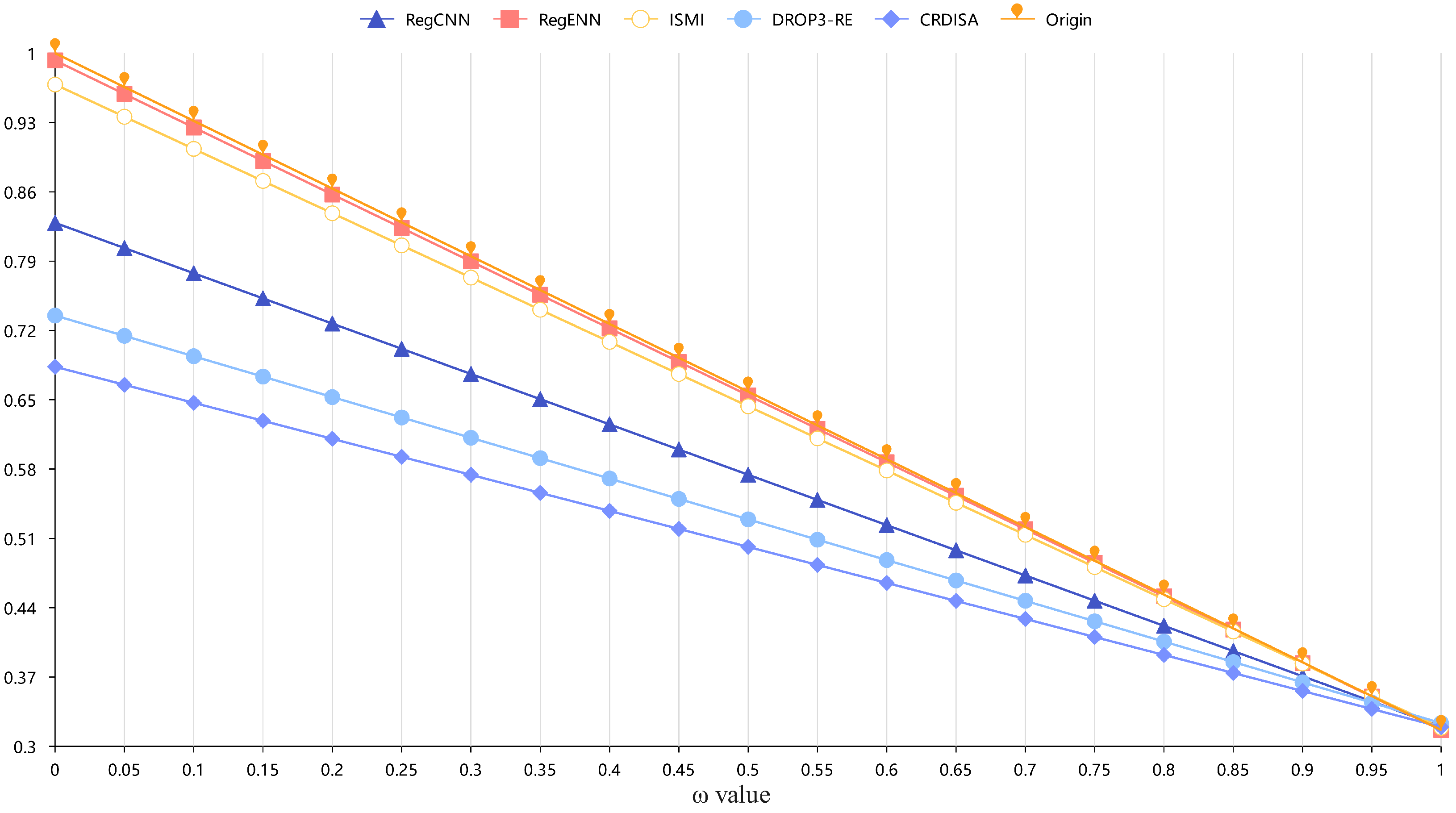
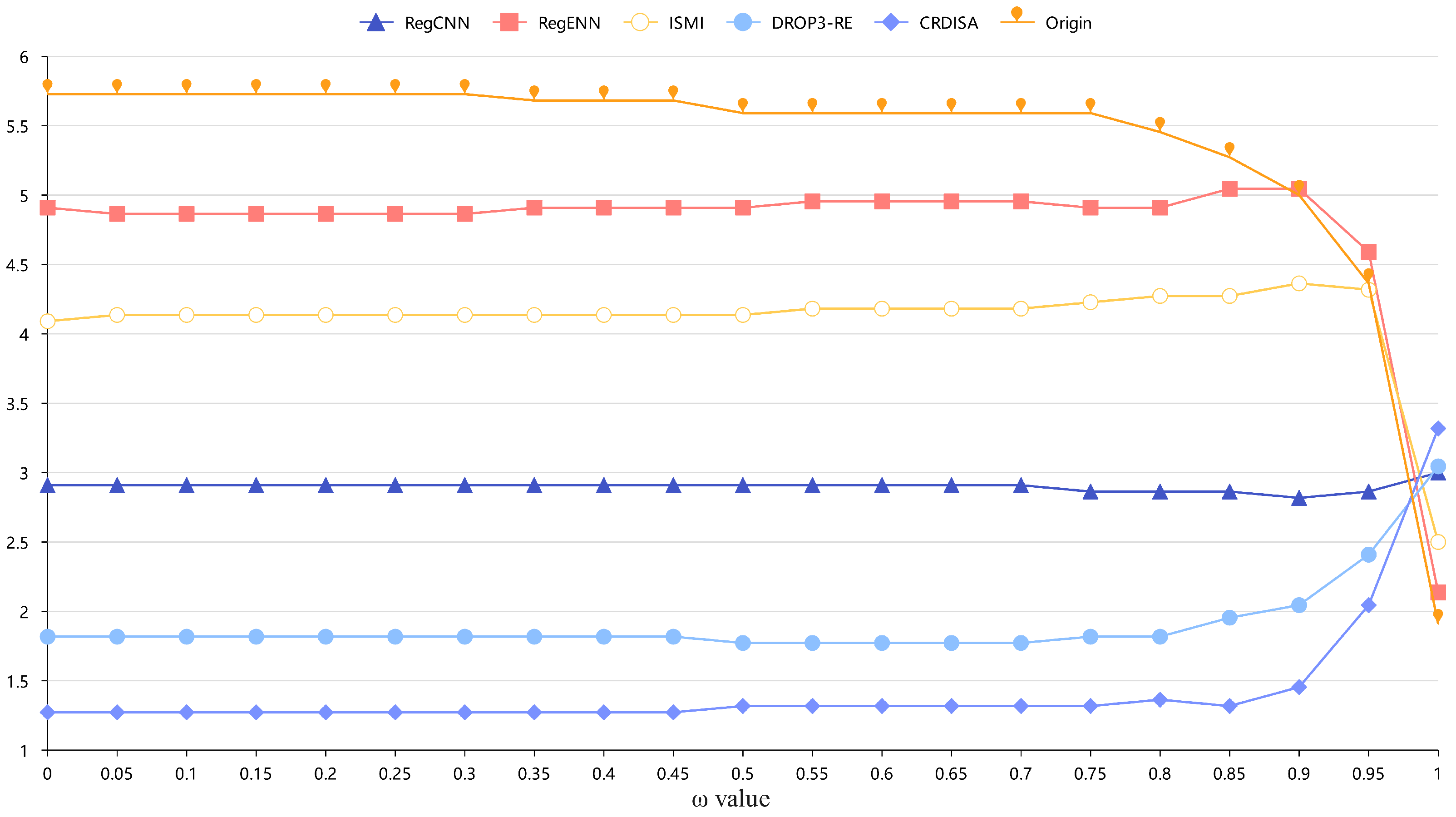
To further quantify this balance between predictive accuracy and compression efficiency, we conducted a comprehensive analysis of the weighted indicator
across varying preference weights
and complemented it with average rank (AR) evaluations (
Figure 10 and
Figure 11,
Table 5).
Consistent with the visual evidence from the Pareto plot, CRDISA dominates the trade-off curve across most weight ranges (particularly for ), delivering the most significant performance gains when balancing accuracy and compression requirements. The average rank analysis further validates CRDISA’s overall superiority: it achieves the lowest average rank of , outperforming DROP3-RE (1.911), RegCNN (2.900), ISMI (4.102), and RegENN (4.771) by a substantial margin. Crucially, the Friedman test confirms the statistical significance of these global ranking differences (), thereby rejecting the null hypothesis of equivalent performance and reinforcing the reliability of the reported rankings.
Notably, this balanced performance is not achieved through a simple accuracy-compression trade-off; instead, it stems from CRDISA’s core innovation—the Difference Knowledge Base, which enables the identification of a minimal sufficient set of Instance Experts. This unique mechanism allows CRDISA to capture the global data distribution far more efficiently than geometry-based competing methods, thereby demonstrating a distinct and robust strength in harmonizing predictive accuracy and compression efficiency across diverse datasets and user preferences.
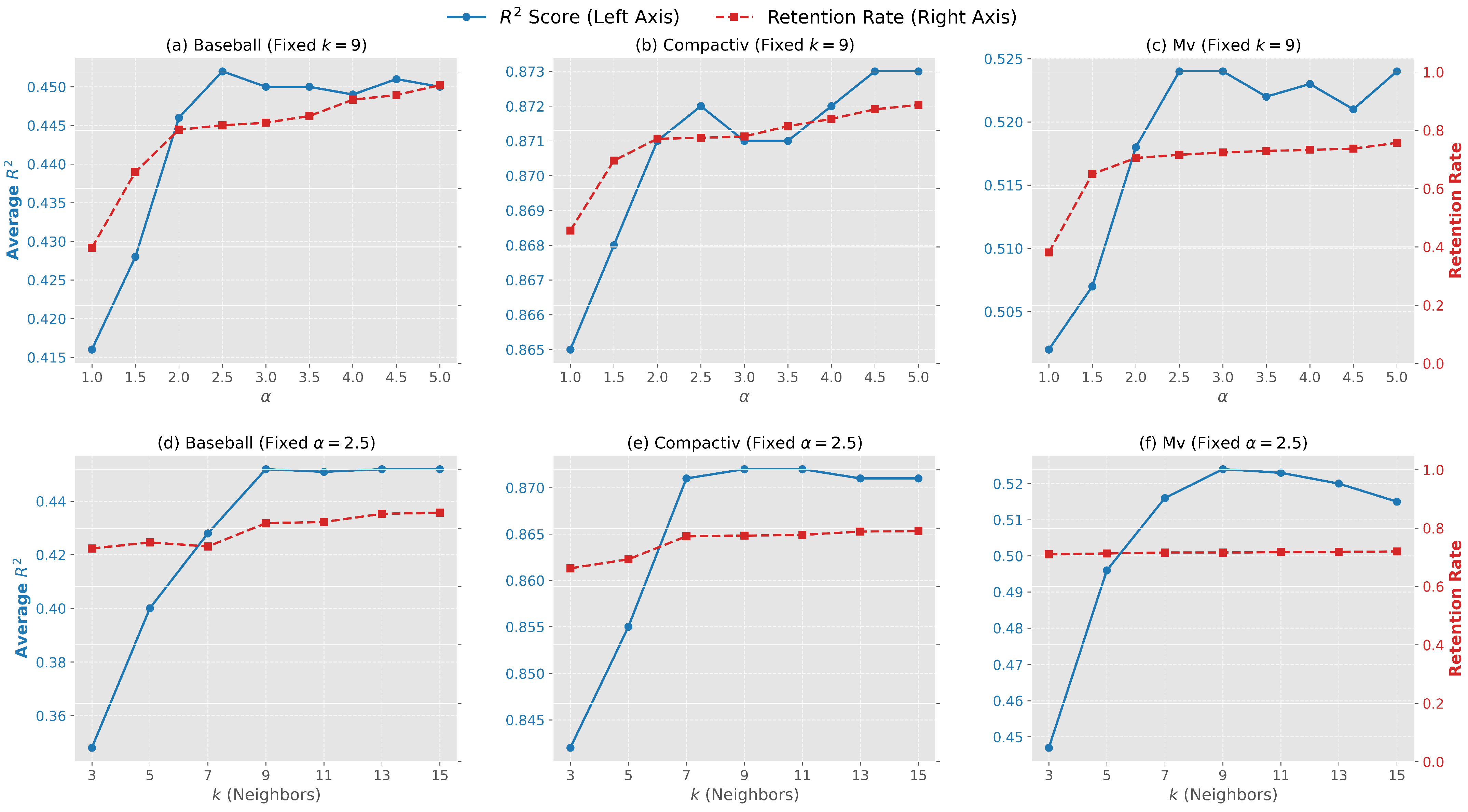
5.2.4. Parameter Sensitivity and Stability Analysis
To empirically justify the admissible range of the sensitivity hyperparameter
and evaluate the stability of the neighborhood size
k, we conducted a comprehensive sensitivity analysis on three representative datasets of varying scales: Baseball, Compactiv, and Mv.
Figure 12 presents the dual-axis evaluation (Accuracy
vs. Retention Rate
m).
(1) Sensitivity to
(
Figure 12, top row): The experimental results reveal a consistent trade-off pattern. In the “Under-fitting Phase” (
), the strict boundary leads to excessive pruning and poor accuracy. As
increases to the range of
, the
score rises sharply and stabilizes at a peak level. This “optimal plateau” empirically validates our default setting, balancing signal retention and noise filtering. Further increasing
(>
) significantly inflates the retention rate without improving accuracy, indicating the inclusion of redundant or noisy instances.
(2) Stability of
k (
Figure 12, bottom row): With
fixed, the analysis of
k exhibits a characteristic “Rise-and-Fall” trend. Performance is unstable at small
k values (
) due to sensitivity to local outliers, while large
k values (
) lead to over-smoothing of local features. A consistent performance peak is observed around
across all datasets, confirming that
is a robust choice for constructing the Difference Knowledge Base.
5.3. Distributed Scalability Analysis
Given the theoretical construction complexity of , proving the scalability of the algorithm is crucial. We conducted stress tests on the MV dataset, scaling instances from 10k to 40k (DS1-DS4) and cores from 10 to 40.
5.3.1. Speedup Analysis
The speedup metric is defined as:
where
denotes the execution time on a single node and
represents the time on
m nodes, with the dataset size kept fixed. Ideally, linear speedup indicates optimal parallel scalability, where doubling the number of nodes halves the execution time.
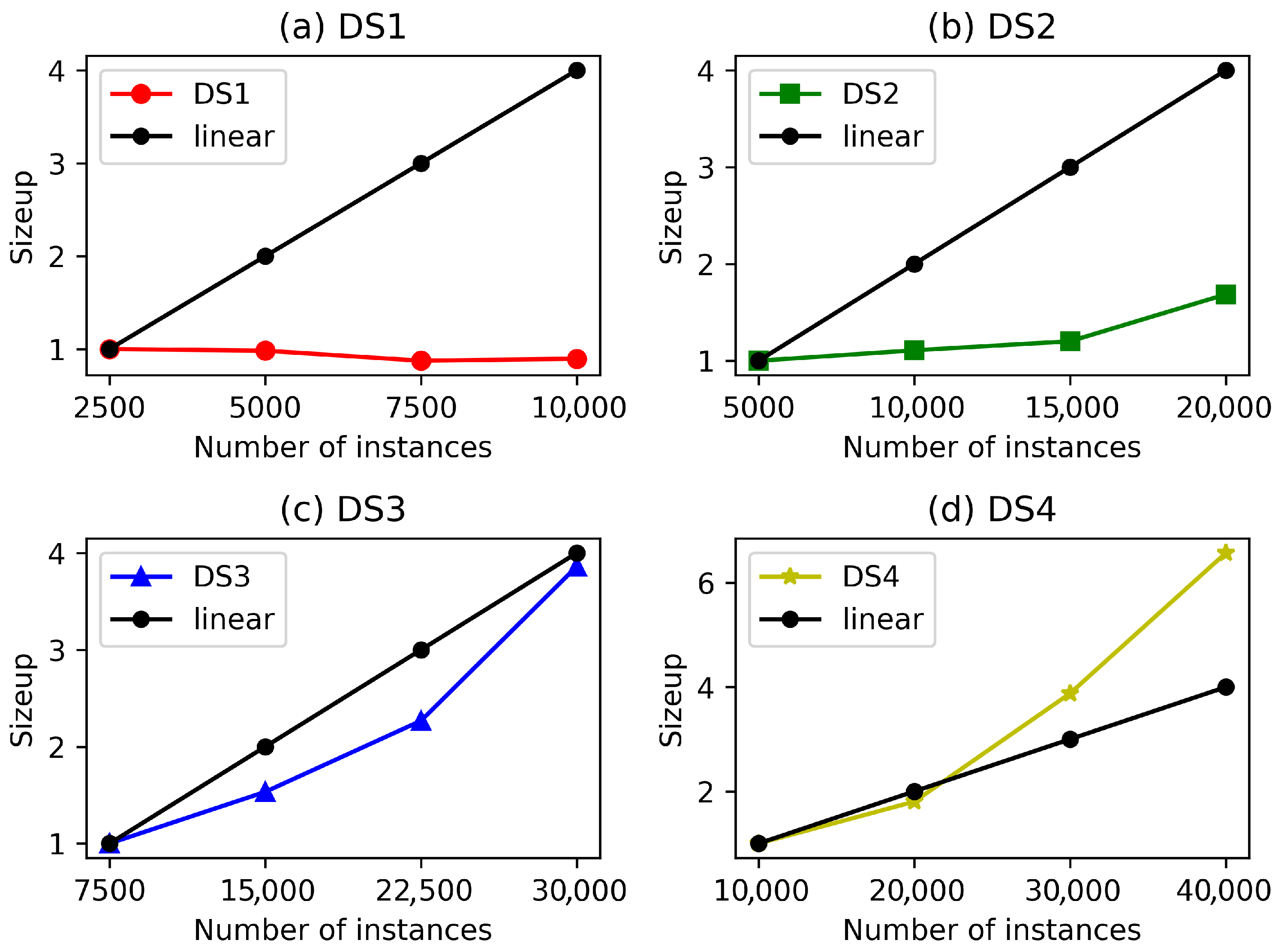
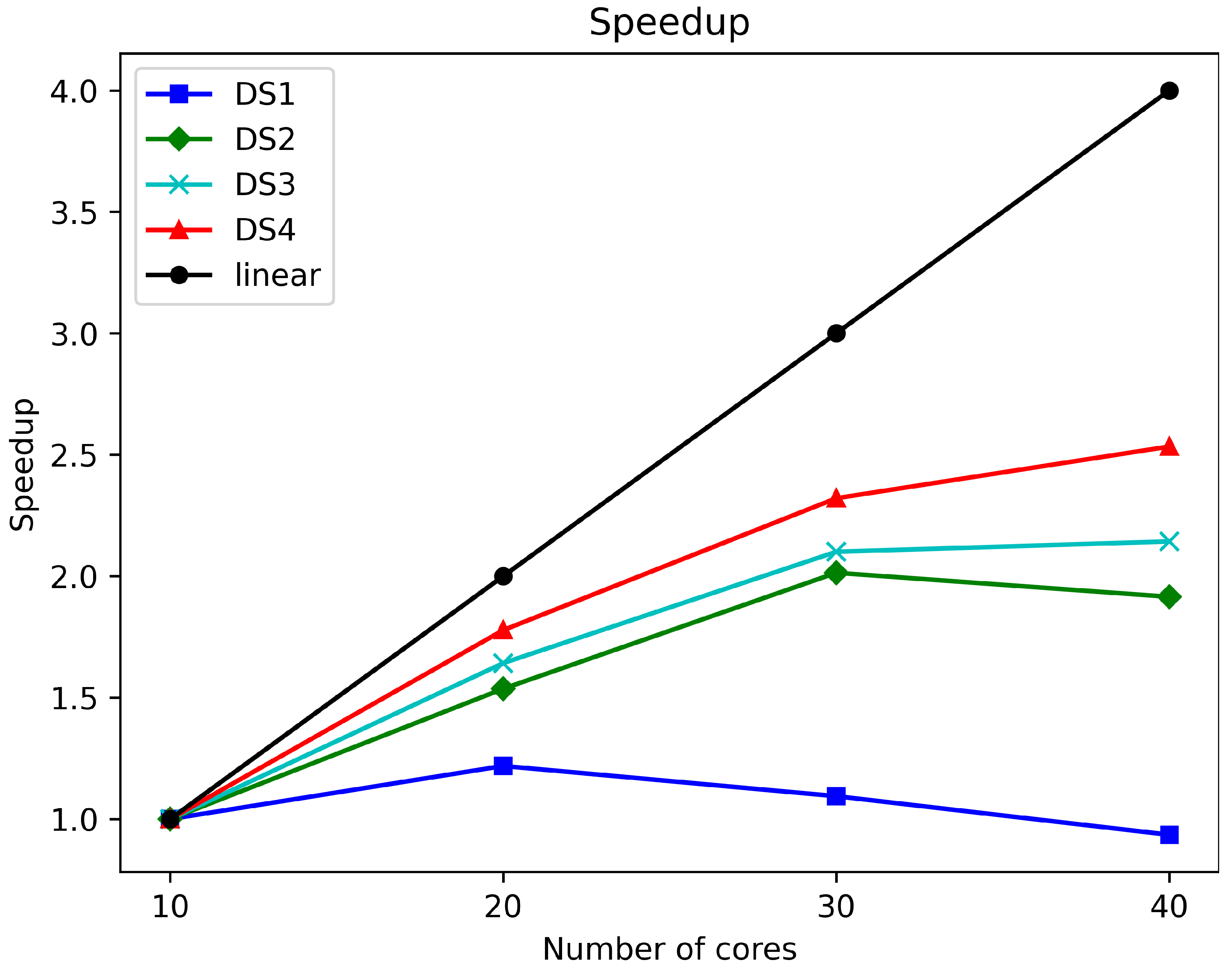
We evaluated CRDISA’s speedup across four datasets (DS1–DS4) using 10, 20, 30, and 40 cores, with results presented in
Figure 13. The experimental results demonstrate that CRDISA achieves near-linear speedup, with the performance gain becoming more pronounced as the dataset size increases. Specifically, for small-scale datasets like DS1, the speedup is sub-linear; this is attributed to the non-negligible overhead from Spark’s DAG scheduling, data distribution, and broadcast serialization, which accounts for a large proportion of the total execution time relative to actual data processing. In contrast, for large datasets such as DS4, the
computational load dominates the
communication overhead, rendering the scheduling and network costs negligible.
Notably, this scalability advantage is underpinned by CRDISA’s Broadcast Optimization strategy (Algorithm 3), which effectively mitigates network bottlenecks. As the workload intensity increases, the optimized broadcast mechanism further reduces communication latency, enabling the system to fully leverage expanded computing resources. In summary, CRDISA exhibits robust parallel scalability with increasing core count, and its performance is more efficient for large-scale datasets—aligning with the demands of big data-driven instance selection tasks.
5.3.2. Sizeup Analysis
The sizeup metric is defined as:
where
denotes the execution time on the original dataset DS, and
represents the time on an
m-fold scaled dataset, with the number of computing nodes fixed at 40 cores. A lower sizeup value indicates a stronger capability to handle large-scale datasets.
To evaluate CRDISA’s sizeup performance, we conducted experiments on datasets scaled to 25%, 50%, 75%, and 100% of their original sizes, with results presented in
Figure 14. The curves reveal a notable trend: for small datasets (e.g., DS1), sizeup remains well below linear growth; as the dataset size expands, however, sizeup exhibits super-linear growth. This behavior is theoretically consistent with Theorem 1, as CRDISA’s quadratic time complexity (
) dictates that doubling the data size quadruples the computational load—primarily stemming from the high cost of constructing difference knowledge bases.
Despite this inherent complexity, CRDISA maintains robust computational stability in practice. Its Spark-based distributed implementation effectively manages the escalating computational load, and crucially, the system operates without memory overflow (OOM) issues. This achievement is attributed to the Uniform Partitioning Strategy (Algorithm 2), which efficiently distributes the memory pressure imposed by difference tensors across computing nodes. In summary, while CRDISA’s sizeup trend reflects its quadratic complexity, its parallel architecture and partitioning optimization ensure satisfactory efficiency for large-scale instance selection tasks.
5.3.3. Scaleup Analysis
The scaleup metric is defined as:
where
m denotes the number of computing nodes. A scaleup value closer to 1 indicates stronger adaptability of the algorithm to varying dataset sizes when computing resources are scaled proportionally.
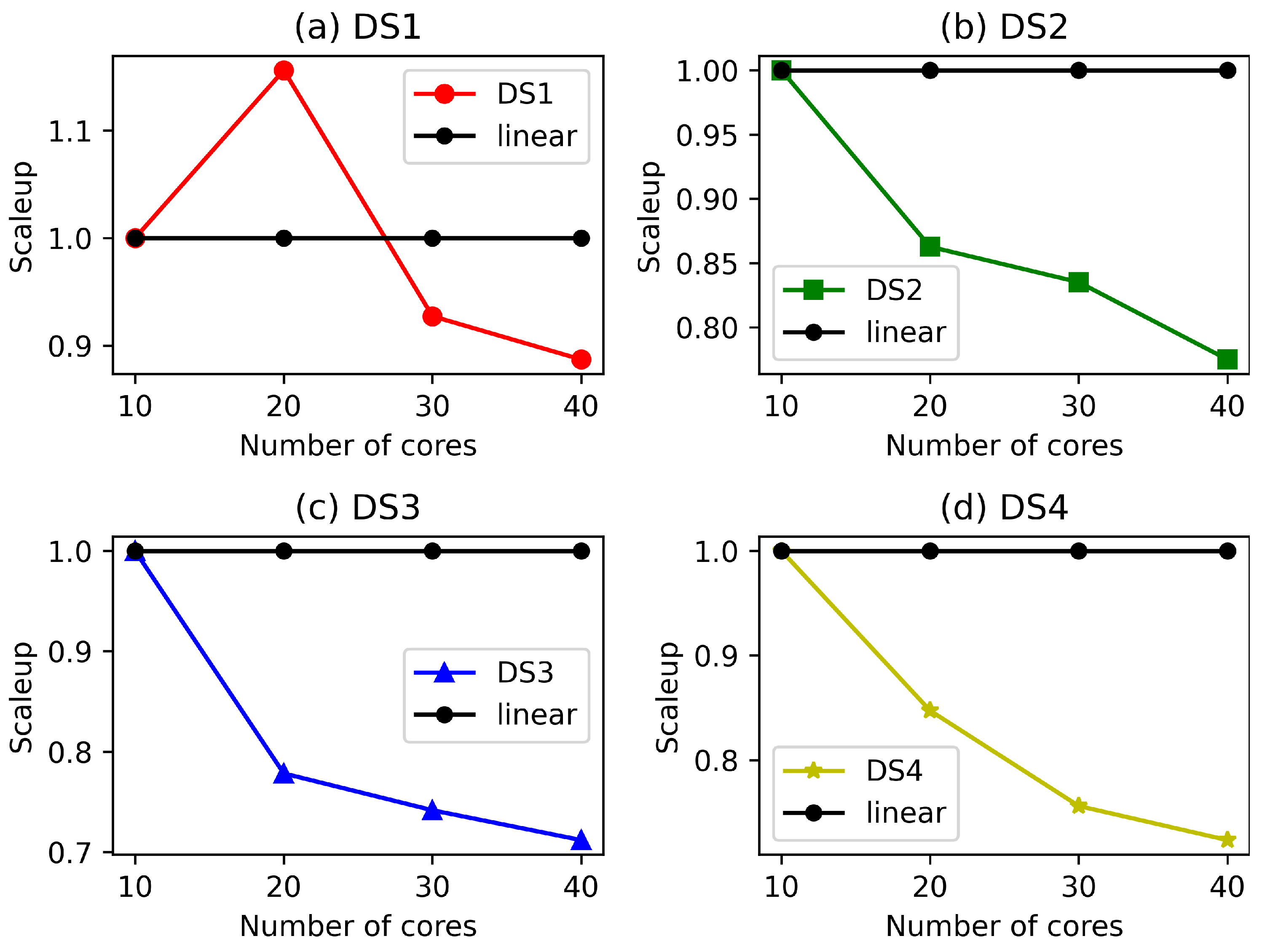
To evaluate CRDISA’s scaleup performance, we processed 20%, 50%, 75%, and 100% of each dataset using 10, 20, 30, and 40 cores respectively, with results presented in
Figure 15. The experimental curves reveal that scaleup exhibits a gradual decline as both dataset size and core count increase—a trend attributed to unavoidable overheads inherent to distributed systems, such as network communication, shuffle operations, and I/O limitations. Notably, however, CRDISA’s scaleup remains consistently above 0.7 across all experimental settings, demonstrating its robust elastic scalability for regression tasks of varying scales.
In practical terms, this distributed architecture allows users to tackle larger regression tasks simply by provisioning additional computing cores, which effectively “buys down” the time cost incurred by the algorithm’s cognitive reasoning process.
6. Conclusions
This paper presents CRDISA, a novel distributed instance selection algorithm that bridges the gap between fine-grained evaluation and parallel scalability in regression tasks. Unlike traditional methods that rely on heuristic subset searches or sequential iterations, CRDISA introduces a rigorous theoretical framework where individual instances are modeled as “Instance Experts.” By endowing instances with the cognitive capability to reason about global data patterns through difference knowledge bases, the algorithm achieves a deterministic and objective assessment of instance quality.
The key contributions of this work are summarized as follows:
Formalization of Cognitive Reasoning: We moved beyond metaphorical descriptions to establish a mathematical definition of “Instance Experts” based on first-order difference vector fields. This paradigm shift allows for the precise, non-heuristic identification of high-quality prototypes, avoiding the local optima and randomness inherent in evolutionary algorithms.
Robust Regression Evaluation Framework: To address the continuity of regression outputs, we proposed a soft partitioning strategy that constructs adaptive error boundaries based on local data variance. Coupled with a bidirectional consensus protocol, this framework effectively filters out noise in validation benchmarks before assessing training instances, ensuring robust selection.
Scalable Distributed Implementation: Acknowledging the computational complexity of constructing knowledge bases, we designed a parallel implementation on Apache Spark. By leveraging uniform partitioning to balance memory loads and an optimized broadcast mechanism to minimize network shuffling, CRDISA effectively mitigates the computational bottleneck, providing linear scalability in execution time relative to the number of executors, thus making the approach suitable for large-scale datasets.
Experimental results on 22 regression datasets demonstrate that CRDISA achieves an average compression rate of 31.7% while maintaining predictive accuracy () comparable to state-of-the-art methods. Its weighted performance rank (1.435) confirms its superiority in balancing accuracy and data reduction. Furthermore, distributed stress tests verify that the algorithm achieves linear speedup and stable scaleup (>0.7), validating its adaptability to growing computational resources.
Limitations and Future Work: Despite its strengths, CRDISA has limitations that define its optimal use cases:
Computational and Memory Costs: While the distributed architecture provides linear scalability in wall-clock time via parallelization, the inherent algorithmic complexity remains in both time and space. For extremely large datasets (e.g., millions of instances), the quadratic memory requirement for storing difference knowledge bases may saturate the cluster’s RAM capacity.
High-Dimensional Sensitivity: The reliance on Euclidean distance within the difference space makes the algorithm sensitive to the “curse of dimensionality,” where distance metrics lose discriminative power in very high-dimensional feature spaces.
Broadcasting Bottleneck: While the current implementation utilizes Spark’s broadcast mechanism to efficiently distribute the validation set and minimize network shuffle, this approach has physical limits (e.g., JVM heap size) when dealing with extremely large datasets. As data volume grows to the terabyte scale, broadcasting the validation set to every node may become infeasible due to memory constraints.
Future work will focus on three directions: (1) integrating Locality-Sensitive Hashing (LSH) to approximate the knowledge base construction. This implies constructing a sparse difference matrix rather than a dense one, effectively reducing both computational and space complexity from to ; (2) incorporating dimensionality reduction techniques (e.g., PCA or Autoencoders) into the preprocessing module to handle high-dimensional data; and (3) addressing the scalability limits for massive datasets by implementing a Distributed Join strategy (e.g., via zipPartitions). This approach will replace the broadcast mechanism in ultra-large-scale scenarios, allowing the validation set to be co-partitioned with training experts to eliminate single-node memory bottlenecks.
In summary, CRDISA offers a theoretically rigorous and mathematically sound approach to instance selection, providing a powerful preprocessing tool for regression tasks in distributed computing environments.
Author Contributions
Conceptualization, L.Y.; methodology, L.Y., W.C. and Z.L.; software, W.C.; validation, W.C.; formal analysis, Z.L. and X.H.; investigation, Z.L.; resources, L.Y.; data curation, W.C.; writing—original draft preparation, L.Y. and W.C.; writing—review and editing, L.Y., X.H. and W.C.; visualization, W.C.; supervision, L.Y.; project administration, L.Y. All authors have read and agreed to the published version of the manuscript.
Funding
This research was funded by National Natural Science Foundation of China, grant number [52307232], and Provincial Natural Science Foundation of Hunan, grant number [2021JJ30877]. The APC was funded by [Central South University].
Institutional Review Board Statement
Not applicable.
Informed Consent Statement
Not applicable.
Data Availability Statement
Conflicts of Interest
The authors declare no conflicts of interest.
References
- Tang, L.; Tian, Y.; Wang, X.; Pardalos, P.M. A simple and reliable instance selection for fast training support vector machine: Valid Border Recognition. Neural Netw. 2023, 166, 379–395. [Google Scholar] [CrossRef]
- Gong, C.; Su, Z.-g.; Wang, P.-h.; Wang, Q.; You, Y. Evidential instance selection for K-nearest neighbor classification of big data. Int. J. Approx. Reason. 2021, 138, 123–144. [Google Scholar] [CrossRef]
- Vitale, F.; Pegoraro, M.; van der Aalst, W.M.; Mazzocca, N. Control-flow anomaly detection by process mining-based feature extraction and dimensionality reduction. Knowl.-Based Syst. 2025, 310, 112970. [Google Scholar] [CrossRef]
- Sowkuntla, P.; Sai Prasad, P. Parallel attribute reduction in high-dimensional data: An efficient MapReduce strategy with fuzzy discernibility matrix. Appl. Soft Comput. 2025, 172, 112870. [Google Scholar] [CrossRef]
- Hadjout, D.; Sebaa, A.; Torres, J.F.; Martínez-Álvarez, F. Electricity consumption forecasting with outliers handling based on clustering and deep learning with application to the Algerian market. Expert Syst. Appl. 2023, 227, 120123. [Google Scholar] [CrossRef]
- Su, Y.; Yang, S.; Liu, Y.; Kai, A.; Chen, L.; Liu, M. Knowledge discovery from porous organic cage literature using a large language model. Digit. Discov. 2025, 4, 43–410. [Google Scholar] [CrossRef]
- Chen, R.; Jing, X.Y.; Wu, F.; Chen, H. Sharpness-aware gradient guidance for few-shot class-incremental learning. Knowl.-Based Syst. 2024, 299, 112030. [Google Scholar] [CrossRef]
- Xiong, L.; Guan, X.; Xiong, H.; Zhu, K.; Zhang, F. Knowledge fusion distillation and gradient-based data distillation for class-incremental learning. Neurocomputing 2025, 622, 129286. [Google Scholar] [CrossRef]
- Liu, Y.; Du, G.; Yin, C.; Zhang, H.; Wang, J. Clustering-based incremental learning for imbalanced data classification. Knowl.-Based Syst. 2024, 292, 111612. [Google Scholar] [CrossRef]
- Ozay, D.; Jahanbakth, M.; Wang, S. Exploring the Intersection of Big Data and AI With CRM Through Descriptive, Network, and Contextual Methods. IEEE Access 2025, 13, 57223–57240. [Google Scholar] [CrossRef]
- Kordos, M.; Blachnik, M. Instance Selection with Neural Networks for Regression Problems. In Artificial Neural Networks and Machine Learning—ICANN 2012, Proceedings of the Conference on Artificial Neural Networks, Lausanne, Switzerland, 11–14 September 2012; Villa, A.E.P., Duch, W., Érdi, P., Masulli, F., Palm, G., Eds.; Springer: Berlin/Heidelberg, Germany, 2012; pp. 263–270. [Google Scholar] [CrossRef]
- Xu, C.; Zhang, S. A Genetic Algorithm-based sequential instance selection framework for ensemble learning. Expert Syst. Appl. 2024, 236, 121269. [Google Scholar] [CrossRef]
- Cao, Y.; Zhou, Z.J.; Hu, C.H.; Tang, S.W.; Wang, J. A new approximate belief rule base expert system for complex system modelling. Decis. Support Syst. 2021, 150, 113558. [Google Scholar] [CrossRef]
- Olvera-López, J.A.; Carrasco-Ochoa, J.A.; Martínez-Trinidad, J.F.; Kittler, J. A review of instance selection methods. Artif. Intell. Rev. 2010, 34, 133–143. [Google Scholar] [CrossRef]
- Wilson, D.R.; Martinez, T.R. Reduction Techniques for Instance-Based Learning Algorithms. Mach. Learn. 2000, 38, 257–286. [Google Scholar] [CrossRef]
- Yeo, G.F.A.; Hudson, I.; Akman, D.; Chan, J. SpIS: A stochastic approximation approach to minimal subset instance selection. Inf. Sci. 2025, 695, 121738. [Google Scholar] [CrossRef]
- Yeo, G.F.A.; Akman, D.; Hudson, I.; Chan, J. A stochastic approximation approach to fixed instance selection. Inf. Sci. 2023, 628, 558–579. [Google Scholar] [CrossRef]
- Qin, L.; Wang, X.; Yin, L.; Jiang, Z. A distributed evolutionary based instance selection algorithm for big data using Apache Spark. Appl. Soft Comput. 2024, 159, 111638. [Google Scholar] [CrossRef]
- Cheng, F.; Chu, F.; Zhang, L. A multi-objective evolutionary algorithm based on length reduction for large-scale instance selection. Inf. Sci. 2021, 576, 105–121. [Google Scholar] [CrossRef]
- Riquelme, J.C.; Aguilar-Ruiz, J.S.; Toro, M. Finding representative patterns with ordered projections. Pattern Recognit. 2003, 36, 1009–1018. [Google Scholar] [CrossRef]
- Raicharoen, T.; Lursinsap, C. A divide-and-conquer approach to the pairwise opposite class-nearest neighbor (POC-NN) algorithm. Pattern Recognit. Lett. 2005, 26, 1554–1567. [Google Scholar] [CrossRef]
- Garcia, S.; Derrac, J.; Cano, J.; Herrera, F. Prototype Selection for Nearest Neighbor Classification: Taxonomy and Empirical Study. IEEE Trans. Pattern Anal. Mach. Intell. 2012, 34, 417–435. [Google Scholar] [CrossRef] [PubMed]
- Arnaiz-González, Á.; Blachnik, M.; Kordos, M.; García-Osorio, C. Fusion of instance selection methods in regression tasks. Inf. Fusion 2016, 30, 69–79. [Google Scholar] [CrossRef]
- Antonelli, M.; Ducange, P.; Marcelloni, F. Genetic Training Instance Selection in Multiobjective Evolutionary Fuzzy Systems: A Coevolutionary Approach. IEEE Trans. Fuzzy Syst. 2012, 20, 276–290. [Google Scholar] [CrossRef]
- Kordos, M.; Łapa, K. Multi-Objective Evolutionary Instance Selection for Regression Tasks. Entropy 2018, 20, 746. [Google Scholar] [CrossRef]
- García-Pedrajas, N.; Romero del Castillo, J.A.; Ortiz-Boyer, D. A cooperative coevolutionary algorithm for instance selection for instance-based learning. Mach. Learn. 2010, 78, 381–420. [Google Scholar] [CrossRef]
- Kordos, M.; Blachnik, M.; Scherer, R. Fuzzy clustering decomposition of genetic algorithm-based instance selection for regression problems. Inf. Sci. 2022, 587, 23–40. [Google Scholar] [CrossRef]
- Arnaiz-González, Á.; Díez-Pastor, J.F.; Rodríguez, J.J.; García-Osorio, C.I. Instance selection for regression by discretization. Expert Syst. Appl. 2016, 54, 340–350. [Google Scholar] [CrossRef]
- Song, Y.; Liang, J.; Lu, J.; Zhao, X. An efficient instance selection algorithm for k nearest neighbor regression. Neurocomputing 2017, 251, 26–34. [Google Scholar] [CrossRef]
- Guillen, A.; Herrera, L.; Rubio, G.; Pomares, H.; Lendasse, A.; Rojas, I. New method for instance or prototype selection using mutual information in time series prediction. Neurocomputing 2010, 73, 2030–2038. [Google Scholar] [CrossRef]
- Arnaiz-González, Á.; Díez-Pastor, J.F.; Rodríguez, J.J.; García-Osorio, C. Instance selection for regression: Adapting DROP. Neurocomputing 2016, 201, 66–81. [Google Scholar] [CrossRef]
- Li, C.; Zhang, Y.; Luo, Y. Intermediate data placement and cache replacement strategy under Spark platform. J. Parallel Distrib. Comput. 2022, 163, 114–135. [Google Scholar] [CrossRef]
- Yin, L.; Cao, K.; Jiang, Z.; Li, Z. RA-MRS: A high efficient attribute reduction algorithm in big data. J. King Saud Univ.-Comput. Inf. Sci. 2024, 36, 102064. [Google Scholar] [CrossRef]
- Zhang, F.; Zhai, J.; Shen, X.; Mutlu, O.; Du, X. POCLib: A High-Performance Framework for Enabling Near Orthogonal Processing on Compression. IEEE Trans. Parallel Distrib. Syst. 2022, 33, 459–475. [Google Scholar] [CrossRef]
- Ahmed, E.M. Big Data Analytics Implications on Central Banking Green Technological Progress. Int. J. Inf. Technol. Decis. Mak. 2024, 23, 2065–2087. [Google Scholar] [CrossRef]
- Yin, L.; Qin, L.; Jiang, Z.; Xu, X. A fast parallel attribute reduction algorithm using Apache Spark. Knowl.-Based Syst. 2021, 212, 106582. [Google Scholar] [CrossRef]
- Alcala-Fdez, J.; Fernández, A.; Luengo, J.; Derrac, J.; Garc’ia, S.; Sanchez, L.; Herrera, F. KEEL Data-Mining Software Tool: Data Set Repository, Integration of Algorithms and Experimental Analysis Framework. J. Mult.-Valued Log. Soft Comput. 2010, 17, 255–287. [Google Scholar]
- Holm, S. A Simple Sequentially Rejective Multiple Test Procedure. Scand. J. Stat. 1979, 6, 65–70. [Google Scholar]
Figure 1.
The core concept of CRDISA. The workflow integrates cognitive empowerment (“Instance Expert” construction), soft boundary establishment, reasoning evaluation, and the bidirectional voting.
Figure 1.
The core concept of CRDISA. The workflow integrates cognitive empowerment (“Instance Expert” construction), soft boundary establishment, reasoning evaluation, and the bidirectional voting.
Figure 2.
Construction process of the difference knowledge base. Each instance computes difference vectors with the entire dataset to form its unique cognitive domain.
Figure 2.
Construction process of the difference knowledge base. Each instance computes difference vectors with the entire dataset to form its unique cognitive domain.
Figure 3.
Soft boundary calculation for instances in the validation set. The boundary adapts to the standard deviation of the local neighborhood.
Figure 3.
Soft boundary calculation for instances in the validation set. The boundary adapts to the standard deviation of the local neighborhood.
Figure 4.
Evaluation process of reasoning results. Predictions are compared against soft boundaries to populate the binary evaluation matrix.
Figure 4.
Evaluation process of reasoning results. Predictions are compared against soft boundaries to populate the binary evaluation matrix.
Figure 5.
Principle of the bidirectional consensus protocol. The mechanism first filters validation instances (columns) and then selects training instances (rows) based on the updated matrix.
Figure 5.
Principle of the bidirectional consensus protocol. The mechanism first filters validation instances (columns) and then selects training instances (rows) based on the updated matrix.
Figure 8.
Heatmap comparison of Retention Rates (m) across 22 datasets. The color intensity represents the magnitude of the retention rate. CRDISA consistently exhibits superior compression performance (distinct color column) across diverse datasets compared to baselines.
Figure 8.
Heatmap comparison of Retention Rates (m) across 22 datasets. The color intensity represents the magnitude of the retention rate. CRDISA consistently exhibits superior compression performance (distinct color column) across diverse datasets compared to baselines.
Figure 9.
Accuracy () vs. Retention Rate (m) Trade-off Analysis. The scatter points represent the mean performance of each algorithm across 22 datasets. CRDISA (red star) occupies the optimal “sweet spot” in the top-left corner, demonstrating a dominant balance between high accuracy and low data retention compared to other algorithms.
Figure 9.
Accuracy () vs. Retention Rate (m) Trade-off Analysis. The scatter points represent the mean performance of each algorithm across 22 datasets. CRDISA (red star) occupies the optimal “sweet spot” in the top-left corner, demonstrating a dominant balance between high accuracy and low data retention compared to other algorithms.
Figure 10.
The trend of Weighted Indicator with varying .
Figure 10.
The trend of Weighted Indicator with varying .
Figure 11.
The trend of Average Rank (AR) with varying .
Figure 11.
The trend of Average Rank (AR) with varying .
Figure 12.
Parameter sensitivity and stability analysis on three representative datasets: Baseball (Small), Compactiv (Medium), and Mv (Large). The top row (a–c) illustrates the impact of the adaptive boundary factor (with fixed ) on predictive accuracy (, left axis) and retention rate (m, right axis). The bottom row (d–f) displays the stability of the neighborhood size k (with fixed ). The results confirm an optimal operating range of and a stable neighborhood size of across varying data scales.
Figure 12.
Parameter sensitivity and stability analysis on three representative datasets: Baseball (Small), Compactiv (Medium), and Mv (Large). The top row (a–c) illustrates the impact of the adaptive boundary factor (with fixed ) on predictive accuracy (, left axis) and retention rate (m, right axis). The bottom row (d–f) displays the stability of the neighborhood size k (with fixed ). The results confirm an optimal operating range of and a stable neighborhood size of across varying data scales.
Figure 13.
Speedup analysis across varying dataset sizes and core counts.
Figure 13.
Speedup analysis across varying dataset sizes and core counts.
Figure 14.
Sizeup analysis.
Figure 14.
Sizeup analysis.
Figure 15.
Scaleup analysis.
Figure 15.
Scaleup analysis.
Table 1.
Theoretical Comparison of Instance Selection Frameworks.
Table 1.
Theoretical Comparison of Instance Selection Frameworks.
| Feature | Traditional Instance Selection (e.g., RegCNN) | Proposed CRDISA |
|---|
| Operational Paradigm | Passive Filtering: Instances are kept/removed by external algorithms based on global rules. | Active Reasoning: Each instance acts as an independent expert (“Agent”) that evaluates itself. |
| Search Space | Original Feature Space (): Euclidean distance between static points. | Difference Vector Space (): Similarity of relational shifts. |
| Selection Criteria | Geometric Centrality: Retains boundary or central points based on statistical error. | Generalization Capability: Retains instances based on their ability to predict unseen targets. |
Table 2.
Description of 22 regression datasets.
Table 2.
Description of 22 regression datasets.
| Dataset | Abbrev. | Features | Instances | Original |
|---|
| MachineCPU | MAC | 6 | 209 | 0.713 |
| Baseball | BAS | 16 | 337 | 0.456 |
| Dee | DEE | 6 | 365 | 0.797 |
| AutoMPG6 | AU6 | 5 | 392 | 0.703 |
| AutoMPG8 | AU8 | 7 | 392 | 0.711 |
| Ele-1 | EL1 | 2 | 495 | 0.689 |
| Stock | STO | 9 | 950 | 0.983 |
| Treasury | TRE | 15 | 1049 | 0.983 |
| Mortgage | MOR | 15 | 1049 | 0.989 |
| Ele-2 | EL2 | 4 | 1056 | 0.993 |
| Wizmir | WIZ | 9 | 1461 | 0.990 |
| Airfoil | AIR | 5 | 1503 | 0.247 |
| Wankara | WAN | 9 | 1609 | 0.991 |
| Plastic | PLA | 2 | 1650 | 0.769 |
| Delta_ail | AIL | 5 | 7129 | 0.608 |
| Compactiv | COM | 21 | 8192 | 0.872 |
| Puma32h | PUM | 32 | 8192 | 0.132 |
| Delta_elv | ELV | 6 | 9517 | 0.540 |
| CCPP | CCP | 4 | 9568 | 0.946 |
| California | CAL | 8 | 20,640 | 0.304 |
| House | HOU | 16 | 22,784 | 0.078 |
| Mv | MV | 10 | 40,768 | 0.543 |
Table 3.
comparison across algorithms.
Table 3.
comparison across algorithms.
| Dataset | RegCNN | RegENN | ISMI | DROP3-RE | CRDISA |
|---|
| MAC | 0.708 | 0.709 | 0.710 | 0.727 | 0.709 |
| BAS | 0.447 | 0.452 | 0.439 | 0.449 | 0.452 |
| DEE | 0.793 | 0.795 | 0.795 | 0.793 | 0.801 |
| AU6 | 0.704 | 0.705 | 0.698 | 0.696 | 0.700 |
| AU8 | 0.703 | 0.714 | 0.704 | 0.694 | 0.701 |
| EL1 | 0.677 | 0.687 | 0.682 | 0.678 | 0.673 |
| STO | 0.979 | 0.983 | 0.983 | 0.983 | 0.980 |
| TRE | 0.982 | 0.983 | 0.982 | 0.982 | 0.979 |
| MOR | 0.987 | 0.989 | 0.989 | 0.990 | 0.981 |
| EL2 | 0.993 | 0.993 | 0.993 | 0.994 | 0.993 |
| WIZ | 0.990 | 0.990 | 0.990 | 0.990 | 0.988 |
| AIR | 0.246 | 0.245 | 0.249 | 0.221 | 0.276 |
| WAN | 0.991 | 0.991 | 0.991 | 0.991 | 0.991 |
| PLA | 0.775 | 0.769 | 0.767 | 0.779 | 0.778 |
| AIL | 0.608 | 0.606 | 0.607 | 0.605 | 0.601 |
| COM | 0.872 | 0.872 | 0.873 | 0.817 | 0.872 |
| PUM | 0.124 | 0.132 | 0.134 | 0.107 | 0.133 |
| ELV | 0.538 | 0.538 | 0.539 | 0.528 | 0.526 |
| CCP | 0.945 | 0.946 | 0.946 | 0.945 | 0.943 |
| CAL | 0.299 | 0.305 | 0.305 | 0.295 | 0.289 |
| HOU | 0.057 | 0.095 | 0.073 | 0.090 | 0.085 |
| MV | 0.544 | 0.541 | 0.541 | 0.530 | 0.524 |
| Average | 0.680 | 0.684 | 0.681 | 0.677 | 0.681 |
| Wilcoxon P | 0.643 | 0.055 | 0.360 | 0.781 | |
Table 4.
m comparison across algorithms.
Table 4.
m comparison across algorithms.
| Dataset | RegCNN | RegENN | ISMI | DROP3-RE | CRDISA |
|---|
| MAC | 0.870 | 0.980 | 0.972 | 0.752 | 0.735 |
| BAS | 0.837 | 0.980 | 0.944 | 0.689 | 0.817 |
| DEE | 0.842 | 0.991 | 0.942 | 0.749 | 0.791 |
| AU6 | 0.853 | 0.991 | 0.951 | 0.739 | 0.527 |
| AU8 | 0.842 | 0.990 | 0.943 | 0.738 | 0.662 |
| EL1 | 0.847 | 0.998 | 0.947 | 0.725 | 0.800 |
| STO | 0.846 | 1.000 | 0.947 | 0.820 | 0.808 |
| TRE | 0.788 | 0.998 | 0.981 | 0.861 | 0.727 |
| MOR | 0.787 | 1.000 | 0.988 | 0.870 | 0.618 |
| EL2 | 0.762 | 1.000 | 0.996 | 0.735 | 0.699 |
| WIZ | 0.746 | 0.999 | 0.963 | 0.717 | 0.440 |
| AIR | 0.821 | 0.999 | 0.972 | 0.736 | 0.672 |
| WAN | 0.759 | 1.000 | 0.957 | 0.718 | 0.561 |
| PLA | 0.870 | 1.000 | 0.960 | 0.626 | 0.540 |
| AIL | 0.838 | 0.984 | 0.999 | 0.665 | 0.694 |
| COM | 0.843 | 0.991 | 0.979 | 0.685 | 0.774 |
| PUM | 0.868 | 1.000 | 0.961 | 0.690 | 0.600 |
| ELV | 0.840 | 0.991 | 0.996 | 0.706 | 0.769 |
| CCP | 0.832 | 0.995 | 0.993 | 0.751 | 0.717 |
| CAL | 0.863 | 0.995 | 0.986 | 0.738 | 0.668 |
| HOU | 0.832 | 0.962 | 0.961 | 0.707 | 0.698 |
| MV | 0.845 | 0.994 | 0.966 | 0.755 | 0.716 |
| Average | 0.829 | 0.993 | 0.968 | 0.735 | 0.683 |
| Wilcoxon P | 4.77 × | 4.77 × | 4.77 × | 0.046 | |
Table 5.
The overall performance ranking of the 5 algorithms.
Table 5.
The overall performance ranking of the 5 algorithms.
| Algorithm | RegCNN | RegENN | ISMI | DROP3-RE | CRDISA |
|---|
| Ranking | 2.900 | 4.771 | 4.102 | 1.911 | 1.435 |
| Disclaimer/Publisher’s Note: The statements, opinions and data contained in all publications are solely those of the individual author(s) and contributor(s) and not of MDPI and/or the editor(s). MDPI and/or the editor(s) disclaim responsibility for any injury to people or property resulting from any ideas, methods, instructions or products referred to in the content. |