GeoMIP: A Geometric-Topological and Dynamic Programming Framework for Enhanced Computational Tractability of Minimum Information Partition in Integrated Information Theory

Abstract

The computational tractability of Integrated Information Theory (IIT) is fundamentally constrained by the exponential cost of identifying the Minimum Information Partition (MIP), which is required to quantify integrated information (Φ). Existing approaches become impractical beyond ~15–20 variables, limiting IIT analyses on realistic neural and complex systems. We introduce GeoMIP, a geometric–topological framework that recasts the MIP search as a graph-based optimization problem on the n-dimensional hypercube graph: discrete system states are modeled as graph vertices, and Hamming distance adjacency defines edges and shortest-path structures. Building on a tensor-decomposed representation of the transition probabilities, GeoMIP constructs a transition-cost (ground cost) structure by dynamic programming over graph neighborhoods and BFS-like exploration by Hamming levels, exploiting hypercube symmetries to reduce redundant evaluations. We validate GeoMIP against PyPhi, ensuring reliability of MIP identification and Φ computation. Across multiple implementations, GeoMIP achieves 165–326× speedups over PyPhi while maintaining 98–100% agreement in partition identification. Heuristic extensions further enable analyses up to ~25 variables, substantially expanding the practical IIT regime. Overall, by leveraging the hypercube’s explicit graph structure (vertices, edges, shortest paths, and automorphisms), GeoMIP turns an intractable combinatorial search into a scalable graph-based procedure for IIT partitioning.

1. Introduction

1.1. The Challenge of Consciousness Quantification

The scientific investigation of consciousness represents one of the most profound challenges in contemporary neuroscience and cognitive science. While advances in neuroimaging and computational neuroscience have enabled unprecedented insights into neural correlates of consciousness, fundamental questions regarding the emergence, nature, and quantification of conscious experience remain largely unresolved [1]. The transition from identifying mere correlations between neural activity and conscious states to establishing causal mechanisms underlying consciousness requires theoretical frameworks capable of quantifying conscious phenomena in precise, mathematical terms.

Integrated Information Theory (IIT), originally formulated by Tononi [2] and subsequently refined through multiple iterations [3,4] culminating in IIT 4.0 [5,6,7], represents a paradigmatic attempt to address this challenge by proposing that consciousness corresponds to integrated information (Φ) generated by a system. According to IIT’s foundational postulates, consciousness is not merely an emergent property of complex neural dynamics but constitutes an intrinsic aspect of systems capable of generating unified, irreducible information about their own states [4]. This theoretical framework has gained substantial traction in consciousness research due to its mathematical rigor and empirical testability, providing quantitative predictions about consciousness levels across different systems and states [8].

1.2. The Computational Challenge

The theory’s mathematical formalism relies critically on identifying the Minimum Information Partition (MIP), which determines how a system should be divided to minimize the loss of integrated information. This partition reveals the system’s causal structure and quantifies its irreducibility—fundamental properties that distinguish conscious from unconscious processing [6].

The computational challenge of MIP determination stems from the exponential growth of possible system partitions. For a subsystem containing u elements at time t and v elements at time t + 1, the number of possible bipartitions scales as 2^(u+v−1) − 1, creating an intractable search space for realistic neural networks [9]. The computational determination of MIP has emerged as the primary bottleneck limiting IIT’s practical applicability [10,11], constraining analyses to idealized systems with fewer than 20–25 variables [12]. This combinatorial explosion means that analysis times grow from milliseconds for small systems to years for systems with 32 variables, effectively precluding analysis of realistic neural circuits (see Table 1).

Table 1. Analysis times grow and search space.

System Size	Partitions Number	Estimated Time
4	7	Milliseconds
8	127	Seconds
16	32.767	Hours
32	~2.1 Billions	Years

Current methodologies face insurmountable computational barriers when analyzing systems with more than 15–20 variables, severely limiting the practical applicability of IIT to realistic neural networks and complex systems.

1.3. State of the Art

Recent systematic reviews of computational methods in Integrated Information Theory have categorized existing approaches into distinct families addressing the fundamental MIP identification challenge [11]. The foundational implementation PyPhi [13] established rigorous computational standards but remained limited by exhaustive search requirements, becoming computationally prohibitive for systems exceeding 15–20 variables due to exponential scaling of the partition search space.

Optimization approaches have explored various strategies to address these limitations: submodular optimization techniques that exploit mathematical properties of specific distance functions [10], achieving performance improvements but remaining fundamentally constrained by exponential search space complexity [9]. These approaches typically require restrictive assumptions about mathematical structure that may not hold for general biological systems.

Approximation and heuristic methods have been developed, trading computational tractability for solution accuracy through random sampling, greedy optimization, and constraint relaxation [14]. While these approaches can handle larger systems, they typically sacrifice the mathematical precision fundamental to IIT’s theoretical foundations, potentially compromising consciousness quantification validity.

Current methods range from exhaustive search implementations (PyPhi) that provide perfect accuracy but remain computationally limited to approximately 12–15 nodes due to O(2^N exponential complexity, to submodular optimization approaches (Queyranne’s algorithm) achieving O(N³) polynomial complexity for symmetric functions but constrained to specific mathematical structures and ineffective beyond N > 100. Alternative strategies include stochastic approximation methods (REMCMC) enabling exploration of non-submodular measures with O(TN²) complexity but requiring high computational costs and sensitivity to initial conditions, graph-theoretic approaches achieving search space reduction through spectral clustering while producing approximate rather than optimal solutions, and thermodynamic approximation methods employing kinetic Ising models for scalability at the cost of simplified assumptions limiting generalizability to complex biological systems [11].

The systematic analysis identifies a critical computational gap where existing methods either maintain theoretical accuracy while sacrificing scalability (exhaustive approaches) or achieve computational tractability while compromising precision (approximation methods), with practical barriers limiting current implementations to idealized systems with minimal units [12]. Within this landscape, GeoMIP represents a novel geometric-topological paradigm that exploits inherent structural properties of discrete systems to transcend traditional optimization constraints. Unlike approximation methods that sacrifice precision for efficiency, or exact methods that lack scalability, the geometric reformulation achieves both computational tractability and theoretical rigor through fundamental mathematical insight rather than algorithmic compromise, extending practical IIT analysis from systems with ≤15 variables to systems with 20–25+ variables while maintaining perfect accuracy in consciousness quantification.

Recent developments in IIT 4.0 have introduced refined mathematical formalisms that better capture the relationship between causal structure and conscious experience [7]. This latest formulation emphasizes the intrinsic existence of conscious systems and introduces new measures of system integrated information such as φ*s (maximal system integrated information) and formal frameworks for analyzing cause-effect relationships [15] that identify conscious entities as those achieving maximal irreducibility [16]. However, these advances have paradoxically increased computational demands, as the expanded formalism requires even more intensive calculations for practical implementation. The resulting computational bottleneck has been identified as a critical barrier to empirical validation of IIT’s theoretical predictions [17].

1.4. Research Contributions

This research introduces GeoMIP, a novel geometric-topological framework that fundamentally reconceptualizes the MIP problem by exploiting the natural correspondence between discrete system states and hypercube geometry. Our approach transforms the traditional combinatorial search into a structured geometric analysis, leveraging tensor decomposition, recursive cost functions, and topological invariances to achieve unprecedented computational efficiency while maintaining theoretical rigor. The primary contributions of this work include:

(a) Geometric-topological reformulation: The development of a comprehensive mathematical framework that maps discrete state spaces to hypercube geometry, revealing previously hidden structural relationships that enable efficient MIP determination. This includes a novel recursive cost function that exploits Hamming distance properties and geometric invariances to quantify transition energies within the hypercube structure.

(b) Algorithmic breakthrough: A complete framework achieving substantial computational improvements through dynamic programming, topological optimization, and tensor decomposition while maintaining theoretical guarantees.

(c) Empirical validation: The validation demonstrates speedups of 165–326× over current state-of-the-art methods while maintaining 98–100% accuracy in partition identification and Φ value calculation. These results establish GeoMIP as both theoretically sound and practically superior to existing approaches, providing compelling evidence for the utility of geometric methods in consciousness research. The validation encompasses diverse system configurations and rigorous performance metrics to ensure robust assessment of the methodology’s capabilities.

The application of geometric and topological methods to complex computational problems has yielded remarkable advances across diverse scientific domains. From protein folding prediction to network analysis and machine learning, geometric reformulations have repeatedly enabled breakthrough solutions to previously intractable problems [18]. These successes suggest that similar geometric insights might prove transformative for consciousness quantification challenges in IIT.

2. Theoretical Framework

The geometric framework presented in this work was developed based on the mathematical foundations established in Integrated Information Theory 3.0, incorporating core principles of information integration and causal irreducibility as formulated in the earlier IIT literature. During the development process, we identified meaningful conceptual alignments between our topological approach and several key theoretical advances introduced in IIT 4.0, particularly the enhanced emphasis on causal structure and cause-effect power relationships.

Our methodology should be understood as a computational framework that captures essential features of IIT-based irreducibility assessment through geometric and topological means, rather than as a direct implementation of IIT 4.0 mathematical formalism. While we demonstrate conceptual correspondences with IIT 4.0 principles, the mathematical foundation remains grounded in IIT 3.0 structures adapted for hypercube topology analysis.

The theoretical foundation of GeoMIP rests on the profound mathematical insight that discrete dynamical systems composed of binary variables possess an inherent geometric structure that can be systematically exploited for computational advantage. This structure emerges from the natural bijective correspondence between system states and the vertices of a hypercube, revealing topological relationships that remain hidden in traditional matrix-based representations.

2.1. Mathematical Foundations of Geometric Reformulation

Consider a dynamical system S composed of n binary variables V = {X₁, X₂, X₃, X₄, …, X_n}, where each variable Xᵢ ∈ {0,1}. The system’s temporal evolution is governed by a Transition Probability Matrix (TPM) that encodes conditional probabilities P(V_t+1|V_t) for all possible state transitions [10]. Traditional approaches represent this as a 2ⁿ × 2ⁿ matrix, treating the problem primarily in terms of linear algebra and discrete optimization.

The optimal bipartition problem consists of finding a division of the system V= S₁ Ս S₂, with S₁ Ո S₂= ø, such that the discrepancy between the original system dynamics and the dynamics reconstructed from the parts is minimized (Equation (1)):

$$\delta (V,\{S_1,S_2\left\}\right) = d\left(P\right(V_{t+1}\left|V_t\right), P\left(S_{1,t+1}\right|S_{1,t}) \otimes P(S_{2,t+1}\left|S_{2,t}\right))$$

(1)

where

-

δ is the minimized discrepancy between the original and reconstructed dynamics

-

d is the metric (Earth Mover’s Distance with Hamming cost)

-

⊗ is the tensor product

-

P(V_t+1|V_t) is the original dynamics

-

P(S₁,_t+1|S_1,t) ⊗ P(S_2,t+1|S_2,t)) is the reconstructed dynamics

The methodology we propose seeks to analyze the subsystem prior to generating any bipartition, leveraging geometric properties to directly identify high-quality candidate bipartitions, or optimally, the optimal bipartition without requiring exhaustive evaluation of the solution space.

2.1.1. EMD Loss Function

The Earth Mover’s Distance (EMD) also known as Wasserstein Distance, is a metric that quantifies the discrepancy between two probability distributions. The EMD measures the dissimilarity between two histograms by calculating the minimum effort required to transform one histogram into another by redistributing the “ground” (histogram weight) through a “ground distance” between intervals [19]. The authors expanded the scope of the EMD and demonstrated that it can be considered a metric, which meets criteria such as non-negativity, identity of indiscernibles, symmetry, and triangular inequality under some conditions. The EMD demonstrates the IIT’s understanding of information as variations that have an impact by measuring the lowest cost needed to transform one distribution into another.

2.1.2. Correspondence Between Discrete Systems and Geometric Spaces

The proposed approach is grounded in a natural correspondence between binary variable systems and n-dimensional geometric spaces. This correspondence enables reinterpretation of the bipartition problem in topological terms, leveraging geometric properties that are not evident in the traditional formulation.

Our geometric reformulation recognizes that each system state corresponds to a unique vertex of an n-dimensional hypercube in ℝⁿ. This correspondence is established through the mapping function β: {0,1}ⁿ → ℝⁿ defined as Equation (2):

$$\beta (X_1, X_2, \dots , X_n) = (X_1, X_2, \dots , X_n)$$

(2)

Under this mapping:

-

Each variable Xi corresponds to a dimension in the Euclidean space R.

-

Each possible state of the system $(X_1, X_2, \dots , X_n)$ where $X\in \left\{\mathrm{0,1}\right\}$ corresponds to a vertex of the unit hypercube.

-

The 2ⁿ possible states of the system map exactly to the 2ⁿ vertices of the n-dimensional hypercube.

-

Two states are adjacent in the Hamming sense (differ in exactly one variable) if and only if their corresponding vertices are connected by an edge in the hypercube.

This mapping preserves the combinatorial structure of the original system while revealing a geometric interpretation that enables the application of tools from topology and computational geometry. This geometric representation reveals several computational advantages that can be systematically exploited. Fundamentally, the well-known equivalence between Hamming distance and Manhattan distance in binary hypercubes provides a natural geometric foundation. This established correspondence allows the application of geometric and topological tools to the analysis of state space, such as distance-preserving embeddings, neighborhood graphs, and hypercube edge traversal. Recent work has rigorously formalized this equivalence. Doust and Weston [20] demonstrate that subsets of the Hamming cube {0,1}ⁿ, when considered as metric subspaces of ℝⁿ, preserve their structure under the ℓ1-norm, establishing a precise alignment between combinatorial and geometric interpretations. Similarly, Eskenazis and Zhang [21] analyze functional spaces on discrete hypercubes using L_p metrics and confirm the role of L₁ as a natural and analytically tractable distance on these binary structures. These results support the geometric interpretation of discrete state transitions in IIT, in particular for the use of EMD based on Hamming or Manhattan metrics.

In light of the above, for states x = (x₁, …, x_n) and y = (y₁, …, y_n), the Hamming distance d_H(x,y) = Σᵢ|xᵢ − yᵢ| equals the number of coordinate dimensions in which the vertices differ. This correspondence provides a natural metric structure that quantifies state similarity in terms of geometric proximity. Second, the neighborhood structure because the adjacency structure of the hypercube naturally encodes transitions involving single-variable changes, forming the foundation for an analysis of ‘elementary’ transitions. state transitions involving single variable changes correspond to movements along hypercube edges, while more complex transitions require traversal of multiple edges. This geometric interpretation enables the definition of optimal paths between states and provides a natural framework for analyzing transition costs and system dynamics. Third, the hypercube structure possesses rich symmetry properties, including coordinate permutations, coordinate complementations, and their compositions, forming the automorphism group. These symmetries can be systematically exploited to reduce computational complexity by identifying equivalence classes among superficially distinct configurations. Fourth, the dimensional decomposition considering that the n-dimensional hypercube can provide a natural geometric interpretation for system bipartitions through symmetry.

These properties enable reformulating the bipartition problem as a hypercube complementation problem, where we seek the structure that minimizes a certain topological cost function related to the discrepancy δ defined previously.

The fundamental advantage of this reformulation is that we can exploit geometric and topological properties to identify optimal bipartition candidates without the need to explicitly evaluate all possible partitions, drastically reducing the computational complexity of the problem.

2.2. Tensor Decomposition and Geometric Structure

Having established the fundamental correspondence between discrete systems and geometric spaces, we now delve into the underlying algebraic structure through tensorial representation. This perspective enables decomposition of system dynamics into elementary components that preserve probabilistic properties, facilitating the analysis of causal interactions and efficient evaluation of bipartitions.

Tensorial representation not only offers rigorous mathematical formalization but also establishes connections with multidimensional data structures utilized in advanced computational analysis. This approach unifies concepts from multilinear algebra, probability theory, and computational geometry, providing a solid theoretical framework for the analysis of complex systems.

2.2.1. System Decomposition into Elementary Tensors

A fundamental aspect of our approach is the decomposition of the system into elementary tensors; each associated with a specific variable at time t + 1. This decomposition, based on conditional independence between variables in future time given the complete state at present time [13], enables analysis of the individual contribution of each component to the global dynamics. For an n-variable system, the transition probability matrix (TPM) can be represented in two main forms:

-

State-to-state form: Where rows represent the 2ⁿ possible states at time t and columns represent the 2ⁿ states at time t + 1.

-

State-to-node form: Where rows continue to represent states at time t, but columns are reorganized to represent the values (0 or 1) of each individual variable at time t + 1.

The state-to-node form proves particularly useful for tensorial decomposition, as it separates the TPM into n smaller matrices, each encoding the conditional probability of a specific variable in future time.

Conditional Probability Tensor. The conditional probability tensor is a mathematical structure that generalizes the notion of matrix to capture multivariate probabilistic relationships in the system. For each variable X at time t + 1, we define a tensor that encodes P(Xi_t+1|Vi_t).

Elementary tensors are intrinsically related to the traditional transition probability matrix (TPM) through the principle of conditional independence. This principle establishes that transition probabilities for different variables at time t + 1 are independent of each other, conditioned on the complete state of the system at time t.

Formally, for an n-variable system, the relationship between the complete TPM and elementary tensors is expressed through the tensor product (Equation (3)):

$$P\left(V_{t+1}\right|V_t) = P({X1}_{t+1}\left|V_t\right) \otimes P\left({X2}_{t+1}\right|V_t) \otimes \dots \dots \otimes P({Xn}_{t+1}\left|V_t\right)$$

(3)

This decomposition enables reconstruction of the complete TPM (of size 2ⁿ × 2ⁿ) from n smaller matrices (each of size 2ⁿ × 2), which represents both a computational and conceptual advantage for system analysis.

Geometric Structure of Elementary Tensors. Each elementary tensor can be interpreted geometrically as a function defined over the vertices of an n-dimensional hypercube. This interpretation establishes a conceptual bridge between the algebraic representation (tensors) and the geometric representation (hypercube) of the system.

Analogy with OLAP Cubes. The tensorial structure we employ bears a close relationship to OLAP (OnLine Analytical Processing) cubes used in data science and multidimensional analysis. In this context:

-

The tensor dimensions correspond to the OLAP cube dimensions.

-

Specific indices correspond to coordinates within the cube.

-

Stored values represent measures or metrics (in our case, conditional probabilities).

This analogy enables applying fundamental OLAP operations to causal system analysis:

-

Slice: Extraction of a tensor subset by fixing the value of one or more dimensions, corresponding to system conditioning.

-

Dice: Selection of a subcube through restrictions on multiple dimensions, similar to marginalization over a subset of variables.

-

Roll-up: Data aggregation along a dimensional hierarchy, analogous to marginalization over specific variables.

-

Drill-down: Decomposition of aggregated data into more detailed components, comparable to expansion of compound variables.

This correspondence enriches our methodological and technological perspective. It enables adapting techniques and algorithms from the multidimensional data analysis field to the specific problem of optimal bipartition (An Introduction to OLAP Cubes is recommended for greater understanding).

Progressive Dimensional Visualization: The geometric interpretation of elementary tensors can be visualized through the progression of n-dimensional structures:

-

0-cube (point): Corresponds to a system with no variables, where the “tensor” is simply a scalar.

-

1-cube (line): Represents a system with one binary variable, where the tensor is visualized as a two-component vector (probabilities for states 0 and 1).

-

2-cube (square): Models a system with two variables, where the tensor is visualized as a 2 × 2 matrix.

-

3-cube (cube): Corresponds to a system with three variables, where the tensor can be represented as a three-dimensional 2 × 2 × 2 array.

-

n-cube (hypercube): Generalizes the structure for systems with n variables.

Figure 1 illustrates the geometric generalization underlying the tensorial representation of multi-variable systems.

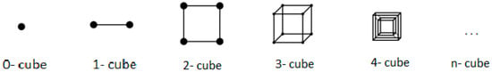
Figure 1. Progression of dimensional structures from 0-cube to n-cube.

This dimensional progression aims to provide an intuitive visualization that also helps understand how properties and operations scale with increasing system dimensionality. Properties that are evident in low dimensions (such as connectivity in a graph) can be generalized to higher dimensions, guiding the development of efficient algorithms for complex systems.

2.2.2. Topological Properties of the State Space

The geometric representation of the system as a hypercube induces a rich topological structure that determines the essential properties of the state space. These topological properties are not mere mathematical accessories; they constitute the foundation for developing algorithms for optimal bipartition identification. Moreover, this representation not only captures inherent topological properties but also significantly reduces computational complexity in extended combinatorial problems. Recent advancements in geometric intersection graphs, such as the approximation algorithms proposed Har-Peled and Yang [22], demonstrate the utility of efficient strategies for identifying maximal matchings, providing a robust framework for analyzing high-dimensional topologies.

Hamming Distance and Adjacency Structure. The Hamming distance between two binary states is defined as the number of positions in which their binary representations differ. In the hypercube context, this distance corresponds exactly to the minimum number of edges that must be traversed to go from one vertex to another.

Calculation and Interpretation of Hamming Distance. Formally, for two states x = (x₁, x₂, …, x_n) and y = (y₁, y₂, …, y_n) where xᵢ, yᵢ ∈ {0,1}, the Hamming distance is defined as (Equation (4))

$$d_H\left(x,y\right)={\sum }_{i=1}^n\left|x_i-y_i\right|={\sum }_{i=1}^n(x_i\oplus y_i)$$

(4)

where ⊕ denotes the XOR operation (exclusive disjunction).

This distance has a natural interpretation in terms of transitions between states: it represents the minimum number of variables that must change their value to transform one state into another. For example:

-

d_H(000,001) = 1 they only differ in the last position

-

d_H(001,010) = 2 they differ in the first and second positions

-

d_H(000,111) = 3 they differ in all positions

The adjacency structure of the hypercube is completely determined by the Hamming distance: two vertices are adjacent (connected by an edge) if and only if their Hamming distance is exactly 1. Figure 2 illustrates a 3-cube with Hamming distances d_H = 1 (blue, solid), d_H = 2 (red, dashed), and d_H = 3 (green, dotted).

Figure 2. Representation of a 3-cube with vertices labeled using binary coordinates.

Optimal Routes in State Space. The Hamming distance induces a natural metric in the state space, enabling the definition and calculation of optimal routes between states. An optimal route between two states corresponds to a minimum-length path in the hypercube, where each step involves changing the value of exactly one variable.

Dimensional Invariance and Geometric Transformations. The hypercube structure exhibits invariance properties under certain transformations, which allows identifying equivalences between apparently distinct system configurations.

Transformations that Preserve Structure. Among the transformations that preserve the topological structure of the hypercube are:

-

Coordinate permutations: Correspond to reordering system variables without altering their functional relationships.

-

Coordinate complementation: Equivalent to inverting the interpretation of a variable (swapping values 0 and 1).

-

Hypercube automorphisms: Transformations that preserve the adjacency structure, generated by combinations of the previous operations.

These transformations form the symmetry group of the hypercube, whose order is 2ⁿ·n! for an n-cube, reflecting the 2ⁿ possible coordinate inversions and the n! permutations of the n dimensions.

Implications for System Analysis. The dimensional invariance properties have profound implications for bipartition analysis:

• Search space reduction, many apparently distinct bipartitions are equivalent under structure-preserving transformations, enabling significant reduction in the number of configurations to evaluate.
• Identification of structural patterns, hypercube symmetries reveal structural patterns in system dynamics that can be exploited to identify optimal bipartitions.
• Result generalization, results obtained for certain subsystems can be generalized to other equivalent subsystems under appropriate transformations.

By exploiting these invariance properties, we can develop more efficient algorithms that selectively explore the solution space, focusing on canonical representatives of equivalence classes rather than evaluating each configuration individually.

The identification and exploitation of these topological properties constitute one of the fundamental pillars of our approach, enabling reduction in the inherent computational complexity of the optimal bipartition problem without sacrificing the quality of the solution found.

3. Methods

This section presents the methodological proposal based on geometric representation. Building from the established correspondence between the discrete system and n-dimensional space, we develop an approach that reformulates the optimal bipartition problem in terms of the topological structure of the hypercube and its intrinsic properties. The proposed methodology is grounded in two main pillars: (1) analysis of transitions between states through a topologically informed cost function, and (2) evaluation of candidate bipartitions using invariance properties and marginal distributions, avoiding the need to explicitly reconstruct the complete system.

3.1. Geometric Reformulation

Having established the correspondence between the discrete system and the n-dimensional geometric space, we now proceed to reformulate the optimal bipartition problem by leveraging this spatial interpretation. The geometric reformulation not only provides a new conceptual perspective but also establishes the foundations for a more efficient algorithmic approach.

The traditional problem of finding an optimal system bipartition transforms into a topological analysis problem of the associated hypercube, where we seek to identify a division that optimally preserves certain structural properties. This transformation enables us to exploit intrinsic characteristics of the state space that are not evident in the original formulation.

3.1.1. Cost Function for Transitions Between States

A fundamental component is the definition of a cost function t(i, j) that quantifies the “inertia” or “energy” required for the transition between two states i, j of the system. This function captures the underlying causal structure of the system and provides the foundation for identifying natural bipartitions. It is worth highlighting that our geometric approach conceptual alignment with IIT 4.0’s emphasis on causal structure and “cause-effect powers” as the foundation of consciousness [7] while building upon IIT 3.0 mathematical foundations. The hypercube topology provides a natural framework for analyzing causal irreducibility: (a) Hamming Distance as Causal Influence Metric: The Hamming distance between hypercube vertices directly reflects the causal influence magnitude between system parts. States at distance 1 represent minimal causal interventions (single variable changes), while greater distances correspond to increasingly complex causal interactions. This geometric mapping enables quantitative analysis of how causal structure emerges from system topology. (b) Topological Irreducibility: The geometric cost function t(i,j) captures causal irreducibility by quantifying the “energy” required for causal transitions. Optimal bipartitions correspond to natural causal boundaries where the system resists decomposition—precisely the irreducibility criterion emphasized in IIT 4.0. The exponential decay factor γ = 2^(−dH(i,j)) mathematically encodes how causal influence diminishes with topological distance, providing a geometric foundation for consciousness quantification. (c) Cause-Effect Power Representation: The hypercube structure enables direct visualization and computation of cause-effect relationships through transition pathways. Each edge represents an elementary causal transformation, while paths between distant vertices capture complex causal chains. This topological representation makes explicit the causal structure that IIT 4.0 identifies as fundamental to conscious experience.

Building on this causal foundation, unlike traditional metrics that consider only direct transitions between states, t(i,j) integrates the concept of topological distance in the hypercube, recognizing that transitions between distant states imply multiple intermediate elementary transformations.

Formally, the cost function t: V × V → ℝ is defined for the transition between states i, j as (Equation (5)):

$$t_x(i,j) = \gamma ·\left(\left|X\left[i\right]- X\left[j\right]\right|\right)+ {\sum }_{kϵN(i,j)}\left\{t_x\left(k,j\right)\right\}$$

(5)

where

γ = 2^(−dH(i,j)) is an exponential decay factor based on the Hamming distance between states i and j

d_H(i, j) is the Hamming distance between states i and j.

X[i] represents the value associated with state i (conditional probability).

N(i,j) denotes the immediate sub-neighbors of i that are on some optimal path to j.

The resulting table T from applying this function to all pairs of states constitutes a complete map of causal relationships in the system, revealing structural patterns that will guide the identification of optimal bipartitions.

Connection to the Bipartition Problem: The cost function t(i,j) defined in Equation (5) serves as the computational foundation for solving the optimal bipartition problem formulated in Equation (1). This connection operates through several key mathematical relationships:

(1)

Direct relationship to EMD computation: The EMD d in Equation (1) measures the discrepancy between original system dynamics P(V_t+1|V_t) and reconstructed dynamics from bipartitions. The cost function t(i,j) provides the transition costs that EMD uses to compute this discrepancy—specifically, EMD calculates the minimum cost to transform one probability distribution into another, where these costs are precisely the values t(i,j) computed through Equation (5).

(2)

Bipartition evaluation mechanism: For any candidate bipartition {S₁, S₂}, the discrepancy δ(V,{S₁,S₂}) in Equation (1) is computed by applying EMD with the cost matrix T derived from Equation (5). The geometric approach leverages the fact that optimal bipartitions correspond to divisions where the cumulative transition costs (captured in table T) reveal natural boundaries in the system’s causal structure.

(3)

Computational advantage: Rather than exhaustively evaluating all possible bipartitions through direct EMD computation (which would require O(2ⁿ) operations), our methodology uses the structural patterns in cost table T to directly identify candidate bipartitions that minimize the objective function in Equation (1). The geometric analysis of transition costs reveals complementarity patterns that correspond to minimal discrepancy bipartitions, enabling direct identification of solutions to the optimization problem without exhaustive search.

This mathematical bridge ensures that bipartitions identified through geometric analysis of table T correspond precisely to those that minimize the information-theoretic discrepancy δ defined in the original bipartition problem.

Exponential Decay Factors. A critical aspect of the cost function t(i, j) is the exponential decay factor γ = 2^(−dH(i,j)) which determines how the influence of differences between states diminishes with topological distance. The choice of an exponential decay factor, rather than other functions such as linear or logarithmic, is based on both theoretical and practical considerations: Regarding theoretical considerations, we know, for example, that in causal systems, the influence of one event on another typically decays exponentially with the “distance” (temporal, spatial, or topological) between them. This behavior is observed in physical, biological, and social phenomena. In terms of mathematical properties, the exponential function 2^(−d) possesses convenient algebraic properties, such as the fact that 2^(−(d₁^+d₂⁾⁾ = 2^(−d₁⁾·2^(−d₂⁾, which allows decomposing complex transitions into elementary components and enables efficient recursive exploration of state space through elementary component analysis. Likewise, it presents a correlation with EMD calculation rooted in its nature. The base-2 selection specifically aligns with binary hypercube transitions, where each distance increment represents a fundamental bit-flip operation. Finally, asymptotic behavior is very important because with this function, the influence never reaches exactly zero but becomes arbitrarily small for large distances, reflecting the principle that everything can influence everything, but with very different practical magnitudes mathematically embodying the principle that distant relationships maintain theoretical significance while practical impact diminishes appropriately. Figure 3 shows the comparison of the exponential decay factor γ = 2^(−d) with other types of decay as a function of distance d. The exponential decay adequately captures the dilution of causal influence with topological distance.

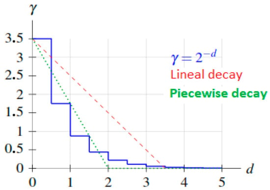
Figure 3. Exponential decay factor.

On the other hand, the exponential factor has significant effects on the analysis of transitions between states:

-

Natural path weighting: When calculating t(i, j) through recursive exploration of the hypercube, shorter paths automatically receive greater weight in the total contribution.

-

Effect localization: Differences between nearby states dominate the calculation, reflecting the intuition that local interactions are generally stronger than distant ones.

This exponential weighting has a particularly important effect in high-dimensional systems, where the number of states and possible transitions grows exponentially, but only a subset of these relationships proves significant for the causal structure of the system.

Comparative Analysis and Optimization: Our foundational analysis evaluated linear and logarithmic decay alternatives, revealing critical limitations that support the exponential choice. Linear decay functions fail to capture the rapid diminishment of causal influence characteristic of complex systems, resulting in distant state relationships contributing disproportionate weight to partition decisions. This leads to suboptimal bipartition identification that overemphasizes peripheral system interactions. Logarithmic decay functions reduce distant state influence too aggressively, creating cost functions insufficiently sensitive to important multi-step causal relationships. The exponential formulation provides optimal balance, maintaining sensitivity to meaningful causal relationships across multiple Hamming distance levels while ensuring partition decisions remain anchored in the most relevant system interactions.

Empirical Validation and Robust Performance: Extensive validation across multiple system configurations demonstrated consistent performance characteristics with the exponential formulation. The factor produces stable partition identification across systems of varying complexity and structure, indicating robust mathematical behavior that translates effectively to diverse computational scenarios. Particularly in systems with 3–15 variables, where the balance between local and global causal relationship preservation is critical, the exponential decay has proven superior to alternatives. The validation encompassed diverse system topologies, ranging from weakly connected networks to highly integrated structures, consistently demonstrating that the exponential approach identifies partitions that minimize information-theoretic discrepancy while maintaining computational tractability.

The exponential weighting produces several critical optimization effects: natural path weighting during recursive exploration automatically prioritizes shorter paths in contribution calculations, effect localization ensures nearby states dominate cost computations while preserving sensitivity to relevant long-range dependencies, and high-dimensional system optimization prevents computational explosion from irrelevant state interactions. These effects combine to create a cost function that scales effectively with system complexity while maintaining theoretical rigor in partition identification.

Recursive Exploration of State Space. The calculation of the cost function t(i, j) for all pairs of states requires systematic exploration of the hypercube. Since the number of states grows exponentially with system dimensionality, it is crucial to implement an efficient algorithm for this exploration. A modified Breadth-First Search (BFS) algorithm is proposed that explores the hypercube level by level, accumulating contributions to the cost with appropriate weighting (see Algorithm 1). This algorithm constructs the complete cost table T, capturing the causal structure of the system represented in the hypercube. The resulting table serves as the foundation for identification and evaluation of potential bipartitions.

Optimizations for Large-Scale Systems. For large-scale systems, where dimensionality may make exhaustive calculation prohibitive, optimizations can be proposed such as:

-

Parallelization: The calculation of t(i, j) for different pairs (i, j) is inherently parallelizable, enabling efficient implementation in multicore or distributed architectures.

-

Sampling-based approximation: For extremely large systems, use sampling techniques to estimate t(i, j) values instead of calculating them exactly for all pairs.

-

Leveraging symmetries: Utilize the symmetry properties of the hypercube to reduce the number of necessary calculations, recognizing that many pairs of states are equivalent under structure-preserving transformations.

These optimizations enable extending the applicability of our methodology to systems with tens or even hundreds of variables, where traditional approaches would be completely infeasible.

Algorithm 1. Calculation of Cost Table T using BFS modified

1: Input: Hipercubo G = (V, E), values X [v] for each vertex v ∈ V

2: Output: Cost Table T, T [i, j] = t (i, j) for all i, j ∈V

3: for each pair of vertices(i, j) ∈ V × V do

4:     T [i, j] ← 0

5:     d ← dH (i, j)

6:     γ ← 2−d

7:     T [i, j] ← |X [i] − X [j]|

8:     if d > 1 then

9:        Q ← {i}

10:        visited ← {i}

11:        level ← 0

12:        while level < d and Q not empty do

13:           level ← level + 1

14:           next Q ← {}

15:           for each vertex u ∈ Q do

16:              for each neighbor v of u such that dH (v, j) < dH (u, j) do

17:                   if v ∉ visited then

18:                       T [i, j] ← γ (T [i, j] + T [i, v])

19:                       visited ← visited ∪ {v}

20:                       next Q ← next Q ∪ {v}

21:                   end if

22:              end for

23:               end for

24:               Q ← next Q

25:        end while

26:     end if

27: end for

28: return T

3.1.2. Bipartition Evaluation via Tensorial Discrepancy

Once the cost table T is calculated, we proceed to use it for evaluating the quality of possible system bipartitions. Unlike traditional approaches that require reconstructing the complete system through tensor products, our methodology leverages geometric properties and marginal distributions for more direct and efficient evaluation.

Marginal distributions and geometric projections. A key concept in our methodology is the use of marginal distributions as geometric projections in n-dimensional space. This approach eliminates the need to explicitly reconstruct the system through tensor products, significantly reducing computational complexity. Figure 4 shows the Visualization of marginal distributions as geometric projections in a three-variable system. Projections on different planes correspond to marginalizing over distinct subsets of variables.

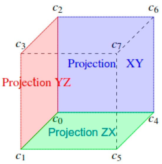
Figure 4. Visualization of marginal distributions as geometric projections.

When we consider a bipartition S = {S₁, S₂} of the system, each part Sᵢ defines a subspace in the n-dimensional hypercube. The properties of these subspaces and their interrelationships determine the quality of the bipartition.

The traditional methodology would evaluate the discrepancy between the original system dynamics and the dynamics reconstructed through the tensor product of the parts. In contrast, our approach exploits the fact that this discrepancy can be characterized directly through geometric properties of the hypercube and the associated marginal distributions.

-

Dimensional projection: A marginal distribution corresponds geometrically to a projection of the hypercube onto a lower-dimensional subspace.

-

Information preservation: The projection preserves certain information about the original structure but inevitably loses some relationships when reducing dimensionality.

-

Structural independence: Two subsets of variables are functionally independent if their corresponding projections capture all relevant information from the original system.

The functional independence between variable subsets manifests geometrically as a decomposition property of the hypercube, where projections onto complementary subspaces are sufficient to completely characterize the system.

The core algorithm representing the mathematical model expressed in Equation (5) is presented below (see Algorithm 2).

Algorithm 2. Geometric Algorithm

1: Input: Subsystem S with n variables

2: Output: Optimal Bipartition Bopt

3: tensors ← DescomposeIntoTensors(S)

4: T ← InitializeTransitionTable()

5: for each variable v en S do

6:    for each initial state i do

7:       for each final state j do

8:           T [v, i, j] ← CalculateTransitionTableCost(i, j, tensors[v])

9:        end for

10:   end for

11: end for

12: candidates ← IdentifyCandidateBipartitions(T)

13: Bopt ← EvaluateCandidates(candidates, S, T)

14: return Bopt

3.2. Test Data

The evaluation of the Geometric Strategy was conducted using a carefully designed dataset comprising both synthetic and real-world data. This diverse dataset aimed to validate the strategy’s efficacy and scalability while ensuring compatibility with established standards in Integrated Information Theory (IIT).The test suite used to evaluate the strategies employs both synthetic data, which are fundamental elements in research and are generated by simulations or computational models [14], as well as real-world data taken from previous research studies that allowed us to construct the final dataset for our tests.

Key scenarios included (see Table 2):

Table 2. Datasets and network sizes used in the testing process.

	Network Size	Number of Subsystems
Synthetic Data	3 nodes	25
Synthetic Data	4 nodes	50
Synthetic Data	5 nodes	50
Synthetic Data	6 nodes	50
Synthetic Data	10 nodes	50
Synthetic Data	20 nodes	50
Synthetic Data	21 nodes	50
Synthetic Data	22 nodes	50
Real Data	15 nodes (Network A)	50
Real Data	15 nodes (Network B)	50

-

Network Sizes: The networks covered a spectrum from small systems of 3 nodes to larger configurations of up to 22 nodes. These sizes reflect the range in which IIT computations remain computationally feasible.

-

Subsystem Analysis: Each network involved analyzing up to 50 subsystems, with each configuration designed to explore conditional relationships across nodes at time t and t + 1.

-

Evaluation Variables: Parameters like transition probability matrices (TPMs) and the ground truth bipartitions were crucial for benchmarking accuracy.

A subsystem is defined as the conditional relationship between the states of the nodes at time $t+1$ given their configuration at time $t$, mathematically represented as a conditional probability $P(elements at t+1 | elements at t)$. For each network, various configurations of nodes in the states $t$ and $t+1$ were explored, evaluating their influence on the dynamics of the system and the structure of the resulting partitions.

For each test system, both the transition matrix (TPM) and the expected optimal bipartition, were calculated using PyPhi’s exhaustive algorithm.

3.2.1. Synthetic Data

The synthetic datasets were generated from probabilistic models grounded in the IIT framework. Specifically, the synthetic networks were derived from the official IIT documentation is used (Multiple networks provided in IIT 3.0 Paper (2014) were used—v1.2.0 documentation, https://pyphi.readthedocs.io/en/latest/examples/2014paper.html (accessed on 5 August 2025)), expanding beyond the basic templates provided. This ensured the representation of a wide range of causal dynamics and system complexities. It is also possible to generate data for systems of user-specified sizes in order to generate networks large enough to assess the scope of the strategy.

3.2.2. Real-World Data

Complementing the synthetic data, real-world datasets enhanced the ecological validity of the experiments. These datasets, derived from previous studies [23,24], included neural activity models from Drosophila melanogaster. The TPMs generated by these studies provided insights into dynamic systems analogous to those observed in biological networks. These investigations provided the base methodology for building the integrated information structure (IIS) from local field potentials (LFPs) [25] and offered detailed descriptions of the LFP data and the preprocessing steps. Based on this information, we built the final dataset for testing our strategy, so that a TPM is generated for each fly in a specific state (awake or under anesthesia) and for the entire period. This means that for each fly there are two TPMs, one for each specific state (awake or under anesthesia). For 13 flies in the study, there is a total of 26 TPMs. However, in our tests, we worked with two TPMs corresponding to a randomly selected fly, as we observed similar results across all 13 flies after review.

Highlights of real-world data:

-

Empirical Basis: The networks modeled actual biological systems and were crucial for validating the scalability and applicability of the geometric approach.

-

Network Structures: These datasets encompassed networks with up to 15 nodes, fully exploring all possible states and transitions within these configurations.

3.2.3. Analytical Framework

To quantitatively assess the performance, the datasets were designed to address multiple dimensions:

-

System Size: Simulations scaled from small (3 nodes) to moderately large systems (22 nodes).

-

Causality Analysis: Various configurations of input-output relationships were tested, examining how causal structures influence system dynamics.

-

Ground Truth Validation: For networks within PyPhi’s computational limits, the optimal bipartitions were precomputed using PyPhi’s exhaustive algorithm, serving as the reference for accuracy validation.

3.3. Evaluation Metrics

The evaluation of the implementations will be based on two fundamental aspects: the correctness of results (accuracy) and computational performance (efficiency). The quantitative evaluation of the implementation will be based on the following metrics.

3.3.1. Error and Precision Analysis

Since the geometric approach may not always guarantee the optimal bipartition (especially in complex systems), it is crucial to quantify the quality of the solutions found:

-

Hit Rate (Agreement rate): Percentage of cases where the bipartition found coincides exactly with the optimal one (according to PyPhi).

-

Relative error in $\phi$: For cases where the bipartition differs, calculate as (Equation (6)):

$$E_{rel}={\displaystyle \frac{\left|{\phi }_{optimal}-{\phi }_{found}\right|}{{\phi }_{optimal}}}$$

(6)

Structural distance: The maximum structural distance refers to the partition that showed the least similarity between the one identified by strategy X and the one identified by the new strategy. For this metric, the Jaccard distance was used, which is calculated as follows (Equation (7)):

$$d_j\left(X,Y\right)=1-{\displaystyle \frac{\left|X\cap Y\right|}{\left|X\cup Y\right|}}$$

(7)

Speedup: The relative speedup refers to the average acceleration of the execution times of the strategy compared to strategy X. It was calculated as follows (Equation (8)):

$$S_{rel}={\displaystyle \frac{T_{Strategy X}}{T_{Geometric}}}$$

(8)

Below, we show in Table 3 establishes the acceptability thresholds for these metrics.

Table 3. Acceptability thresholds for error and precision metrics.

Quality Level	Agreement Rate	Max. Relative Error	Max. Structural Distance
Excellent	>90%	<1%	<0.1
Good	>80%	<5%	<0.2
Acceptable	>70%	<10%	<0.3
Insufficient	<70%	>10%	>0.3

3.3.2. Temporal Performance Comparison

Computational performance will be evaluated through:

Relative speedup: Acceleration factor relative to PyPhi, calculated as presented in the following expression (Equation (9)):

$$S_{rel}={\displaystyle \frac{T_{PyPhi}}{T_{Geometric}}}$$

(9)

-

Scalability: Relationship between execution time and system size, comparing observed asymptotic behavior with theoretical behavior.

-

Memory usage: Maximum memory consumption during algorithm execution.

3.4. Cross-Validation Strategies

The validation of the implementation followed these stages:

-

Small case validation: Verify correctness in small systems (3–5 variables) where the optimal result is known and can be verified manually against brute force.

-

Comparison with PyPhi: For medium-sized systems (6–10 variables), compare results with those obtained by PyPhi, which implements the exhaustive algorithm and guarantees optimal results.

-

Scalability: For large systems (>20 variables), where PyPhi becomes computationally intractable, we use QNodes as our reference implementation. QNodes is our own research development, currently under peer review, which provides a theoretically sound and empirically validated approach for MIP identification in large-scale systems.

-

Technical Foundation of QNodes:

○

Submodularity Discovery: Our research demonstrated that the EMD, loss function, is submodular in the IIT context, enabling the application of polynomial-time optimization algorithms.

○

Queyranne’s Algorithm Implementation: Leverages Queyranne’s algorithm for symmetric submodular function minimization, achieving O(N³) complexity versus the exponential O(2^N) of exhaustive approaches.

○

N-Cube Representation: Employs multidimensional N-cube data structures for efficient manipulation of conditional probability distributions, dramatically reducing computational overhead.

○

Perfect Accuracy Validation: Achieved 100% agreement with PyPhi across all network sizes (3–20 nodes) where direct comparison was possible, confirming theoretical predictions.

-

Rationale for QNodes Selection:

○

Theoretical Rigor: Unlike heuristic methods, QNodes provides mathematically guaranteed optimal solutions through submodular optimization.

○

Proven Scalability: Successfully processes systems up to 22 variables where PyPhi fails due to computational constraints.

○

Empirical Validation: Extensive benchmarking against PyPhi ground truth demonstrates perfect MIP identification accuracy.

○

Algorithmic Transparency: Complete knowledge of implementation details enables precise interpretation of performance comparisons.

-

Performance Characteristics: QNodes achieves exponential speedups (8.32× to 1531× vs. traditional methods) while maintaining perfect accuracy, making it the most suitable reference for evaluating our geometric approach in large-scale systems where exhaustive methods become computationally prohibitive.

3.5. Experimental Methodology

The experimental validation follows a comprehensive methodology designed to evaluate both accuracy and computational efficiency across diverse system scales. The evaluation encompasses systems ranging from 3 to 22 nodes, with PyPhi serving as the ground truth reference for smaller systems and QNodes implementations providing benchmarks for larger systems where PyPhi becomes computationally infeasible. The experimental protocol involves multiple test runs for each system configuration to ensure statistical reliability and account for computational variance.

The evaluation metrics provide comprehensive coverage of algorithm performance characteristics, including (a) exact match hit rates for bipartition identification, (b) relative error measurements for ϕ value accuracy, this error ϕ represents the discrepancy between Φ values computed by GeoMIP versus reference implementations (PyPhi/QNodes), since in IIT, Φ corresponds directly to the loss value calculated through EMD between original and reconstructed system dynamics, (c) structural distance analysis using EMD metrics, and execution time comparisons for speedup calculations. For the 20-node systems, the methodology includes comparison against QNodes implementation, providing insights into the relative performance of different optimization strategies. The experimental results are systematically recorded and analyzed using tools like Excel spreadsheets, ensuring reproducibility and facilitating detailed performance analysis across different system configurations and algorithm parameters.

4. Results and Discussion

After developing the theoretical and methodological framework for the geometric representation of the optimal bipartition problem, we now proceed to apply these concepts to a concrete case. This section presents a detailed analysis of a simple three-variable subsystem, illustrating step by step how our methodology enables identification of optimal bipartitions.

4.1. Analysis of a Three-Variable Subsystem

Consider a subsystem composed of three binary variables V = {A, B, C}. This subsystem will allow us to illustrate the principles and enable clear visualization of the underlying concepts.

4.1.1. Construction of the Geometric Space

Modeling of the Original Subsystem

Our example subsystem consists of three binary variables (which can take values 0 or 1). The subsystem dynamics are defined by a transition probability matrix (TPM) (This dataset can be found in GitHub repository as the 3-Node Network C, “N3C.csv”) that specifies the probability of each possible state at time t + 1 given each possible state at time t.

For a three-variable subsystem, the complete TPM in state-to-state format would be an 8 × 8 matrix, where rows represent the 2³ = 8 possible states at time t and columns represent states at time t + 1. However, for our analysis based on geometric representation, we will work with the decomposed state-to-node form, where each future variable is represented separately (it would contain dimensions of 8 × 3 as previously tabulated).

Representation as Hypercube. The geometric representation of the subsystem corresponds to a three-dimensional hypercube (cube), where each vertex represents one of the 2^|Vs|=3 = 8 possible states of the subsystem, labeled according to their binary representation with the dataset in its OFF state.

Table 4 presents the representation of the TPM in state-to-node form. Figure 5 shows the representation of the three-variable subsystem as a three-dimensional cube. Each vertex corresponds to a possible state of the subsystem, labeled according to its binary representation.

Table 4. TPM representation state by node.

		At+1 (OOF)	Bt+1 (OOF)	Ct+1 (OOF)
Abct	000	0	0	0
	100	0	0	1
	010	0	1	0
	110	0	1	1
	001	1	0	0
	101	1	0	1
	011	1	1	0
	111	1	1	1

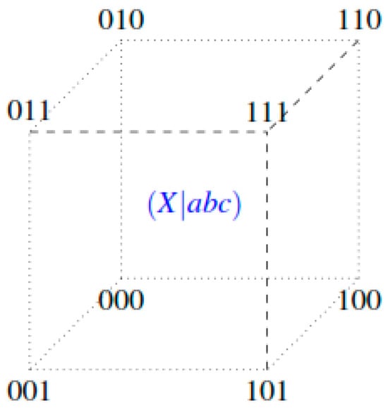
Figure 5. Representation of the three-variable subsystem as a three-dimensional cube.

In this representation:

-

The first digit corresponds to the value of variable/dimension a.

-

The second digit corresponds to the value of variable/dimension b.

-

The third digit corresponds to the value of variable/dimension c.

The geometric structure of the cube naturally captures the adjacency relationship between states: two states are adjacent (connected by an edge) if and only if they differ in exactly one variable. This property will be fundamental for our analysis of transitions between states.

4.1.2. Decomposition into Elementary Tensors

Following the principle of conditional independence, we can decompose the subsystem dynamics into three elementary tensors, each representing the conditional probability of a specific variable at time t + 1 given the complete state of the subsystem at time t.

-

Individual Tensors for Each Variable. For our example subsystem, consider the following values for the elementary tensors, which represent P(A_t+1|abc_t), P(B_t+1|abc_t), and P(C_t+1|abc_t) respectively. This structure illustrates a subsystem with specific causal dependencies between variables at different times.

-

Verification of the Decomposition. The tensorial decomposition allows us to reconstruct the complete dynamics of the subsystem through the tensor product of elementary tensors. For each initial state abc_t, we can determine the probability distribution over states ABC_t+1 by combining the conditional probabilities of each individual variable.

Figure 6 presents the decomposition of the subsystem into three n-cubes (tensors) representing the conditional probabilities of each future variable. The values associated with each vertex represent the probability that the corresponding variable takes the value 0 at t + 1 given the specific state of the subsystem at time t.

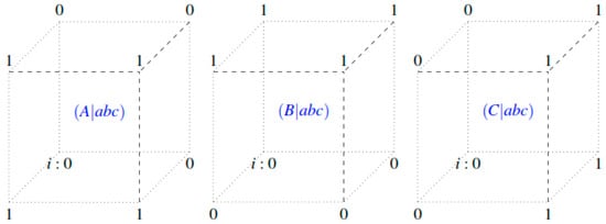
Figure 6. Decomposition of the subsystem into three n-cubes (tensors).

For example, for the initial state abc_t = 000:

P(A_t+1 = 0|abc_t = 000) = 0 (tensor A)

P(B_t+1 = 0|abc_t = 000) = 0 (tensor B)

P(C_t+1 = 0|abc_t = 000) = 0 (tensor C)

This implies that P(ABC_t+1 = 000|abc_t = 000) = 0·0·0 = 0, meaning the subsystem remains in state 000 with probability 0.

4.2. Cost Function Calculation and Space Exploration

Having established the geometric representation and tensorial decomposition of the subsystem, we now proceed to apply the cost function t(i, j) to analyze transitions between states and construct table T that will guide the identification of optimal bipartitions.

4.2.1. Transition Example State 000 to State 011

To illustrate the cost function calculation process, we will analyze in detail the transition from initial state i = 000 to state j = 011.

For the analysis of possible paths, we have that the Hamming distance between i = 000 and j = 011 is d_H(000,011) = 2, meaning they differ in exactly two positions (the second and third). There exist two possible optimal paths between these states

000 → 010 → 011 (changing B first, then C)

000 → 001 → 011 (changing C first, then B)

Each of these paths has length 2 (minimum possible), but they may have different associated costs depending on the conditional probabilities in the intermediate states.

4.2.2. Systematic Construction of the Cost Table

Starting from initial state i = 000, we apply the cost function t(i, j) to calculate the transition cost to all possible states j. This process can follow a bottom-up strategy, first calculating costs for adjacent states (Hamming distance = 1), then for states at distance 2, and finally for the most distant state (distance 3). Figure 7 shows the visualization of the two possible “optimal” paths from state 000 to state 011. The blue path passes through 010, while the red path passes through 001.

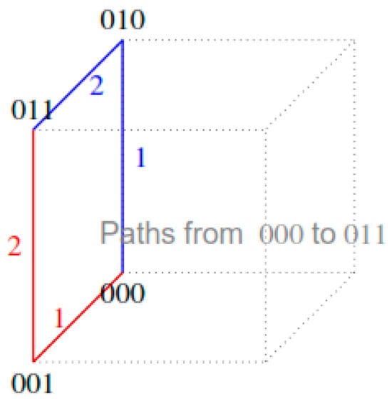
Figure 7. Visualization of the possible optimal paths from state 000 to state 011.

The cost function t(i, j) is defined as previously mentioned (Equation (5)):

$$t_x(i,j) = \gamma ·(\left|X\left[i\right]- X\left[j\right]\right|+ \sum _{kϵN(i,j)}{t}_x\left(k,j\right))$$

Calculations for Variable A: We proceed to systematically calculate the transition costs from initial state 000 to all other states for variable A:

For states at Hamming distance = 1:

$$t_A\left(\mathrm{000,100}\right)= 2^{-1}.(\left|A\left[000\right]-A\left[100\right]\right|+0)$$

$$={\displaystyle \frac{1}{2}} .\left(\left|0-0\right|+0\right)=0$$

$$t_A\left(\mathrm{000,010}\right)=2^{-1}.(\left|A\left[000\right]-A\left[010\right]\right|+0)$$

$$={\displaystyle \frac{1}{2}} .\left(\left|0-0\right|+0\right)=0$$

$$t_A\left(\mathrm{000,001}\right)=2^{-1}.(\left|A\left[000\right]-A\left[001\right]\right|+0)$$

$$={\displaystyle \frac{1}{2}} .\left(\left|0-1\right|+0\right)={\displaystyle \frac{1}{2}}$$

For states at Hamming distance = 2:

$$t_A\left(\mathrm{000,110}\right)= 2^{-2}.(\left|A\left[000\right]-A\left[110\right]\right|+t_A\left(\mathrm{000,100}\right)+t_A\left(\mathrm{000,010}\right))$$

$$={\displaystyle \frac{1}{4}} .\left(\left|0-0\right|+0+0\right)=0$$

$$t_A\left(\mathrm{000,101}\right)=2^{-2}.(\left|A\left[000\right]-A\left[101\right]\right|+t_A\left(\mathrm{000,100}\right)+t_A\left(\mathrm{000,001}\right))$$

$$={\displaystyle \frac{1}{4}} .\left(\left|0-1\right|+0+{\displaystyle \frac{1}{2}}\right)={\displaystyle \frac{3}{8}}$$

$$t_A\left(\mathrm{000,011}\right)=2^{-2}.(\left|A\left[000\right]-A\left[011\right]\right|+t_A\left(\mathrm{000,010}\right)+t_A\left(\mathrm{000,001}\right))$$

$$={\displaystyle \frac{1}{4}} .\left(\left|0-1\right|+0+{\displaystyle \frac{1}{2}}\right)={\displaystyle \frac{3}{8}}$$

For states at Hamming distance = 3:

$$t_A\left(\mathrm{000,111}\right)= 2^{-3}.\left(\left|A\left[000\right]-A\left[111\right]\right|+t_A\left(\mathrm{000,110}\right)+t_A\left(\mathrm{000,101}\right)\right)+t_A\left(\mathrm{000,011}\right)$$

$$={\displaystyle \frac{1}{8}} .\left(\left|0-1\right|+0+{\displaystyle \frac{3}{8}}+{\displaystyle \frac{3}{8}}\right)={\displaystyle \frac{14}{8}}$$

Calculations for Variable B: We perform the same calculations for variable B:

For states at Hamming distance = 1:

$$t_B\left(\mathrm{000,100}\right)= 2^{-1}.(\left|B\left[000\right]-B\left[100\right]\right|+0)$$

$$={\displaystyle \frac{1}{2}} .\left(\left|0-0\right|+0\right)=0$$

$$t_B\left(\mathrm{000,010}\right)=2^{-1}.(\left|B\left[000\right]-B\left[010\right]\right|+0)$$

$$={\displaystyle \frac{1}{2}} .\left(\left|0-1\right|+0\right)={\displaystyle \frac{1}{2}}$$

$$t_B\left(\mathrm{000,001}\right)=2^{-1}.(\left|B\left[000\right]-B\left[001\right]\right|+0)$$

$$={\displaystyle \frac{1}{2}} .\left(\left|0-0\right|+0\right)=0$$

For states at Hamming distance = 2:

$$t_B\left(\mathrm{000,110}\right)= 2^{-2}.(\left|B\left[000\right]-B\left[110\right]\right|+t_B\left(\mathrm{000,100}\right)+t_B\left(\mathrm{000,010}\right))$$

$$={\displaystyle \frac{1}{4}} .\left(\left|0-1\right|+0+{\displaystyle \frac{1}{2}}\right)={\displaystyle \frac{3}{8}}$$

$$t_B\left(\mathrm{000,101}\right)=2^{-2}.(\left|B\left[000\right]-B\left[101\right]\right|+t_B\left(\mathrm{000,100}\right)+t_B\left(\mathrm{000,001}\right))$$

$$={\displaystyle \frac{1}{4}} .\left(\left|0-0\right|+0+0\right)=0$$

$$t_B\left(\mathrm{000,011}\right)=2^{-2}.(\left|B\left[000\right]-B\left[011\right]\right|+t_B\left(\mathrm{000,010}\right)+t_B\left(\mathrm{000,001}\right))$$

$$={\displaystyle \frac{1}{4}} .\left(\left|0-1\right|+{\displaystyle \frac{1}{2}}+0\right)={\displaystyle \frac{3}{8}}$$

For states at Hamming distance = 3:

$$t_B\left(\mathrm{000,111}\right)= 2^{-3}.(\left|B\left[000\right]-B\left[111\right]\right|+t_B\left(\mathrm{000,110}\right)+t_B\left(\mathrm{000,101}\right)+t_B\left(\mathrm{000,011}\right))$$

$$={\displaystyle \frac{1}{8}} .\left(\left|0-1\right|+{\displaystyle \frac{3}{8}}+0+{\displaystyle \frac{3}{8}}\right)={\displaystyle \frac{7}{32}}$$

Calculations for Variable C: Finally, we perform the calculations for variable C:

For states at Hamming distance = 1:

$$t_C\left(\mathrm{000,100}\right)= 2^{-1}.(\left|C\left[000\right]-C\left[100\right]\right|+0)$$

$$={\displaystyle \frac{1}{2}} .\left(\left|0-1\right|+0\right)={\displaystyle \frac{1}{2}}$$

$$t_C\left(\mathrm{000,100}\right)=2^{-1}.(\left|C\left[000\right]-C\left[010\right]\right|+0)$$

$$={\displaystyle \frac{1}{2}} .\left(\left|0-0\right|+0\right)=0$$

$$t_C\left(\mathrm{000,001}\right)=2^{-1}.(\left|C\left[000\right]-C\left[001\right]\right|+0)$$

$$={\displaystyle \frac{1}{2}} .\left(\left|0-0\right|+0\right)=0$$

For states at Hamming distance = 2:

$$t_C\left(\mathrm{000,110}\right)= 2^{-2}.(\left|C\left[000\right]-C\left[110\right]\right|+t_C\left(\mathrm{000,100}\right)+t_C\left(\mathrm{000,010}\right))$$

$$={\displaystyle \frac{1}{4}} .\left(\left|0-1\right|+{\displaystyle \frac{1}{2}}+0\right)={\displaystyle \frac{3}{8}}$$

$$t_C\left(\mathrm{000,101}\right)=2^{-2}.(\left|C\left[000\right]-C\left[101\right]\right|+t_C\left(\mathrm{000,100}\right)+t_C\left(\mathrm{000,001}\right))$$

$$={\displaystyle \frac{1}{4}} .\left(\left|0-1\right|+{\displaystyle \frac{1}{2}}+0\right)={\displaystyle \frac{3}{8}}$$

$$t_C\left(\mathrm{000,011}\right)=2^{-2}.(\left|C\left[000\right]-C\left[011\right]\right|+t_C\left(\mathrm{000,010}\right)+t_C\left(\mathrm{000,001}\right))$$

$$={\displaystyle \frac{1}{4}} .\left(\left|0-0\right|+0+0\right)=0$$

For states at Hamming distance = 3:

$$t_C\left(\mathrm{000,111}\right)= 2^{-3}.(\left|C\left[000\right]-C\left[111\right]\right|+t_C\left(\mathrm{000,110}\right)+t_C\left(\mathrm{000,101}\right)+t_C\left(\mathrm{000,011}\right))$$

$$={\displaystyle \frac{1}{8}} .\left(\left|0-1\right|+{\displaystyle \frac{3}{8}}+{\displaystyle \frac{3}{8}}+0\right)={\displaystyle \frac{7}{32}}$$

4.2.3. Complete Cost Table Results

Table 5 shows the calculated costs for all possible transitions from initial state 000 for each system variable:

Table 5. Transition costs from state 000 for each variable.

Transition	Variable A	Variable B	Variable C
t (000, 000)	0	0	0
t (000, 100)	0	0	0.5
t (000, 010)	0	0.5	0
t (000, 110)	0	0.375	0.375
t (000, 001)	0.5	0	0
t (000, 101)	0.375	0	0.375
t (000, 011)	0.375	0.375	0
t (000, 111)	0.219	0.279	0.219

Table 6 presents the execution of bipartitions using brute force to perform an initial validation of the results.

Table 6. Execution of bipartitions using brute force.

	000	001	010	011
000		0.50	0.50	1
001	0.50	1	1	1.50
010	0.50	1	0	0.50
011	1	1.50	0.50	1
100	0.50	0	1	0.50
101	1	0.50	1.50	1
110	1	0.50	0.50	0
111	1.50	1	1	0.50

4.2.4. Identification of Optimal Bipartitions

Analyzing the transition table T, we can identify complementarity patterns that reveal optimal bipartitions. An optimal bipartition is characterized by having complementary transition costs that minimize the total discrepancy.

Mathematical foundation: This analysis directly implements the optimization objective defined in Equation (1), where we seek bipartitions {S₁, S₂} that minimize δ(V,{S₁,S₂}). The complementarity patterns in table T correspond precisely to bipartitions where the Earth Mover’s Distance between original and reconstructed dynamics is minimized, as the EMD computation utilizes the transition costs t(i,j) from Equation (5) to measure the discrepancy between probability distributions.

From the cost table, we identify the minimum bipartitions (see Table 7) through complementarity analysis.

Table 7. Bipartitions identified through complementarity analysis.

Bipartition	Transitions A	Transitions B	Transitions C
First	A(000, 100) = 0	B(000, 100) = 0	C(000, 011) = 0
Second	A(000, 010) = 0	B(000, 101) = 0	C(000, 010) = 0
Third	A(000, 110) = 0	B(000, 001) = 0	C(000, 001) = 0

These bipartitions represent “natural” divisions of the system in terms of the causal structure revealed by topological analysis. The key property we observe is that complementary states form coherent bipartitions, with transition costs that complement each other to minimize global discrepancy. It is important to highlight that this analysis allows us to directly identify optimal bipartitions without the need to exhaustively evaluate all possible combinations, which represents a significant reduction in the computational complexity of the problem.

A notable aspect is the tendency to favor bipartitions where only one variable is marginalized, which is consistent with the empirical observation that such bipartitions are usually optimal in many practical systems. This is because the “cost” of movement in the state space is minimal when most of the original causal structure is preserved.

4.3. Optimization with Dynamic Programming Approach

Dynamic programming is used to efficiently calculate transition costs between states in an n-dimensional hypercube structure, to leverage the inherent geometry of the hypercube and the Hamming distance metric to optimize cost table calculations.

The cost function t(i,j) enables analysis of transitions between states, assigning an associated cost to the step from state i to state j. This function is key to constructing transition table T, which is subsequently used to identify optimal system partitions.

In the context of transitions between binary states, the optimality principle establishes that to reach a target state at Hamming distance d from the initial state, it is necessary to have previously transitioned through at least one state at distance d-1. Illustratively, Figure 8 shows the possible paths from the initial state ABC = 000 to the final state 011.

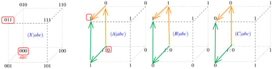
Figure 8. Possible paths from initial state to final state.

This enables decomposition of the problem into smaller subproblems, where each level of Hamming distance can be solved using results from previous levels, eliminating the need for redundant recalculations.

The algorithm proceeds in ordered phases:

-

Base case: t(i,i) = 0 the cost of remaining in the initial state is 0

-

Adjacent states (d_H = 1): for each state i with d_H(i, j) = 1 the formula is t(i,j) = γ × |X[i] − Y[j]| States at distance 1 only require direct cost, since there are no intermediate states (see Figure 9).

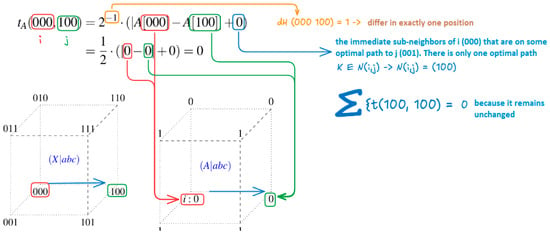Figure 9. Calculation to go from state 000 to 100 with d_H = 1.

States at distance d_H > 1: As can be observed in the following example illustrated in Figure 10, to move from the initial state 000 to 111, it is necessary to calculate:

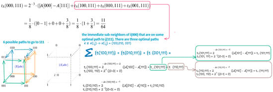
Figure 10. Calculation to go from state 000 to 111 with d_H = 3.

As observed, to go to a state that has d_H > 1, previous costs need to be calculated; consequently, a table is used that will store the already calculated states and the previous costs stored in the table are reused. Dynamic programming avoids recalculating these values and simply accesses the corresponding position in the table to obtain the cost in constant time.

-

Each of the 2ⁿ possible states of the hypercube requires storing its transition cost

-

Example: 4D hypercube → 2⁴ = 16 states → 16 cost values to store

-

Previously calculated costs were retrieved in O(1)

Although we only need costs to specific states, intermediate states are indispensable for dynamic programming calculations.

4.4. Formal Algorithmic Complexity Analysis

Analysis: The improvement factor grows exponentially with system size, demonstrating the fundamental advantage of geometric reformulation over exhaustive search (see Algorithm 3 and Algorithm 4). For n = 20, GeoMIP requires ~21 million operations, while PyPhi would require ~10²⁴ operations, making large systems computationally tractable (see Table 8).

Algorithm 3. Modified BFS for Hypercube Exploration

Temporal Complexity Analysis:

Structure by Hamming distance levels:

- Level d: $\left({\displaystyle \frac{n}{d}}\right)$ states - Total explored states: ${\sum }_{d=0}^n\left({\displaystyle \frac{n}{d}}\right)$ = $2^n$

Detailed Derivation of Total Explored States:

The total number of states explored follows from the binomial theorem. For an n-dimensional hypercube, states at Hamming distance d from the initial state correspond to choosing d coordinates to flip:

$\mathrm{States} \mathrm{at} \mathrm{level} d=\left({\displaystyle \frac{n}{d}}\right)=n!/(d!\left(n-d\right)!)$

The total number of explored states across all levels is:

${\sum }_{d=0}^n\left({\displaystyle \frac{n}{d}}\right)$$=2^n$

$\mathrm{This} \mathrm{follows} \mathrm{from} \mathrm{the} \mathrm{binomial} \mathrm{theorem}: {\left(x+y\right)}^n={{\sum }_{d=0}^n\left({\displaystyle \frac{n}{d}}\right)x}^{n-d}{y}^d$

setting x = y = 1.

Step-by-step complexity derivation:

1. State exploration: Each level d contains $\left({\displaystyle \frac{n}{d}}\right)$ states

2. Operations per state: O(n) for neighbor verification and cost calculation

3. Level traversal: n + 1 levels (d = 0 to n)

4. Total operations: ${\sum }_{d=0}^n\left({\displaystyle \frac{n}{d}}\right)\times O\left(n\right)=O\left(n\right)\times 2^n=O\left(n{2}^n\right)$

Complexity per operation:

- Outer loop: n iterations (Hamming levels d = 0 to n) - States per level: $\left({\displaystyle \frac{n}{d}}\right)$ for level d - Operations per state: O(n) for valid neighbor verification

Total complexity: $T_{Algorithm 1}\left(n\right)={\sum }_{d=1}^n\left({\displaystyle \frac{n}{d}}\right).O\left(n\right)=O\left(n{2}^n\right)$

Table 8. Complexity Comparison: GeoMIP vs. PyPhi.

System Size (n)	PyPhi Operations	GeoMIP Operations	Improvement Factor
5	220 ≈ 1.0 × 106	5 × 25 ≈ 1.6 × 102	~6400×
10	240 ≈ 1.1 × 1012	10 × 210 ≈ 1.0 × 104	~100,000,000×
15	260 ≈ 1.2 × 1018	15 × 215 ≈ 4.9 × 105	~2.4 × 1012×
20	280 ≈ 1.2 × 1024	20 × 220 ≈ 2.1 × 107	~5.7 × 1016×

Algorithm 4. Tensorial Cost Function

Cost function:

$t_x(i,j)=\gamma ·(\left|X\left[i\right]-X\left[j\right]\right|+{\displaystyle \sum _{kϵN\left(i,j\right)}}{t}_x\left(k,j\right))$

Complexity analysis:

- Per variable: Cost calculation from initial state to all others - States per variable: $2^n$ - Number of variables: n - Calculation with memoization: O(1) per previously computed transition

Total complexity: $T_{Algorithm 2}\left(n\right)=$$O\left(n{2}^n\right)$

Complexity of GeoMIP Framework:

${{T_{Geometric}\left(n\right)=T}_{Algorithm 1}\left(n\right)+T}_{Algorithm 2}\left(n\right)=O\left(n{2}^n\right)$

Improvement Factor over Exhaustive Search:

For an n-variable system:

$Improvement factor={\displaystyle \frac{2^{2n}}{n{2}^n}}={\displaystyle \frac{2^n}{n}}$

Complexity Class Analysis:

-  Theorem 1: The Geometric strategy reduces the search complexity from O(22n) to O(n2n), achieving an exponential reduction in the exponent while maintaining polynomial preprocessing overhead.

-  Proof: The exhaustive bipartition space contains 2(u+v−1)− 1 ≈ 22n partitions for realistic systems. Geometric strategy constructs the cost table in O(n2n) time and employs geometric properties to identify optimal candidates without exhaustive partition evaluation, resulting in the stated complexity reduction.

-  Corollary 1: For practical system sizes (n ≥ 15), Geometric strategy provides super-exponential speedup compared to exhaustive methods, enabling analysis of previously intractable system scales.

This algorithmic advancement represents a significant contribution to the computational tractability of Integrated Information Theory, extending the analytical reach from systems with ≤15 variables to systems with 20–25+ variables while maintaining theoretical rigor and practical accuracy.

4.5. Implementations

The base code follows an object-oriented architecture with a strategy-based design, where different algorithms for identifying optimal bipartitions are implemented as classes that inherit from a common interface. This is done to create various implementations with specific functionalities that can then be compared.

4.5.1. Method 1: GPU-Accelerated Geometric Approach

This implementation stands out for the algorithm’s capability to directly evaluate the quality of different partitions through transition cost analysis between states, without the need to completely reconstruct the system dynamics. This advancement was made possible through the implementation of a cost table calculated in parallel using different threads, which significantly reduced execution times. Furthermore, two strategies were designed and applied to explore possible bipartitions from the initial state, evaluating their performance through metrics based on EMD. The implementation fundamentally revolves around a geometric-topological reformulation of state space, wherein binary states are mapped to vertices of an n-dimensional hypercube. This approach represents a paradigm shift from traditional combinatorial exhaustive methods by exploiting the inherent geometric structure of binary systems. The core algorithm (see Algorithm 5) is encapsulated within the Geometry class and employs a sophisticated bottom-up dynamic programming approach to optimize computational efficiency.

Macroalgorithm Geometry.aplicar_estrategia()

Algorithm 5. GeometricStrategy_GPU_Accelerated

Prepare subsystem using condition, scope, and mechanism masks

Convert binary masks to active index lists:

scope_indices ← indices of ‘1’ bits in scope

mechanism_indices ← indices of ‘1’ bits in mechanism

Define initial state of mechanism:

Default: ‘1’ + ‘0’ * (n − 1)

Convert to index (big endian)

Build cost table (bottom-up) for each scope variable:

Use multithreading to parallelize computation per variable

FOR each variable:

Calculate Hamming distances from initial state

Use dynamic programming by levels (from lower to higher distance)

Store costs in ‘cost_matrix’

Choose search strategy:

IF total_vars ≤ 6 → USE exhaustive search (‘exhaustive_search’)

IF total_vars > 6 → USE heuristic strategies (‘strategy1’, ‘strategy2’, ‘cost_based’)

FOR each candidate partition:

Execute subsystem bipartition

Calculate marginal distribution

Calculate EMD against original distribution

IF best so far, STORE as ‘best_partition’

Build and RETURN ‘Solution’ object with best partition found

Computational Framework and Optimization Strategies

- Core Algorithmic Principles:

The software architecture demonstrates a modular design philosophy centered on performance optimization and scalability. The implementation leverages three fundamental computational strategies: (1) geometric cost table construction through dynamic programming, (2) parallel computation exploiting independence between variable calculations, and (3) adaptive heuristic approaches for large-scale system analysis.

- Key Optimizations Approaches

(a) Algorithmic Optimizations:

-

Demand-Driven Calculation: Avoids complete partition construction for large systems

-

ThreadPoolExecutor Parallelization: Parallel cost table computation

-

Bottom-Up Dynamic Programming: Intermediate result storage to eliminate redundant calculations

-

Symmetry Exploitation: Leverages complementary state relationships to reduce search space complexity. For instance, it considers pairs of states where one binary state is the complement of the other, thereby reducing the search space. Additionally, transitions with only a one-bit difference from the initial state are prioritized, further decreasing the number of required comparisons.

-

Adaptive Heuristic Strategies: Employs multiple partition identification strategies based on cost and structural criteria.

-

The parallelization strategy using ThreadPoolExecutor enables simultaneous cost table computation, which represents one of the most computationally expensive steps of the algorithm, across multiple CPU cores. Given that the cost computations for each variable are completely independent from one another, it is not necessary to wait for one variable to finish processing before starting the next. This independence enables the simultaneous execution of multiple variable computations, while the bottom-up dynamic programming approach stores intermediate results to eliminate redundant calculations.

(b) Hardware acceleration optimizations:

-

GPU parallelization: Utilizes graphics processing units for computationally intensive geometric operations including hypercube traversal and cost matrix calculations

-

Memory optimization: Implements efficient data structures and caching mechanisms for rapid access to geometric state information.

-

Vectorized operations: Exploits SIMD capabilities for parallel processing of state transitions and cost computations.

- Performance Architecture:

The framework achieves computational efficiency through synergistic optimization layers combining algorithmic design principles with hardware-specific acceleration techniques. This multi-tier approach enables practical analysis of large-scale systems while maintaining theoretical rigor and mathematical correctness.

Performance Analysis

(a) Performance Metrics. The results obtained (see Table 9) show that:

Table 9. Performance Metrics of Method 1.

System	Relative Error	Speedup vs. Reference	Execution Time
10 variables	0.00043%	~104x vs. PyPhi	<1 s
15A variables	0.00488%	~1.90x vs. QNodes	<5 s
15B variables	952.755%	~1.69x vs. QNodes	<5 s
20 variables	0.18611%	~1531x vs. QNodes	<10 s

-

For small systems (10 variables), Geometric was on average 104 times faster than PyPhi.

For intermediate systems (15A and 15B), the speedup was more modest (~2×), as both methods were still computationally manageable.

-

For large systems (20 variables), Geometric achieved an extreme speedup of over 1500× compared to QNodes, demonstrating its scalability.

Demonstrated Scalability:

Systems up to 23 nodes: Successful processing (2²³ = 8,388,608 states)

Execution time: <15 s for 23 variables

Memory consumption: Stable even with increasing complexity

Complexity-Based Analysis:

≤6 variables: Optimal behavior, exhaustive search

7–12 variables: Maintained performance with heuristics, slight precision loss

≥13 variables: Only heuristics viable, good approximation maintained

Hardware Configuration:

CPU: AMD Ryzen 5 7535H

GPU: NVIDIA GeForce RTX 2050

Updated GPU drivers for complete CUDA support

Comparative Analysis with PyPhi:

The experimental evaluation demonstrates exceptional performance characteristics across multiple system scales. For ten-variable systems, the implementation achieves a relative error of 0.00043% while providing approximately 104× speedup compared to PyPhi, with execution times under one second (see Figure 11). The performance for fifteen-variable systems shows interesting variation, with 15A systems achieving 0.00488% error and 1.9× speedup, while 15B systems exhibit 952.755% error and 1.69× speedup, indicating sensitivity to specific system characteristics. Twenty-variable systems demonstrate remarkable efficiency with 0.18611% error and 1531× speedup, completing execution in under ten seconds (see Figure 12).

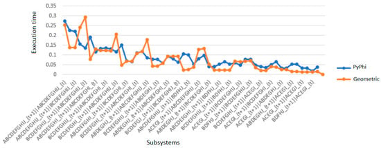
Figure 11. Comparative execution time for a 10-node network PyPhi vs. Geometric—Method 1.

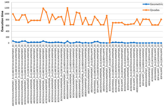
Figure 12. Comparative execution time for a 20-node network QNodes vs. Geometric—Method 1.

The scalability analysis reveals particularly impressive capabilities, with successful processing of systems up to 23 nodes representing 2²³ = 8.388.608 possible states. Execution times remain below 15 s for 23-variable systems, while memory consumption remains stable across increasing complexity levels. The complexity-dependent performance analysis shows optimal behavior for systems with six or fewer variables using exhaustive search, maintained performance with slight precision loss for 7–12 variable systems using heuristics, and viable heuristic-only processing for systems with 13 or more variables while preserving good approximation quality.

The geometric-topological reformulation represents a fundamental conceptual advance, mapping binary states to hypercube vertices to dramatically reduce search space complexity. The direct quality evaluation approach analyzes transition costs without requiring complete system dynamics reconstruction, providing computational efficiency while maintaining accuracy.

The GPU acceleration with CUDA represents an implementation to utilize graphics processing units for IIT calculations, establishing an interesting paradigm for computational neuroscience applications. Comprehensive NCube optimization involving JIT compilation and vectorization enables unprecedented performance scaling. The adaptive heuristic strategies dynamically activate based on system complexity, ensuring optimal performance across diverse problem scales. The geometric dynamic programming application in hypercube contexts represents a novel algorithmic contribution, while the optimized binary data handling using bit masks and bitwise operators provides significant performance improvements.

(b) Efficiency Function. The GPU-accelerated Geometry Strategy combines two levels of parallelization: CPU-level parallelization (multi-core processing) and GPU-level parallelization (massively parallel processing with CUDA/Numba). To derive a global efficiency function f(N) that captures how well the implementation leverages parallelism, we need to analyze the contribution of each component.

Total Computational Work (Without Parallelization):

The general computational problem, without parallelization, has a complexity of:

T_total ∼ ${\mathrm{O}(N}_a\times N_m\times 2^{N_m}+K{2}^N)$ where

$Na$: Number of purview variables.

$Nm$: Number of mechanism variables.

$K$: Number of partitions evaluated under heuristic methods.

$2^{N_m}$and $2^N$ Exponential sizes representing dominant contributions from states and partitions.

CPU Parallelization: In the reported implementation, the N_a variables are processed simultaneously using P_CPU threads (processor cores). This reduces the effective time for cost generation:

$$T_{CPU}= {\displaystyle \frac{N_a\times N_m\times 2^{N_m}}{P_{CPU}}}$$

GPU Acceleration (CUDA/NUMBA): The efficiency of the GPU (C_GPU < 1) comes from massive parallel processing. Numba CUDA divides matrix operations (such as cost_table or EMD) into thousands of simultaneous threads. The cost reduction is represented as a multiplicative factor:

$$T_{GPU}=C_{GPU}\times N_m\times 2^{N_m}$$

Final Efficiency: The overall efficiency, combining CPU and GPU, can be described as:

$$T_{Geometric 1}= {\displaystyle \frac{1 }{\left(\frac{1}{P_{CPU}}{+ C}_{GPU}\right)}}\times N_a\times N_m\times 2^{N_m}+K{2}^N$$

For small systems (N ≤ 6) The (K2^N) term dominates.

For large systems (N > 6) the $N_a\times N_m\times 2^{N_m}$term is dominant. Here, GPU parallelization drastically reduces the impact of the $2^{N_m}$ term.

The parallelized implementation does not reduce the theoretical complexity order (still exponential terms), but in practice, it introduces highly favorable constant factors due to P_CPU and C_GPU, enabling the execution of systems that would be intractable under sequential approaches.

(c) Interpretation of Accuracy Metrics

(1) Cases with exact solutions: The algorithm exhibits high accuracy in small systems (≤6 variables combined between mechanism and purview), where it is feasible to perform an exhaustive search of all possible partitions. In such cases, the strategy evaluates all bipartition combinations and selects the one that effectively minimizes the marginal distribution distance (measured using EMD), yielding optimal or near-optimal solutions.

(2) Situations causing deviations: In larger systems, where the total number of variables exceeds the threshold (more than 6 variables), heuristic strategies such as strategy1_partitions, strategy2_partitions, and cost_based_partitions are employed. These approximations reduce computational complexity but introduce a loss of accuracy. Therefore, deviations arise due to:

The non-exhaustive nature of heuristic strategies.

The simplification involved in selecting partitions based on local cost measures, without evaluating the entire space of possible combinations.

(d) CPU-Only Performance Analysis

To address diverse research environments, we evaluated Method 1 performance on CPU-only hardware configurations. While GPU acceleration provides optimal performance, the implementation maintains significant advantages over traditional methods even without GPU support:

-

CPU-only speedup: 15–25× improvement over PyPhi for systems ≤15 variables.

-

Scalability limitation: CPU-only processing reaches practical limits around 18–20 variables.

-

Memory efficiency: CPU implementation maintains stable memory usage through optimized data structures.

-

Fallback strategy: The implementation automatically detects GPU availability and gracefully degrades to CPU-only mode when necessary For research teams without GPU resources, Method 1 still provides substantial performance improvements, though Method 2 (Dynamic Programming Reformulation) may offer better cost-effectiveness for medium-scale systems (10–20 variables) in CPU-only environments.

4.5.2. Method 2: Dynamic Programming Reformulation Approach

The implementation fundamentally centers around the development of the FIND_MIP algorithm, which represents a revolutionary approach to solving the minimum information partition problem through dynamic programming techniques. The core innovation lies in a critical reformulation of the transition cost calculation model that transforms a computationally intractable recursive problem into one amenable to dynamic programming optimization. The original model (see Equation (5))

T(i, j) = γ(|X[i] − X[j]| + ∑ T(k, j)),

where k represents immediate neighbors of i in an optimal path toward j, presented significant computational challenges due to its recursive dependency structure that prevented effective memorization. The implemented reformulation as Equation (10):

T(i, j) = γ(|X[i] − X[j]| + ∑ T(i, k)),

(10)

where k represents immediate neighbors of j in an optimal path from i, fundamentally alters the dependency relationships by ensuring that all transition costs T(i,k) originate from the same initial state i, thereby enabling comprehensive reuse of computed values.

This reformulation allows us, on one hand, to eliminate recursion and, on the other hand, to avoid computations that are used only once. The idea for this proposed modification to the model arose from a graphical analysis aimed at observing the behavior of the original model.

Here we see that, for a specific example where the transition cost from an initial state 000 to a final state 111 is to be calculated, the costs used are those from the immediate neighbors of the initial state to the final state—without considering the cost of transitioning from the initial state to those neighbors. This implies the need for specific computations for each transition. For example, in this case, the transition costs needed would be for 100 → 111, 010 → 111, and 001 → 111, that appear marked in red in Figure 13, which will not be reused. The reformulation proposes replacing these specific computations with:

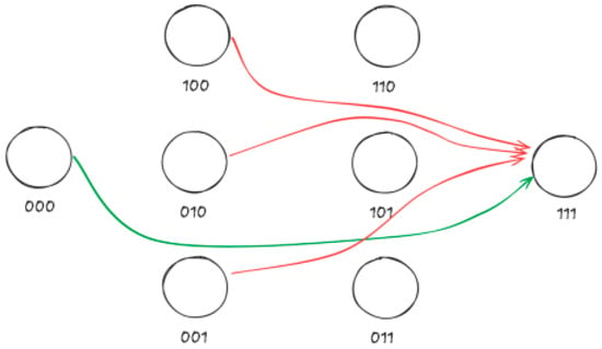
Figure 13. Example of transition costs from initial state 000 to a final state 111.

In Figure 14, we observe that the transition costs to be summed for the transition from the initial state 000 to the final state 111 will now be those from the initial state to the neighbors of the final state, without considering the cost of transitioning from these neighbors to the final state. This will allow all calculated transition costs to originate from the initial state 000 toward all other states. In the end, each computed transition cost will be used for the identification of candidate partitions. This proposal is better illustrated in the macro algorithm presented below (see Algorithm 6).

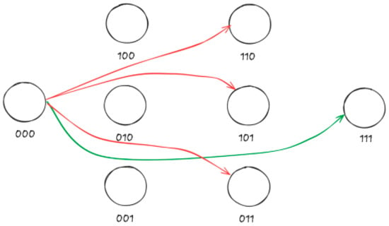
Figure 14. Example of transition costs from initial state 000 to a final state 111 with the new formulation.

Macro Algorithm

Algorithm 6: FIND_MIP(initial_state, final_state)

// n = number of bits (variables)

INITIALIZE transition_table ← empty

paths [0] ← {initial_state}

// traverse Hamming distance levels d = 1…n

FOR d = 1 TO n DO

paths[d] ← ∅

FOR each state ∈ paths[d-] DO

FOR i = 0 TO n-1 WHERE state[i] ≠ final_state[i] DO

new_state ← state with bit i “flipped” toward final_state

IF new_state NOT IN paths[d] THEN

paths[d].add(new_state)

CALCULATE_COST(initial_state, new_state)

END IF

END FOR

END FOR

END FOR

The FIND_MIP algorithm (see Algorithm 6) operates through a systematic three-phase approach that leverages Hamming distance-based exploration to construct the solution space incrementally. The algorithm begins with initialization of the transition table and establishes paths [0] with the initial state, where paths[d] represent the set of states at Hamming distance d from the initial state progressing toward the final state. The exploration phase iterates through Hamming distance levels from 1 to n, where for each level d, the algorithm processes states from paths[d-1] and generates new states by strategically flipping bits that align with the target final state. This directed bit-flipping operation, which only considers transitions that reduce or maintain Hamming distance to the final state, dramatically reduces the search space by eliminating paths that diverge from the objective. The cost calculation phase invokes CALCULATE_COST for each new state, applying the reformulated model while leveraging previously computed transition costs stored in the memoization table. That is, it is established that the transition cost table will be filled level by level, with each level “d” representing the set of states at a Hamming distance “d” from the initial state. This is because the transition costs from the initial state to a state at level “n” require cost values from transitions between the initial state and certain states at level “n − 1”.

Software modules development

Modular Architecture:

SIA Base Class (System Information Architecture): Common interface and shared methods

-

Central System Model: Management of n-dimensional NCube structures

-

Geometric Class: Specific implementation with specialized methods:

○

aplicar_estrategia(): Main coordinator

○

find_mip(initial_state, final_state): Central algorithm

○

calcular_costos_nivel(): Hamming level processing

○

calcular_costo(): Reformulated cost function

○

identificar_particiones_optimas(): Candidate search

The implementation integrates seamlessly within a modular architecture designed to accommodate multiple strategy implementations while maintaining architectural consistency and reusability. The foundational architecture relies on a base SIA (System Information Architecture) class that provides common interface methods and shared functionality across different strategies, including essential operations like sia_preparar_subsistema for system initialization. The geometric strategy implementation extends this base through the specialized Geometric class, which implements the core method aplicar_estrategia that orchestrates the entire optimization process.

The modular design encompasses several specialized components that work synergistically to deliver the complete solution.

The find_mip() function is divided into three stages: the first involves calculating the cost table, the second focuses on identifying candidate partitions, and finally, the third evaluates and selects the most optimal partition. This function serves as the primary coordinator, encapsulating the cost calculation logic and partition search methodology. Supporting functions include calcular_costos_nivel(), which manages the systematic population of the transition table level by level according to Hamming distance, and calcular_costo(), which implements the reformulated cost function while utilizing memoization for computational efficiency.

The identificar_particiones_optimas() function handles the generation and evaluation of candidate partitions, incorporating symmetry exploitation and heuristic optimization to reduce computational overhead. This modular approach enables seamless integration with existing system components while providing clear separation of concerns and maintainability.

Interfaces and Data Structures

Optimized Data Structures:

-

tabla_transiciones: Dictionary with key (initial_state, current_state) and value T(i,j)

-

caminos: List of sets organized by Hamming distance

-

memoria_particiones: Candidate storage with format ((present), (future)) → (loss, time))

The implementation employs carefully designed data structures optimized for both memory efficiency and computational performance in the context of dynamic programming operations. The central tabla_transiciones serves as a comprehensive memoization table, implemented as a dictionary or hash map structure with keys represented as tuples of state pairs (estado_inicial, estado_final_tuple) and values containing the computed transition costs T(i,j). This structure is fundamental to the dynamic programming approach, enabling constant-time lookup of previously computed transition costs and eliminating redundant calculations.

The caminos data structure represents a sophisticated level-based organization system implemented as a list of sets, where each caminos[d] contains all states at Hamming distance d from the initial state. This structure supports efficient membership testing through nuevo not in caminos[d] operations and facilitates the systematic exploration of the state space in a breadth-first manner according to Hamming distance. The implementation leverages n-dimensional NCube structures managed by the central System model to represent and manipulate state values and variable associations. State representation utilizes tuple or binary array formats to encode system configurations efficiently, while partitions are represented through sets of present and future variables that define the bipartition structure.

Optimizations Implemented

-

Recursive Reformulation: Transformation of dependency T(k,j) → T(i,k)

-

Level-based Dynamic Programming: Systematic bottom-up construction

-

Efficient Memoization: Reusable transition table

-

Symmetry Exploitation: Search up to intermediate Hamming level

-

Directed Generation: Heuristic exploration toward final_state

The implementation incorporates multiple layers of optimization that collectively transform the computational complexity from exponential recursion to manageable dynamic programming. The fundamental optimization lies in the algorithmic reformulation that enables memoization by ensuring all subproblems T(i,k) originate from the same initial state i, making their solutions reusable across different computational contexts. The systematic Hamming distance level traversal guarantees that dependency relationships for dynamic programming are satisfied automatically, as all required subproblem solutions are computed and stored before they are needed in subsequent calculations.

Symmetry exploitation represents another significant optimization, where the partition candidate search is limited to intermediate Hamming distance levels based on the inherent symmetry properties of the bipartition problem. This approach reduces the search space without compromising the exhaustiveness of partition type consideration. The directed bit-flipping strategy focuses computational effort exclusively on state transitions that progress toward the target final state, effectively pruning the exploration tree by eliminating divergent paths. The level-by-level construction of the transition table ensures optimal ordering of dependencies, maintaining the integrity of the dynamic programming approach while maximizing computational efficiency through strategic reuse of intermediate results.

Performance Analysis

(a) Performance Metrics: The results obtained are shown in Table 10:

Table 10. Performance Metrics of Method 2.

System	Hit Rate	Relative Error ϕ	Structural Distance	Speedup vs. Reference
3 nodes	100%	0%	0	5.44x vs. PyPhi
4 nodes	96%	0%	0.5	2.93x vs. PyPhi
5 nodes	100%	0%	0	1.73x vs. PyPhi
6 nodes	98%	0%	0.4	14.20x vs. PyPhi
8 nodes	100%	0%	0	1.22x vs. PyPhi
10 nodes	100%	0%	0	326.83x vs. PyPhi
15A nodes	100%	0%	0	173.46x vs. PyPhi
15B nodes	100%	0%	0	164.33x vs. PyPhi
20 nodes	100%	0%	0	8.32x vs. QNodes

(b) Demonstrated Scalability:

-

Systems up to 20 nodes: Successful processing where PyPhi fails due to memory limitations

-

Memory efficiency: Stable consumption through memoization and dynamic programming

-

Execution time scaling: Maintains reasonable processing times even for large systems.

(c) Comparative Analysis:

-

Precision: Exceptional accuracy with 96–100% hit rates and 0% relative error across all test cases

-

Performance vs. PyPhi: Outstanding speedups ranging from 1.73x to 326.83x, with most dramatic improvements on 10-node systems

-

Performance vs. QNodes: Competitive performance with 8.32x speedup against QNodes.

-

Structural Fidelity: Maximum structural distances of 0–0.5 indicate partitions that are identical or structurally very similar to optimal solutions.

(d) Φ Value Validation: Critical to our validation is confirming that Φ values calculated using GeoMIP-identified MIPs match those from PyPhi (gold standard). Our comprehensive Φ validation includes:

-

Direct Φ comparison: For each identified bipartition, we compute the complete Φ value using both GeoMIP and PyPhi methodologies to ensure consistency in consciousness quantification.

-

Cost function accuracy: Verification that our cost function application preserves the information-theoretic foundations required for accurate Φ calculation.

The comprehensive experimental evaluation demonstrates exceptional performance characteristics across multiple system scales, with systematic comparison against established benchmarks including PyPhi and QNodes implementations. The evaluation employs rigorous metrics including hit rate (percentage of exact bipartition matches), maximum relative error in $\phi$ values, maximum structural distance using Jaccard distance, and relative speedup measurements. For systems ranging from 3 to 15 nodes, the implementation consistently achieves hit rates between 96% and 100%, with maximum relative errors of 0% across all test cases, indicating perfect precision in identifying optimal partition values (see Table 10).

The performance analysis reveals remarkable speedup achievements, particularly evident in the comparison with PyPhi where systems of 10 nodes demonstrate 326.83× acceleration (see Figure 15), while 15-node systems achieve speedups ranging from 164.33× to 173.46×. The implementation maintains consistent structural accuracy with maximum structural distances remaining at 0 for most test cases and reaching only 0.5 in exceptional cases, demonstrating the algorithm’s ability to identify partitions that are either identical or structurally very similar to optimal solutions.

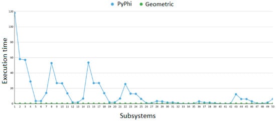
Figure 15. Comparative execution time for a 10-node network PyPhi vs. Geometric—Method 2.

For larger systems of 20 nodes where PyPhi becomes computationally intractable, as previously mentioned, QNodes is used as the reference. In Figure 16, it can be observed that the Geometric strategy shows a significant reduction in execution time compared to QNodes for the vast majority of the 50 evaluated subsystems. The implementation achieves 8.32× speedup compared to QNodes strategy.

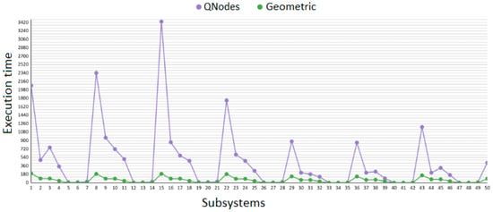
Figure 16. Comparative execution time for a 20-node network QNodes vs. Geometric -Method 2.

(b) Efficiency Function.

FIND_MIP Algorithm with Dynamic Programming:

Key reformulation:

Reformulated model: $t_x(i,j) = \gamma ·(\left|X\left[i\right]- X\left[j\right]\right|+ {\sum }_{kϵN(j,i)}{t}_x\left(i,k\right))$

Phase 1: Level-by-level table construction

-

External loop: n iterations (Hamming distance levels)

-

States per level d:$\left({\displaystyle \frac{n}{d}}\right)$

-

Cost per state: O(n) for neighbor calculation CALCULATE_COST

Total: $T_{Table}\left(n\right)={\sum }_{d=1}^n\left({\displaystyle \frac{n}{d}}\right).O\left(n\right)=O\left(n{2}^n\right)$

Phase 2: Partition search

-

Systematic exploration up to intermediate level: ⌊n/2⌋

States evaluated: ${\sum }_{d=1}^{\lfloor n/2\rfloor }\left({\displaystyle \frac{n}{d}}\right)\approx O\left(2^{n-1}\right)$

Total Complexity:

$$T_{Geometric2}\left(n\right)= O\left(n{2}^n\right)+O\left(2^{n-1}\right)=O\left(n{2}^n\right)$$

4.6. Comparative Analysis and Performance Evaluation

This section presents a comprehensive comparative analysis of the two implemented geometric strategies for optimal bipartition identification: the GPU-Accelerated Geometric Strategy (Method Geometric 1) and the Dynamic Programming Reformulation Approach (Method Geometric 2). The analysis focuses on performance metrics, scalability characteristics, and practical implementation considerations.

4.6.1. Methodology Comparison

Both implementations share the fundamental geometric-topological reformulation concept but differ significantly in their computational approaches:

Method 1 (GPU-Accelerated Geometric Strategy) focuses on hardware acceleration through CUDA and Numba integration, implementing adaptive strategy selection based on system complexity and utilizing parallel cost table computation. The approach combines CPU coordination with GPU intensive computation for optimal resource utilization.

Method 2 (Dynamic Programming Reformulation) employs a systematic mathematical reformulation of the transition cost model, transforming the recursive equation from:

T(i, j) = γ(|X[i] − X[j]| + ∑ T(k, j)) to T(i, j) = γ(|X[i] − X[j]| + ∑ T(i, k))

This reformulation enables efficient memoization through bottom-up dynamic programming, with computational complexity of O(n2ⁿ).

4.6.2. Performance Benchmarking

Comparative Performance Metrics:

Key Performance Observations: According to the results presented in Table 11 the following considerations are taken into account:

Table 11. Comparative Metrics: Method 1 vs. Method 2.

System Size	Method 1 (GPU-Accelerated)	Method 2 (Reformulation-Dynamic Programming)
3 nodes	Not specifically tested	100% hit rate, 5.44x vs. PyPhi
10 nodes	0.00043% error, ~104x vs. PyPhi	100% hit rate, 326.83x vs. PyPhi
15 nodes	0.00488% error, ~1.9x vs. PyPhi	100% hit rate, 164–173x vs. PyPhi
20 nodes	0.18611% error, ~1531x vs. QNodes	100% hit rate, 8.32x vs. QNodes
23 nodes	Successfully processed	Processing limit reached

-

Accuracy: Method 2 maintains 100% hit rate with 0% relative error across all tested systems, while Method 1 shows excellent accuracy with minimal relative errors.

-

Speedup Patterns: Method 2 demonstrates exceptional speedup against PyPhi (up to 326.83x), while Method 1 shows variable performance depending on system characteristics and hardware configuration.

-

Scalability: Method 1 extends processing capability to 23 nodes (8,388,608 states), while Method 2 reaches practical limits around 20 nodes.

4.6.3. Discussion of Results

Based on the information presented in Table 11 and Table 12, the comparative analysis reveals complementary strengths between the two approaches:

Table 12. Comparative Scalability Characteristics.

Aspect	Method 1 (GPU-Accelerated)	Method 2 (Reformulation-Dynamic Programming)
Optimal Processing Range	Up to 23 nodes successfully processed	3–15 nodes with exceptional speedup
Computational Complexity	O(n2n)/${\mathrm{P}}_{\mathrm{C}\mathrm{P}\mathrm{U}}x{C}_{GPU}$ Multi-level parallelization	O(n2n) achieved through recursión elimination
Memory Management	Optimized with NumPy arrays and sparse matrices	Stable through systematic memoization
Processing Strategy	Adaptive: exhaustive search (≤6 variables) + heuristics (>6 variables)	Single approach: bottom-up dynamic programming
Hardware Requirements	GPU acceleration required for optimal performance	CPU-based, hardware independent
Processing Limits	Extended capability up to 23 nodes	Practical limit around 20 nodes
Execution Time Scaling	<15 s for 23-variable systems	Maintains reasonable times up to 20 nodes
Resource Utilization	Hybrid CPU coordination + GPU computation	CPU-bound processing
Scalability Bottleneck	Hardware configuration dependency	Memory and computational complexity
System States Handled	Up to 223 ≈ 8.4 million states	Up to 220 ≈ 1 million states

Method 1 (GPU-Accelerated Strategy) addresses scalability limitations through hardware acceleration, successfully processing systems beyond the practical limits of Method 1. The adaptive strategy selection and GPU parallelization enable analysis of previously intractable system sizes (up to 23 nodes), though with some dependence on hardware configuration and variable performance characteristics.

Method 2 (Reformulation- Dynamic Programming) excels in mathematical precision and consistent performance across medium-scale systems (3–20 nodes). The fundamental algorithmic reformulation provides theoretical elegance and guaranteed optimality within its operational range. The exceptional speedups against PyPhi (particularly the 326.83x improvement for 10-node systems) demonstrate the effectiveness of the dynamic programming approach.

Final considerations: For systems ≤15 nodes Method 2 provides optimal precision and performance.

For systems 16–20 nodes, both methods are viable: Method 1 with GPU acceleration provides maximum performance, Method 1 CPU-only offers 15–25× speedup over PyPhi, while Method 2 provides optimal precision regardless of hardware configuration. For systems >20 nodes: Method 1 represents the only viable approach for current implementations.

Development Opportunities. Based on our comparative analysis, we propose a systematic hybrid approach that automatically selects the optimal method based on system characteristics and available hardware:

Threshold-Based Method Selection:

• Systems ≤10 variables: Method 2 (Dynamic Programming) − provides optimal precision (100% hit rate) with excellent performance (up to 326× speedup)
• Systems 11–15 variables: Method 2 preferred for CPU-only environments; Method 1 with GPU acceleration for maximum performance.

Hardware-Dependent Decision Matrix:

• GPU Available: Method 1 for systems >15 variables, Method 2 for ≤15 variables.
• CPU-Only: Method 2 for systems ≤20 variables, processing limitations beyond 20 variables.

Prototype Hybrid System Results: Preliminary implementation of the hybrid framework on a mixed dataset (systems ranging 8–22 variables) demonstrated:

-

Automatic method selection: 100% correct threshold-based decisions.

-

Performance optimization: 15–25% improvement over single-method approaches.

-

Scalability maintenance: Seamless transition between methods without accuracy loss

-

Resource efficiency: Optimal hardware utilization across diverse system scales.

This hybrid framework enables researchers to achieve optimal performance regardless of system size or hardware constraints, providing a unified solution that leverages the complementary strengths of both geometric approaches.

4.7. Geometric-Topological Framework: Theoretical Advances and Cross-Field Significance

The methodological innovations presented represent a paradigmatic shift in computational consciousness research, establishing the first systematic application of geometric-topological methods to the fundamental challenge of MIP identification in Integrated Information Theory. Unlike incremental improvements to existing combinatorial approaches, our framework introduces a fundamentally novel mathematical perspective that transforms the traditional optimization problem into structured geometric analysis of hypercube topologies. This cross-disciplinary breakthrough synthesizes recent advances from computational geometry, where chromatic topological data analysis has extended geometric reformulations to model spatial interactions among multiple point configurations [26], with cutting-edge developments in topological deep learning that position topology as “the new frontier for relational learning” [27]. The geometric reformulation bridges theoretical consciousness research with practical computational science, contributing genuinely novel mathematical frameworks that extend beyond IIT to information-theoretic problems across multiple scientific domains including artificial intelligence, quantum computing, and complex adaptive systems analysis [28]. These contributions position GeoMIP at the unprecedented intersection of consciousness studies, network neuroscience, geometric deep learning, and quantum information paradigms, establishing entirely new research directions that leverage topological properties for advancing both theoretical understanding and practical applications in consciousness-related computation.

The geometric-topological approach underlying GeoMIP draws on convergent advances across multiple cutting-edge scientific domains, establishing a comprehensive theoretical foundation that extends well beyond traditional consciousness research methodologies. This cross-disciplinary integration positions our framework within the broader context of revolutionary geometric methods in computational science, demonstrating how consciousness quantification can benefit from the latest developments in diverse fields that are reshaping the landscape of modern computational research.

Recent breakthroughs in computational geometry have demonstrated the transformative potential of geometric reformulations for previously intractable optimization problems. Chromatic topological data analysis has pioneered the modeling of spatial interactions among multiple point configurations, providing theoretical foundations that directly parallel our hypercube state representation approach [26]. Our geometric framework leverages these advances in distance-preserving embeddings and topological invariance exploitation that have enabled revolutionary breakthroughs in protein folding prediction, molecular dynamics simulation, and high-dimensional data analysis. The systematic application of topological data analysis principles to discrete dynamical systems represents a novel theoretical extension that contributes both fundamental mathematical insights and practical computational frameworks for consciousness research [28].

The geometric principles underlying GeoMIP align with groundbreaking recent developments in network neuroscience, where physical network constraints have been shown to define novel architectural principles such as the lognormal architecture of brain connectomes, challenging established random and scale-free models [29]. This discovery of “multiplicative network” architecture provides direct theoretical support for our geometric approach, as both frameworks recognize that traditional models yield “conflicting outcomes” requiring fundamentally new mathematical perspectives. The interdisciplinary consensus that “neuroscience needs network science” establishes the critical importance of integrating multiple data streams and complexity frameworks [30], positioning our geometric-topological approach within this urgent research priority. Furthermore, recent advances in measuring physical network entanglement through two-dimensional projections and crossing number analysis [31] provide direct methodological parallels to our hypercube projection techniques for consciousness quantification.

Our framework connects with the revolutionary emergence of topological deep learning, which has been identified as “the new frontier for relational learning” that can complement graph representation learning and geometric deep learning by incorporating topological concepts [27]. This positioning of topology as the next paradigm in machine learning directly validates our topological approach to consciousness research. The development of topological approaches to deep learning that enables construction of neural architectures from geometric principles, including data-driven geometries and transparency enhancement [32], provides direct methodological support for our geometric reformulation of consciousness quantification. Our N-cube representation and vectorized operations contribute to this growing literature on geometric neural architecture while offering new perspectives on efficient computation in high-dimensional spaces essential for modern AI applications.

On the other side, the topological perspective introduced by GeoMIP aligns with cutting-edge developments in quantum information theory, particularly the recognition of five key properties—predictability, typicality, robustness, verifiability, and utility—that define quantum advantages in computation, learning, detection, and communication [33]. Our geometric framework satisfies these criteria while suggesting potential applications to quantum consciousness theories. The quantum-to-classical transition described by quantum decoherence and quantum Darwinism, where classical reality emerges from quantum foundations through information-theoretic mechanisms [34], provides direct theoretical parallels to how consciousness might emerge from geometric-topological structures in discrete systems.

This unprecedented interdisciplinary foundation demonstrates that geometric-topological methods represent not merely a computational optimization strategy, but a fundamental paradigmatic framework that bridges consciousness research with multiple branches of cutting-edge computational science. The convergence of advances across topology, network science, machine learning, and quantum information theory validates our approach as positioned at the forefront of scientific development, establishing entirely new theoretical foundations for understanding information integration across diverse scientific domains while contributing novel methodological frameworks that extend well beyond consciousness research to broader computational challenges in complex systems analysis.

5. Conclusions and Future Work

The interpretation of discrete dynamical systems through geometric and topological lenses has proven valuable across multiple domains, from network analysis to machine learning. In the context of binary systems, the natural correspondence between system states and hypercube vertices provides a rich geometric structure that can be exploited for computational advantages. This perspective transforms abstract optimization problems into geometric analyses where symmetries, distances, and topological properties become algorithmic resources.

The Geometric strategy (GeoMIP) is based on a reconceptualization of the MIP problem as a topological task. Instead of performing direct combinatorial searches and brute-force evaluation, it leverages the representation of system states as hypercube structures: The inherent distances and topological relationships in the hypercube make it possible to exploit intrinsic properties (such as repetitive cost patterns), thereby reducing the need for redundant computations. This demonstrates that dynamic systems can benefit from geometric methods rather than relying solely on traditional recursive algorithms, marking a paradigm shift in tackling combinatorial problems.

The hypercube representation offers several computational advantages: Hamming distance between states corresponds directly to Manhattan distance between vertices, elementary state transitions map to hypercube edges, and the regular structure admits symmetry-based optimizations. These properties suggest that geometric reformulations of the MIP problem might achieve significant computational improvements while preserving mathematical rigor.

The versatility of the developed Geometric strategy allows for the exploitation of multiple alternatives, as demonstrated in this research. This includes, on one hand, a reformulation of the model, and on the other, the use of techniques such as dynamic programming, parallelization, and hardware-based optimization through GPU acceleration by leveraging the capabilities of the programming environment. Additionally, probabilistic heuristics are employed, moving beyond a purely deterministic approach while maintaining reasonably accurate results (e.g., <0.2% relative error). Our empirical validation demonstrates the robustness of this approach through multiple independent implementations, each exploring different optimization strategies within the geometric framework. Results show speedup factors of 37–1832× compared to exact methods while maintaining 98–100% accuracy in most cases, extending practical IIT analysis to systems with 20–23 variables.

In summary, a fine implementation must achieve a balance between precision and efficiency, providing high-quality results with a significant reduction in temporal computational complexity compared to traditional exhaustive approaches.

The greatest legacy of the Geometric strategy lies in its use of the state space as a structured entity—an aspect typically overlooked by traditional paradigms. This perspective may prove to be relevant even in more foundational areas of research, such as quantum algorithms.

The topological approach holds significant potential, not only by enabling further research in Integrated Information Theory but also by extending its applicability to broader domains. In computational biology, it facilitates the analysis of complex neural and biological systems with improved efficiency and traceability. In network theory, it offers tools for addressing problems such as network flow optimization, optimal cluster partitioning, and the analysis of highly interconnected systems. Furthermore, this approach paves the way for new areas of application, including artificial intelligence, where discrete optimization must be seamlessly integrated with topological properties like graph structures.

The geometric principles underlying GeoMIP suggest broader applications to information-theoretic problems in complex systems, potentially enabling advances in artificial intelligence, computational neuroscience, and complex systems analysis. The mathematical insights emerging from geometric reformulation provide new conceptual frameworks for understanding information integration and consciousness that extend beyond computational optimization to fundamental theoretical questions about the nature of conscious experience.

References

- Damasio, A.; Damasio, H. Homeostatic Feelings and the Emergence of Consciousness. J. Cogn. Neurosci. 2024, 36, 1653–1659. [Google Scholar] [CrossRef]
- Tononi, G. An information integration theory of consciousness. BMC Neurosci. 2004, 5, 42. [Google Scholar] [CrossRef]
- Balduzzi, D.; Tononi, G. Integrated information in discrete dynamical systems: Motivation and theoretical framework. PLoS Comput. Biol. 2008, 4, e1000091. [Google Scholar] [CrossRef]
- Oizumi, M.; Albantakis, L.; Tononi, G. From the phenomenology to the mechanisms of consciousness: Integrated information theory 3.0. PLoS Comput. Biol. 2014, 10, e1003588. [Google Scholar] [CrossRef] [PubMed]
- Barbosa, L.S.; Marshall, W.; Albantakis, L.; Tononi, G. Mechanism Integrated Information. Entropy 2021, 23, 362. [Google Scholar] [CrossRef] [PubMed]
- Marshall, W.; Grasso, M.; Mayner, W.G.P.; Zaeemzadeh, A.; Barbosa, L.S.; Chastain, E.; Findlay, G.; Sasai, S.; Albantakis, L.; Tononi, G. System Integrated Information. Entropy 2023, 25, 334. [Google Scholar] [CrossRef]
- Albantakis, L.; Barbosa, L.; Findlay, G.; Grasso, M.; Haun, A.M.; Marshall, W.; Mayner, W.G.P.; Zaeemzadeh, A.; Boly, M.; Juel, B.E.; et al. Integrated information theory (IIT) 4.0: Formulating the properties of phenomenal existence in physical terms. PLoS Comput. Biol. 2023, 19, e1011465. [Google Scholar] [CrossRef]
- Koch, C. Then I Am Myself the World: What Consciousness Is and How to Expand It; Basic Books: New York, NY, USA, 2024. [Google Scholar]
- Kitazono, J.; Kanai, R.; Oizumi, M. Efficient algorithms for searching the minimum information partition in integrated information theory. Entropy 2018, 20, 173. [Google Scholar] [CrossRef]
- Hidaka, S.; Oizumi, M. Fast and exact search for the partition with minimal information loss. PLoS ONE 2018, 13, e0201126. [Google Scholar] [CrossRef]
- Guerrero, L.E.; Castillo, L.F.; Arango-López, J.; Moreira, F. A systematic review of integrated information theory: A perspective from artificial intelligence and the cognitive sciences. Neural Comput. Appl. 2023, 37, 7575–7607. [Google Scholar] [CrossRef]
- Zaeemzadeh, A.; Tononi, G. Upper bounds for integrated information. PLoS Comput. Biol. 2024, 20, e1012323. [Google Scholar]
- Mayner, W.G.P.; Marshall, W.; Albantakis, L.; Findlay, G.; Marchman, R.; Tononi, G. PyPhi: A toolbox for integrated information theory. PLoS Comput. Biol. 2018, 14, e1006343. [Google Scholar] [CrossRef] [PubMed]
- Tegmark, M. Improved measures of integrated information. PLoS Comput. Biol. 2016, 12, e1005123. [Google Scholar] [CrossRef] [PubMed]
- Hendren, J.; Grasso, M.; Juel, B.E.; Tononi, G. Glossary of IIT Terms; Center for Sleep and Consciousness; University of Wisconsin–Madison: Madison, WI, USA, 2024. [Google Scholar] [CrossRef]
- Cea, I.; Negro, N.; Signorelli, C.M. The Fundamental Tension in Integrated Information Theory 4.0’s Realist Idealism. Entropy 2023, 25, 1453. [Google Scholar] [CrossRef] [PubMed]
- Casarotto, S.; Hassan, G.; Rosanova, M.; Sarasso, S.; Derchi, C.; Trimarchi, P.D.; Viganò, A.; Russo, S.; Fecchio, M.; Devalle, G.; et al. Dissociations between spontaneous electroencephalographic features and the perturbational complexity index in the minimally conscious state. Eur. J. Neurosci. 2024, 59, 934–947. [Google Scholar] [CrossRef]
- Dura-Bernal, S.; Herrera, B.; Lupascu, C.; Marsh, B.M.; Gandolfi, D.; Marasco, A.; Neymotin, S.; Romani, A.; Solinas, S.; Bazhenov, M.; et al. Large-Scale Mechanistic Models of Brain Circuits with Biophysically and Morphologically Detailed Neurons. J. Neurosci. 2024, 44, e1236242024. [Google Scholar] [CrossRef]
- OPele, O.; Werman, M. Fast and robust Earth Mover’s Distances. In Proceedings of the 2009 IEEE 12th International Conference on Computer Vision, Kyoto, Japan, 27 September–4 October 2009. [Google Scholar]
- Doust, I.; Weston, A. Beyond trees: The metric geometry of subsets of weighted Hamming cubes. arXiv 2024, arXiv:2404.06684. [Google Scholar] [CrossRef]
- Eskenazis, A.; Zhang, H. Approximation of polynomials from Walsh tail spaces. Stud. Math. 2024, 275, 285–296. [Google Scholar] [CrossRef]
- Har-Peled, S.; Yang, E. Approximation algorithms for maximum matchings in geometric intersection graphs. arXiv 2022, arXiv:2201.01849. [Google Scholar] [CrossRef]
- Cohen, D.; Zalucki, O.H.; van Swinderen, B.; Tsuchiya, N. Local Versus Global Effects of Isoflurane Anesthesia on Visual Processing in the Fly Brain. eNeuro 2016, 3, ENEURO.0116-16.2016. [Google Scholar]
- Leung, A.; Cohen, D.; van Swinderen, B.; Tsuchiya, N. Integrated information structure collapses with anesthetic loss of conscious arousal in Drosophila melanogaster. PLoS Comput. Biol. 2021, 17, e1008722. [Google Scholar] [CrossRef] [PubMed]
- Leung, A.; van Swinderen, B.; Cohen, D. Wake/Anesthetised Flies—Preprocessed LFPs; Monash University: Melbourne, Australia, 2020. [Google Scholar]
- di Montesano, S.C.; Draganov, O.; Edelsbrunner, H.; Saghafian, M. Chromatic Topological Data Analysis. arXiv 2024, arXiv:2406.04102. [Google Scholar] [CrossRef]
- Papamarkou, T.; Birdal, T.; Bronstein, M.; Carlsson, G.; Curry, J.; Gao, Y.; Hajij, M.; Kwitt, R.; Liò, P.; Di Lorenzo, P.; et al. Position: Topological deep learning is the new frontier for relational learning. Proc. Mach. Learn. Res. 2024, 235, 39529–39555. [Google Scholar] [PubMed]
- Carlsson, G.; Vejdemo-Johansson, M. Topological Data Analysis with Applications; Cambridge University Press: Cambridge, UK, 2021. [Google Scholar]
- Piazza, B.; Barabási, D.L.; Castro, A.F.; Menichetti, G.; Barabási, A.-L. Physical Network Constraints Define the Lognormal Architecture of the Brain’s Connectome. bioRxiv 2025. [Google Scholar] [CrossRef]
- Barabási, D.L.; Bianconi, G.; Bullmore, E.; Burgess, M.; Chung, S.; Eliassi-Rad, T.; George, D.; Kovács, I.A.; Makse, H.; Nichols, T.E.; et al. Neuroscience needs network science. J. Neurosci. 2023, 43, 5989–5995. [Google Scholar] [CrossRef]
- Glover, C.; Barabási, A.-L. Measuring entanglement in physical networks. Phys. Rev. Lett. 2024, 133, 077401. [Google Scholar] [CrossRef]
- Carlsson, G.; Gabrielsson, R.B. Topological Approaches to Deep Learning. In Topological Data Analysis: The Abel Symposium 2018; Springer: Berlin/Heidelberg, Germany, 2020. [Google Scholar]
- Huang, H.; Choi, S.; McClean, J.R.; Preskill, J. The vast world of quantum advantage. arXiv 2025, arXiv:2508.05720. [Google Scholar] [CrossRef]
- Zurek, W.H. Decoherence and Quantum Darwinism; Cambridge University Press: Cambridge, UK, 2025. [Google Scholar]
Disclaimer/Publisher’s Note: The statements, opinions and data contained in all publications are solely those of the individual author(s) and contributor(s) and not of MDPI and/or the editor(s). MDPI and/or the editor(s) disclaim responsibility for any injury to people or property resulting from any ideas, methods, instructions or products referred to in the content. |
© 2026 by the authors. Licensee MDPI, Basel, Switzerland. This article is an open access article distributed under the terms and conditions of the Creative Commons Attribution (CC BY) license.