Constructing Artificial Features with Grammatical Evolution for Earthquake Prediction

Abstract

Earthquakes are the result of the dynamic processes occurring beneath the Earth’s crust; specifically, the movement and interaction of tectonic/lithospheric plates. When one plate shifts relative to another, stress accumulates and is eventually released as seismic energy. This process is continuous and unstoppable. This phenomenon is well recognized in the Mediterranean region, where significant seismic activity arises from the northward convergence (4–10 mm per year) of the African plate relative to the Eurasian plate along a complex plate boundary. Consequently, our research will focus on the Mediterranean region, specifically examining seismic activity from 1990 to 2015 within the latitude range of 33–44° and longitude range of 17–44°. These geographical coordinates encompass 28 seismic zones, with the most active areas being Turkey and Greece. In this paper, we applied Grammatical Evolution for artificial feature construction in earthquake prediction, evaluated against machine learning approaches including MLP(GEN), MLP(PSO), SVM, and NNC. Experiments showed that feature construction (FC) achieved the best performance, with a mean error of 9.05% and overall accuracy of 91%, outperforming SVM. Further analysis revealed that a single constructed feature $\left(N_f=1\right)$ yielded the lowest average error (8.21%), while varying the number of generations indicated that $N_g=200$ provided an effective balance between computational cost and predictive accuracy. These findings confirm the efficiency of FC in enhancing earthquake prediction models through artificial feature construction. Our results, as will be discussed in greater detail within the research, yield an average error of approximately 9%, corresponding to an overall accuracy of 91%.

1. Introduction

When entering the single keyword “earthquakes” into Google Scholar, more than 3,910,000 results are retrieved, demonstrating the intense interest that exists in the field of seismology. Thanks to these studies and investigations, which evolve from an initial idea or theory into practical applications, it can be stated with confidence that humanity is now capable of achieving timely early warning before seismic events occur. Consequently, the pursuit of sustainability strengthens our resilience against seismic phenomena. This has been achieved through the implementation of early warning systems established across the globe, particularly in technologically advanced countries that are also seismically vulnerable regions. For this purpose, the UN Disaster Risk Reduction was established, which is “aimed at preventing new and reducing existing disaster risk and managing residual risk, all of which contribute to strengthening resilience and therefore to the achievement of sustainable development ” [1]. An early achievement of disaster risk reduction took place in Japan in 1960, when seismic sensors were installed along the railway infrastructure to ensure the automatic immobilization of trains [2]. The Japanese UrEDAS (Urgent Earthquake Detection and Alarm System) has been described as the “grandfather” of earthquake early warning systems, in general, and of onsite warning systems in particular [3]. Since then, techniques and methods have advanced through technological progress. The next achievement in early earthquake warning was accomplished in Mexico in 1989 with the establishment of the Seismic Alert System (SAS) [4]. In 2006, Japan launched the Earthquake Early Warning system initially for a limited audience, and subsequently for the general public, in order to ensure the effectiveness of EEW in disaster mitigation [5]. This allows an earthquake warning to be disseminated between several seconds and up to one minute prior to the occurrence of the event [6]. In Bucharest, Romania, an earthquake warning system, in 1999, was also developed, providing a preparation window of 25 s [7]. Also in Istanbul, in preparation for the anticipated earthquake, an early warning system was implemented in 2002 [8]. In Southern Europe, at the University of Naples in Italy, a software model called PRESTo version 1.0 (Probabilistic and Evolutionary Early Warning System) was developed, designed to estimate earthquake location and size within 5–6 s [9]. Furthermore, the United States, through the U.S. Geological Survey, has established its own earthquake warning system. Since 2016, the ShakeAlert system has been operational along the West Coast [10,11]. Subsequently, a map is presented in Figure 1, illustrating Earthquake Early Warning Systems worldwide, with colors indicating the operational status of each system, provided in [12]. Purple denotes operative systems that provide warnings to the public, black represents systems currently undergoing real-time testing, and gray is used for countries where feasibility studies are still in progress.

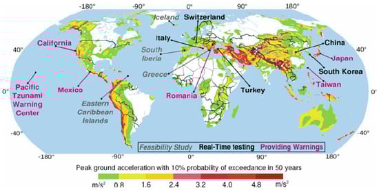
Figure 1. The map shows Earthquakes Early Warning Systems around the world.

Within this framework, it is important to highlight that in recent years, considerable emphasis has been placed on the advancement of diverse models for the early detection of seismic events, which have become available to the wider public through mobile applications, television broadcasts, and radio communication [13]. The primary function of Android applications is that, once an earthquake is detected, an alert is transmitted to all smartphones located within the affected area. Provided that the user is not in close proximity to the epicenter, the notification can be received in advance, allowing sufficient time to take protective action before the destructive seismic waves arrive [14,15,16,17]. By harnessing technology as an ally against natural disasters, humanity can move beyond the devastating consequences of major earthquakes, such as the 2004 Indian Ocean event with more than 220,000 fatalities, the 2011 Tōhoku earthquake in Japan with over 19,000 losses, and the 2023 Turkey–Syria earthquake with more than 43,000 deaths. Accordingly, resilience and sustainability for populations affected by seismic events encompass both physical and social infrastructures capable of withstanding earthquakes, while simultaneously safeguarding long-term well-being through disaster risk reduction, community preparedness, and equitable recovery.

Subsequently, we will proceed with the presentation of related studies alongside our own, which progressively enhance both our sustainability and our capacity for prevention against seismic phenomena. Housner, in 1964, concluded that artificial earthquakes constitute adequate representations of strong-motion events for structural analysis and may serve as standard ground motions in the design of engineering structures [18]. Adeli, in 2009, proposed a novel feature extraction technique, asserting that when combined with a selected Probabilistic Neural Network (PNN), it can yield reliable prediction outcomes for earthquakes with magnitudes ranging from 4.5 to 6.0 on the Richter scale [19]. Zhou, in 2012, introduced a robust feature extraction approach, the Log-Sigmoid Frequency Cepstral Coefficients (LSFCCs), derived from the Mel Frequency Cepstral Coefficients (MFCCs), for the classification of ground targets using geophones. Employing LSFCCs, the average classification accuracy for tracked and wheeled vehicles exceeds 89% across three distinct geographical settings, achieved with a single classifier trained in only one of these environments [20]. Martinez-Alvarez, in 2013, investigated the utilization of various seismicity indicators as inputs for artificial neural networks. The study proposes combining multiple indicators—previously shown to be effective across different seismic regions through the application of feature selection techniques [21]. Schmidt, in 2015, proposed an efficient and automated method for seismic feature extraction. The central concept of this approach is to interpret a two-dimensional seismic image as a function defined on the vertices of a carefully constructed underlying graph [22]. Narayanakumar, in 2016, extracted seismic features from a predetermined number of events preceding the main shock in order to perform earthquake prediction using the backpropagation (BP) neural network technique [23]. Cortes, in 2016, sought to identify the parameters most effective for earthquake prediction. As various studies have employed different feature sets, the optimal selection of features appears to depend on the specific dataset used in constructing the model [24]. Asim, in 2018, developed a hybrid embedded feature selection approach designed to enhance the accuracy of earthquake prediction [25]. Chamberlain, in 2018, demonstrated that synthetic seismograms, when applied with matched-filter techniques, enable the detection of earthquakes even with limited prior knowledge of the source [26]. Okada, in 2018, employed observational data either by calibrating parameters within existing models or by deriving models and indicators directly from the data itself [27]. Lin, in 2018, employed the earthquake catalogue from 2000 to 2010, comprising events with a Richter magnitude (ML) of 5 and a depth of 300 km within the study area (21–26° N, 119–123° E). This dataset was utilized as training input to develop the initial earthquake magnitude prediction backpropagation neural network (IEMPBPNN) model, which was designed with two hidden layers [28]. Zhang, in 2019, proposed a precursory pattern-based feature extraction approach aimed at improving earthquake prediction performance. In this method, raw seismic data are initially segmented into fixed daily time intervals, with the magnitude of the largest earthquake within each interval designated as the main shock [29]. Rohas’s, in 2019, paper reviewed the latest uses of artificial neural networks for automated seismic data interpretation, focusing especially on earthquake detection and onset-time estimation [30]. Ali, in 2020, generated synthetic seismic data for a three-layer geological model and analyzed using Continuous Wavelet Transform (CWT) to identify seismic reflections in both the temporal and spatial domains [31]. Bamer, in 2021, demonstrated, through comparison with several state-of-the-art studies, that the convolutional neural network autonomously learns to extract pertinent input features and structural response behavior directly from complete time histories, rather than relying on a predefined set of manually selected intensity measures [32]. Wang, in 2023, reports that the accuracies of various AI models using the feature extraction dataset surpassed those obtained with the spectral amplitude dataset, demonstrating that the feature extraction approach more effectively emphasizes the distinctions among different types of seismic events [33]. Ozkaya, in 2024, developed a novel feature engineering framework that integrates the Butterfly Pattern (BFPat), statistical measures, and wavelet packet decomposition (WPD) functions. The proposed model achieved an accuracy of 99.58% in earthquake detection and 93.13% in three-class wave classification [34]. Sinha’s review, in 2025, offers valuable insights into cutting-edge techniques and emerging directions in feature engineering for seismic prediction, highlighting the importance of interdisciplinary collaboration in advancing earthquake forecasting and reducing seismic risk [35]. Mahmoud, in 2025, investigates the application of machine learning approaches to earthquake classification and prediction using synthetic seismic datasets [36].

In contrast to the aforementioned studies, this paper introduces a novel approach constructing artificial features with Grammatical Evolution [37] for earthquake prediction, marking the first application of this evolutionary technique in the field of seismology. While the method does not directly address a specific gap in the literature, the experiments demonstrated that feature construction achieved an overall accuracy of 91%, thereby contributing to the advancement of earthquake prediction research. We consider this contribution significant in enhancing the understanding of seismic phenomena and in highlighting the potential of Grammatical Evolution as a promising tool for feature engineering in geophysical datasets. In particular, the method of Grammatical Evolution can be considered as a genetic algorithm [38] with integer chromosomes. Each chromosome contains a series of production rules from the provided Backus–Naur form (BNF) grammar [39] of the underlying language, and hence, this method can create programs that belong to this language. This procedure has been used with success in various cases, such as data fitting problems [40,41], problems that appear in economics [42], computer security problems [43], problems related to water quality [44], problems appearing in medicine [45], evolutionary computation [46], hardware issues in data centers [47], solutions of trigonometric problems [48], automatic composition of music [49], dynamic construction of neural networks [50,51], automatic construction of constant numbers [52], playing video games [53,54], problems regarding energy [55], combinatorial optimization [56], security issues [57], automatic construction of decision trees [58], problems in electronics [59], automatic construction of bounds for neural networks [60], construction of Radial Basis Function networks [61], etc. This research work focuses on the creation of artificial features from existing ones, aiming at two goals: on the one hand, it seeks to reduce the information required for the correct classification of seismic data, and on the other hand, it seeks to highlight the hidden non-linear correlations that may exist between the existing features of the objective problem. In this way, a significant improvement in the classification of seismic data will be achieved.

Beyond the Grammatical Evolution approach proposed in this study, which achieved an accuracy of 91%, we also provide a concise comparison with results from related research that has employed alternative machine learning techniques in the field of seismology. In the study by Adeli et al. [19], the PNN model demonstrated satisfactory predictive accuracy for earthquakes with magnitudes between 4.5 and 6.0, but its performance declined considerably for events exceeding a magnitude of 6.0. Zhou et al. [20] reported that the application of the Log-Sigmoid Frequency Cepstral Coefficient method achieved an average classification accuracy exceeding 89%. Narayanakumar et al. [23] investigated the prediction of moderate earthquakes (magnitude 3.0–5.8). While the seismometer recorded an event of magnitude 4.0, the BP-ANN model predicted magnitudes in the range of 3.0–5.0, achieving a success rate between 75% and 125%. According to Asim et al. [25], the SVR-HNN prediction model achieved its highest performance in Southern California, with MCC, R score, and accuracy values of 0.722, 0.623, and 90.6%, respectively. The Chilean region ranked second, yielding an MCC of 0.613, an R score of 0.603, and an accuracy of 84.9%. In contrast, the Hindukush region exhibited the lowest performance, with MCC, R score, and accuracy values of 0.600, 0.580, and 82.7%, respectively. Chamberlain et al. [26] reported that template-based detections produced 7340 events, of which 3577 were identified as duplicates, whereas the STA/LTA method yielded 682 detections over the same time interval. Lin et al. [28] reported that the average magnitude error in Taiwan was $\Delta ML=\pm 0.3$, while the training errors of the EEMPBPNN model (<0.25) remained below this average error threshold. Zhang et al. [29] demonstrated that the proposed method achieved prediction accuracies of 93.26% and 92.07% across the two datasets examined. Rojas et al. [30] reported recognition performance of approximately 99.2% for P-wave signals and 98.4% for pure noise. Ali et al. [31] conducted a statistical analysis using a 95% confidence interval for the normalized CWT coefficients of P-wave velocity, seismic trace, acoustic impedance, and synthetic seismic trace. Wang et al. [33] found that, in the model generalization evaluation, the two-class models trained on the 36-dimensional network-averaged dataset achieved test accuracies and F1 scores exceeding 90%. Ozkaya et al. [34] reported that their model achieved an accuracy of 99.58% in earthquake detection and 93.13% in three-class wave classification. While comparable studies have demonstrated strong performance, many of them are limited to specific regions of interest or focus on particular signal types, such as acoustic wave detection. In contrast, the Grammatical Evolution approach presented here not only achieves competitive accuracy (91%) but also demonstrates broader applicability across diverse seismic datasets, thereby highlighting its potential as a more generalizable solution in earthquake event discrimination.

The rest of this manuscript is organized as follows: The used dataset and the incorporated methods used in the conducted experiments are outlined in Section 2, the experimental results are shown and discussed in Section 3, and finally, a detailed discussion is provided in Section 4.

2. Materialsand Methods

In this section, a detailed presentation of the datasets used as well as the machine learning techniques used in the experiments performed will be provided.

2.1. The Dataset Employed

In this study, we made use of open data from the NSF Seismological Facility for the Earth Consortium (SAGE) available from https://ds.iris.edu/ (accessed on 25 November 2025), which is a platform offering an interactive global map that facilitates both data visualization and the real-time extraction of datasets from the displayed geographic regions. The area defined by latitudes 33–44° and longitudes 17–44° covers 28 seismic zones, with Turkey and Greece identified as the most seismically active regions.

Regarding the 28 seismic zones listed in Table 1, these correspond to specific geographic coordinates (latitudes and longitudes) provided through the interactive seismic platform previously referenced. The platform grants direct access to these spatial data, ensuring that the delineation of the zones is both systematic and consistent with the established geospatial framework.

Table 1. Regions codes for the 28 seismic zones.

Region	Region Code
Turkey	1
Crete Greece	2
Greece	3
Dodecanese Islands, GREECE	4
Ionian Sea	5
Aegean Sea	6
Southern Greece	7
GREECEALBANIA border region	8
GREECEBULGARIA border region	9
Cyprus region	10
Albania	11
NORTHWESTERN Balkan Region	12
Central Mediterranean sea	13
Jordan Syria region	14
GEORGIA ARMENIA TURKEY	15
Border Region
TURKEY IRAN border region	16
Iraq	17
Eastern Mediterranean sea	18
NORTHWESTERN CAUCASUS	19
Black Sea	20
Romania	21
Bulgaria	22
Crimea Region Ukraine	23
ARMENIA AZERBAIJAN IRAN	24
border region
Adriatic sea	25
UKRAINE MOLDOVA RUSSIA	26
border region
Southern Italy	27
IRAN IRAQ border region	28

Furthermore, the selection of NSF data was driven by its advanced functionality and broad accessibility. Notably, it supports the download of up to 25,000 records per file, thereby streamlining the workflow and improving the efficiency of information retrieval. The region under investigation is presented in Figure 2. This image was retrieved from IRIS Earthquake Browser, in the following URL: https://ds.iris.edu/ieb/index.html?format=text&nodata=404&starttime=2010-01-01&endtime=2010-12-31&orderby=time-desc&src=iris&limit=1000&maxlat=74.85&minlat=-7.26&maxlon=135.19&minlon=-97.36&zm=3&mt=ter (accessed on 7 January 2026).

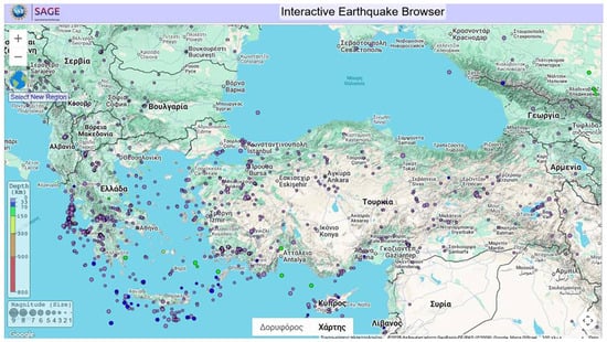
Figure 2. The study area.

2.2. Dataset Description

We obtained and systematically analyzed 511,064 earthquake events from 1990 to 2015, as this time period is of particular scientific interest due to the surge in seismic activity, as also illustrated in the graph of Figure 3. Specifically, we selected this time period because it encompasses a wide range of earthquake magnitudes, which provides a diverse dataset conducive to algorithm training and supports the construction of artificial features via Grammatical Evolution.

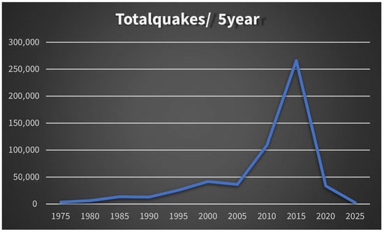
Figure 3. Graphs of seismic events from 1970 to 2025 (study area).

In the years under examination, earthquakes are distributed across all magnitude classes, exhibiting an almost ideal proportion consistent with the Gutenberg–Richter law [62]. For instance, within the first two five-year periods of our dataset, 2 events above magnitude 8.0, 3 events above magnitude 7.0, 19 events above magnitude 6.0, 165 events between 5.0 and 5.9, 3048 events between 4.0 and 4.9, and 26,301 events between 3.0 and 3.9 were recorded, thereby confirming the expected logarithmic relationship between frequency and magnitude. Such a balanced and representative dataset further enhances the effectiveness of the Grammatical Evolution approach, as it provides a comprehensive distribution of seismic events across the full spectrum of magnitudes. Moreover, our analysis led us to the conclusion that the datasets from 1970 to 1989 and 2016 to 2025 lack the diversity observed in the dataset we selected. Specifically, classes 6 and 7 are entirely absent from the 1970–1989 records, while in the post-2016 data, class 7 is missing and class 1 contains only a limited number of instances, namely 25.

On the platform that provides us with the Interactive Earthquake Browser, we employed coordinates spanning latitudes 33–44° and longitudes 17–44°, considered magnitude values from 1.0 to 10.0, and incorporated all available depths by default within the depth range. The raw dataset included the following variables: year, month, day, time, latitude (Lat), longitude (Lon), depth, magnitude, region, and timestamp. Accordingly, Table 2 provides a detailed overview of the raw dataset.

Table 2. Raw data from NSF Interactive Earthquake Browser (1990–2015).

Raw Data
Features	Range
Year	1990–2015
Month	1–12
Day	1–31
Time	00:00:00–23:59:59
Latitude	33–44
Longitude	17–44
Region	1–28
Depth	0.00–800.00
Magnitude	1–10
Timestamp

Subsequently, a preprocessing procedure was applied to the dataset. This included the identification of the lithospheric plate associated with each earthquake, to which a unique code was assigned. Furthermore, the months were categorized according to the four seasons, the days were grouped into ten-day intervals, and the time of occurrence was classified into four periods (morning, noon, afternoon, and night). The focal depth was divided into six categories. In addition, a new column was created to indicate, with a binary value (0 or 1), whether an earthquake had previously occurred in the same region during the same season. Finally, the dataset was merged with the Kp index, representing geomagnetic storm activity, which was further classified into six distinct categories. The final dataset was further processed, including the following: Year, Epoch Code, Day Code, Time Code, Latitude, Longitude, Depth Code, Previous Magnitude Code, Same Region Code, Lithospheric/Tectonic Plate, Kp Code. This information is outlined in Table 3.

Table 3. Utilized data from NSF Interactive Earthquake Browser (1990–2015).

Utilized Data
Features	Range	Class
Year	1990–2015
Epoch Code	1–12	0–3
Day Code	1–31	0–2
Time Code	00:00:00–23:59:59	0–3
Latitude	33–44
Longitude	17–44
Depth Code	0.00–800.00	0–5
Previous Magnitude Code	1–10	1–7
Same Region Code	1–28	1–28
Lithospheric Code	1–7	1–7
Kp Code	0.000–9.000	0–5

In the processed dataset, categorical classes were introduced to facilitate the analysis. Specifically, the months were initially ordered numerically and subsequently grouped according to the corresponding season. Thus, class 0 represents the winter months, class 1 corresponds to the spring months, class 2 to the summer months, and class 3 to the autumn months. The days comprising each month were divided into three ten-day intervals, with the first interval assigned to class 0, the second interval to class 1, and the final interval to class 2. Accordingly, the hours of the 24 h day were divided into distinct periods, with the morning zone assigned to class 0, midday to class 1, afternoon to class 2, and night to class 3. For the depth code, earthquakes occurring near the surface (0–32.9 km) were assigned to class 0, those recorded at depths between 33 and 69.9 km to class 1, events within 70–149.9 km to class 2, those between 150 and 299.9 km to class 3, earthquakes at depths of 300–499.9 km to class 4, those between 500 and 799.9 km to class 5, and finally, events occurring at depths greater than 800 km were assigned to class 6. Continuing, earthquakes with magnitudes below 2.9 were assigned to class 1, those with magnitudes between 3.0 and 3.9 to class 2, magnitudes between 4.0 and 4.9 to class 3, magnitudes between 5.0 and 5.9 to class 4, magnitudes between 6.0 and 6.9 to class 5, magnitudes between 7.0 and 7.9 to class 6, while events with magnitudes of 8.0 and above were assigned to class 7. With regard to the categorization of the geographical region and the lithospheric plate, each region was assigned a code ranging from 1 to 28. Similarly, a code from 1 to 7 was allocated to the lithospheric plates corresponding to each seismic event. Finally, the Kp code was classified as follows: values ranging from 0.000 to 4.000 were assigned to class 0, those from 4.100 to 5.000 to class 1, values between 5.100 and 6.000 to class 2, those from 6.100 to 7.000 to class 3, values between 7.100 and 8.000 to class 4, and finally, values from 8.100 to 9.000 were assigned to class 5.

At the following stage of data processing, we elected to focus on earthquakes with a magnitude code of 2 and above, since the inclusion of lower-magnitude events would bias the model toward predicting minor seismic occurrences. Notably, the small-magnitude category (1–2.9 mag) prevailed as the majority class with 407,144 records, creating a significant imbalance in the dataset. By excluding this dominant class, we aimed to achieve a more balanced distribution across magnitudes and to enhance the representational capacity of the model. This approach is consistent with previous studies that have similarly excluded small earthquakes to mitigate bias and improve predictive performance. Wang et al., in 2023, reports in Dataset and Feature Engineering “The seismic catalog used in this study was obtained from the China Earthquake Data Center (CEDC, http://data.earthquake.cn/, last accessed on 12 December 2025) and includes earthquake events with a magnitude greater than 3.0 in the Sichuan-Yunnan region from 1970 to 2021” [63]. It is noteworthy that the division into two classes within the field of seismology has previously been employed, as in the study of Zhang et al. (2023), which investigated seismic data by categorizing events into high magnitude ($M\ge 5.5$) and low magnitude ($M<5.5$) [64]. Following these steps, we proceeded with our experiments, utilizing approximately 10,000 seismic events in order to generate artificial features through Grammatical Evolution.

In summary, the seismic data employed in this study were recorded on the magnitude scale, covering events from 1 to 10. Initially, we excluded small earthquakes, which predominated in number and affected the balance of the dataset. The data source was the EarthScope Consortium, which operates the NSF Geodetic Facility for the Advancement of Geoscience (GAGE) and the NSF Seismological Facility for the Advancement of Geoscience (SAGE). These records were obtained from thousands of stations worldwide, constituting the primary NSF SAGE archive.

2.3. Global Optimization Methods for Neural Network Training

In the current work, two well-known global optimization methods were incorporated for neural network training [65,66], the Genetic Algorithm and the Particle Swarm Optimization (PSO) method. The Genetic Algorithm is an evolutionary optimization method designed to minimize an objective function defined over a continuous search space. It operates on a population of candidate solutions, each represented as a vector of parameters, and this population evolves through a series of steps, where in each step, some processes that resemble natural processes are applied to the population. Genetic Algorithms have applied on a wide range of applications that include training of neural networks [67,68]. Beyond neural network training, Genetic Algorithms have demonstrated strong performance in physics, biotechnology, and medical physics. In bioinformatics and biotechnology, they are commonly applied to the analysis of biological data, gene selection, and the optimization of complex biological systems [69]. In medical physics and biomedical engineering, GAs have been successfully used for medical image segmentation [70], diagnostic modeling, and the optimization of treatment parameters [71]. They have also been applied to multi-objective problems related to energy efficiency, economic viability, environmental life-cycle assessment [72], and parameter identification in complex multi-physics energy systems [73]. Also, Figure 4 presents the basic steps of a Genetic Algorithm.

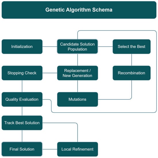
Figure 4. The main steps of the Genetic Algorithm.

Particle Swarm Optimization (PSO) is a population-based search method inspired by how animals move and cooperate in groups like flocks of birds or schools of fish [74,75]. The PSO was widely used in a variety of practical problems as well as in neural network training [76,77]. Beyond neural network training, Particle Swarm Optimization has been applied across a broad spectrum of scientific and technological domains. In particular, it has found significant use in economic and resource optimization [78], as well as in healthcare management and medical physics, where it supports efficient medical service allocation and the management of stochastic patient queue systems [79]. At the same time, PSO has been increasingly adopted in physics and chemical engineering for the optimization of catalytic processes and energy systems, often in combination with deep learning approaches to extract meaningful physical and chemical insights [80]. In more dynamic and decentralized settings, PSO has proven especially effective in robotics, where it is used to coordinate swarms of autonomous robots during search-and-rescue missions operating under uncertain and rapidly changing conditions [81]. Finally, its flexibility has also led to successful applications in bioinformatics and computational biology, where advanced multi-objective PSO variants are employed for community detection and the identification of disease-related functional modules within complex biological networks [82]. The main steps of the PSO method are outlined in Figure 5.

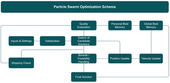
Figure 5. The main steps of the PSO algorithm.

2.4. The SVM Method

The Support Vector Machine (SVM) is a supervised learning algorithm applied to both classification and regression problems [83]. The concept of Support Vector methods was introduced by V. Vapnik in 1965, in the context of addressing challenges in pattern recognition. During the 1990s, V. Vapnik formally introduced Support Vector Machine (SVM) methods within the framework of Statistical Learning. Since their introduction, SVMs have been extensively employed across diverse domains, including pattern recognition, natural language processing, and related applications [84]. For instance, the SVM algorithm has been employed both in studies on earthquake prediction and in research on the early detection of seismic phenomena, as demonstrated in the following works: Hybrid Technique Using Singular Value Decomposition (SVD) and Support Vector Machine (SVM) Approach for Earthquake Prediction [85], Using Support Vector Machine (SVM) with GPS Ionospheric TEC Estimations to Potentially Predict Earthquake Events [86], The efficacy of Support Vector Machines (SVM) in robust determination of earthquake early warning magnitudes in central Japan [87]. As with other comparative analyses of models, SVMs require greater computational resources during training and exhibit reduced susceptibility to overfitting, whereas neural networks are generally regarded as more adaptable and capable of scaling effectively. Beyond these applications, SVMs have also been widely adopted in several applied scientific and engineering fields. In bioinformatics, SVMs are commonly employed to analyze and interpret complex biological data, where their ability to handle high-dimensional feature spaces is particularly valuable [88]. In medical imaging and clinical applications, they have been used effectively for disease classification and staging, such as the prediction of lung cancer stages from medical imaging data [89]. In addition, SVM-based models are increasingly integrated into healthcare monitoring systems, including Internet of Medical Things (IoMT) frameworks, where reliability and robustness are critical requirements [90]. Moreover, SVMs have been applied in applied physics and engineering, including the prediction of electronic properties in advanced material structures and nanocomposites [91]. Their robustness has also made them suitable for safety-critical applications, such as fault detection and diagnosis in nuclear power plant systems [92].

2.5. The Neural Network Construction Method

Another method used in the experiments to predict the category of seismic vibrations is the method of constructing artificial neural networks using Grammatical Evolution [93]. This method can detect the optimal architecture for neural networks as well as the optimal set of values for the corresponding parameters. This method was used in various cases, such as chemistry problems [94], solution of differential equations [95], medical problems [96], educational problems [97], detection of autism [98], etc. This method can produce neural networks in the following form:

$$N\left(\overrightarrow{x},\overrightarrow{w}\right)=\sum _{i=1}^H{w}_{(d+2)i-(d+1)}\sigma \left(\sum _{j=1}^d{x}_j{w}_{(d+2)i-(d+1)+j}+w_{(d+2)i}\right)$$

(1)

In this equation, the value H represents the number of used computation units (weights) for the neural network. The vector w denotes the vector containing the parameters of the neural network and vector x represents the input vector (pattern). The function $\sigma \left(x\right)$ stands for the sigmoid function, which is defined as

$$\sigma \left(x\right)={\displaystyle \frac{1}{1+exp(-x)}}$$

(2)

2.6. The Proposed Method

The method proposed here to tackle the classification of seismic events is a procedure that constructs artificial features from the original ones using Grammatical Evolution. The method was initially presented in the paper of Gavrilis et al. [99] and used in various cases in the past [100,101,102]. The main steps of this method have as follows:

• Initialization step.

  (a)

  Obtain the training data and denote them using the M pairs $\left(x_i,t_i\right),i=1\dots M$. The values $t_i$ represent the actual output for the input pattern $x_i$.

  (b)

  Set the parameters of the used genetic algorithm: $N_g$ for the number of allowed generations,  $N_c$  for the number of chromosomes, $p_s$  for the selection rate, and  $p_m$  for the mutation rate.

  (c)

  Set as $N_f$ the number of artificial features that will construct the current method.

  (d)

  Initialize every chromosome $g_i,i=1,\dots ,N_g$ as a set of randomly selected integers.

  (e)

  Set $k=1$, the generation counter.

• Genetic step.

  (a)

  For $i=1,\dots ,N_g$ do

  • Construct with Grammatical Evolution a set of $N_f$ artificial features for each chromosome $g_i$. The BNF grammar used for this procedure is shown in Figure 6.
    

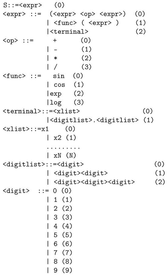    Figure 6. The grammar used for the proposed method. The numbers in parentheses indicate the increasing number of the production rule for the corresponding non-terminal symbol.
  • Transform the original set of features using the constructed features and denote the new training set as $\left(x_{g_i,j},t_j\right),j=1,\dots M$.
  • Train a machine learning C on the new training set. The training error for this model will represent the fitness $f_i$ for the current chromosome, and it is computed as

    $$f_i=\sum _{j=1}^M{\left(C\left(x_{g_i,j}\right)-t_j\right)}^2$$

    (3)
    In the current work, the Radial Basis Function networks (RBF) [103,104] were used as the machine learning models. A decisive factor for this choice was the short training time required for these machine learning models.
  • Perform the selection procedure: Initially, the chromosomes are sorted according to the associated fitness values and the best $\left(1-p_s\right)\times N_C$ of them are copied intact to the next generation. The remaining chromosomes will be replaced by offsprings that will be produced during the crossover and the mutation procedure.
  • Perform the crossover procedure: The outcome of this process is a set of $p_s\times N_c$ new chromosomes. For every pair $\left(\tilde{z},\tilde{w}\right)$ of new chromosomes, two distinct chromosomes z and w are chosen from the current population using the process of tournament selection. Afterwards, the new chromosomes are produced using the procedure of one-point crossover, which is illustrated in Figure 7.
    

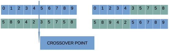    Figure 7. An example of the one-point crossover method. The blue color denotes the first chromosome and the green color the parts of the second chromosome.
  • Execute the mutation procedure: During this procedure a random number $r\in \left[0,1\right]$ is selected for each element of every chromosome. The corresponding element is altered randomly if $r\le p_m$.

  (b)

  EndFor

• Set $k=k+1$.
• If $k\le N_g$ go to Genetic Step.
• Obtain the best chromosome $g^{\ast }$ from the current population.
• Create the corresponding $N_f$ features for $g^{\ast }$ and apply these features to the set and report the corresponding test error.

Also, a flowchart that presents the overall process of feature construction is presented in Figure 8.

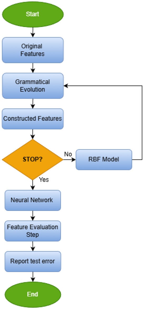
Figure 8. The steps of the feature construction procedure.

Moreover, a graphical pipeline that summarizes the whole procedure is depicted in Figure 9.

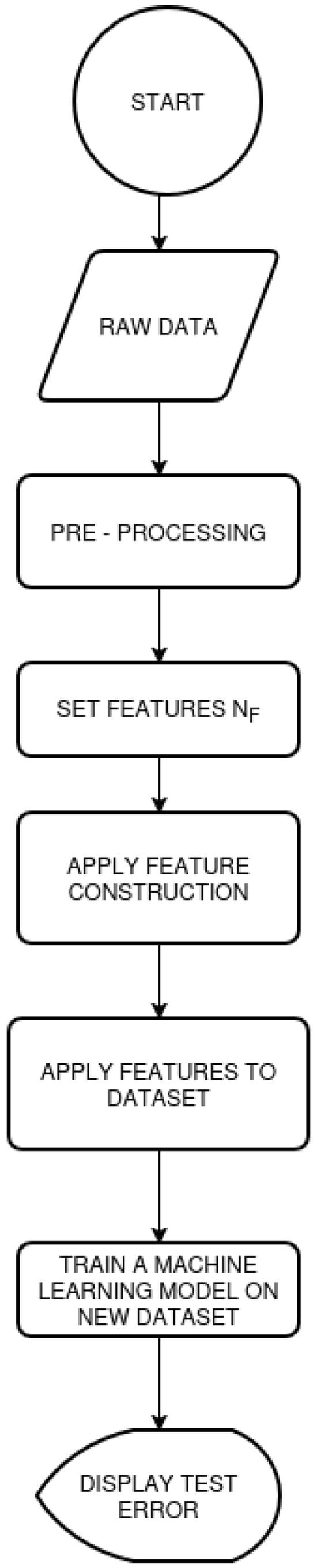
Figure 9. The pipeline of the used procedure.

3. Results

The methods used in the conducted experiments were coded in ANSI C++, with the assistance of the freely available optimization package of OPTIMUS [105]. Moreover, for the feature construction procedure, the freely available programming tool QFc, which can be downloaded from https://github.com/itsoulos/QFc (accessed on 12 December 2025) [106] was used. Each experiment was conducted 30 times, using different seeds for the random generator in each execution. Also, the procedure of ten-fold cross-validation was incorporated to validate the conducted experiments. The values for the experimental parameters are listed in Table 4. The parameters in this table have been chosen to provide a compromise between speed and efficiency of the proposed procedure and were applied to all methods used in the experiments, so that there is fairness in the comparison of experimental results. The proposed method of feature construction was applied to each individual fold and averages of the classification errors in the control sets were obtained. In addition, the RBF machine learning model was used to construct the new features due to the significantly shorter learning time required for it compared to other models, such as artificial neural networks.

Table 4. The values of the experimental parameters.

Parameter	Meaning	Value
$N_g$	Number of generations	500
$N_c$	Number of chromosomes	500
$p_s$	Selection rate	0.9
$p_m$	Mutation rate	0.05
$N_f$	Number of features	2

Table 5 reports the classification error rates for five temporal subsets of the seismic dataset (GCT1990, GCT1995, GCT2000, GCT2005, GCT2010), where the first column encodes the year of the data and the remaining columns correspond to the machine learning models MLP(GEN), MLP(PSO), SVM, NNC, and the proposed FC (future construction) model. The values are expressed as percentage classification errors, that is, the proportion of misclassified events between the two seismic classes defined during preprocessing (events with magnitude code 2–3 versus events with a magnitude greater than 3). The following notation is used in this table:

Table 5. Experimental results using a series of machine learning methods.

DATASET	MLP(GEN)	MLP(PSO)	SVM	NNC	FC
GCT1990	39.98%	38.21%	14.30%	22.72%	13.50%
GCT1995	38.08%	33.22%	13.48%	21.50%	10.82%
GCT2000	26.70%	27.48%	10.19%	24.59%	6.52%
GCT2005	38.44%	33.19%	6.85%	27.85%	4.45%
GCT2010	52.89%	44.77%	14.46%	29.81%	9.97%
AVERAGE	39.22%	35.37%	11.86%	25.29%	9.05%

• The column MLP(GEN) denotes the error from the application of the Genetic Algorithm described in Section 2.3 for the training of a neural network with 10 processing nodes.
• The column MLP(PSO) represents the incorporation of the PSO method given in Section 2.3 for the training of a neural network with 10 processing nodes.
• The column SVM represents the application of the SVM method, described in Section 2.4. In the current implementation, the freely available library LibSvm [107] was used.
• The column NNC represents the neural network construction method, described in Section 2.5.
• The column FC denotes the proposed feature construction technique, outlined in Section 2.6.
• The row AVERAGE denotes the average classification error for all datasets.

Also, Table 6 indicates the precision and recall values for SVM, NNC, and the proposed method.

Table 6. Precision and recall values for the methods SVM, NNC, and FC.

	SVM		NNC		FC
DATASET	PRECISION	RECALL	PRECISION	RECALL	PRECISION	RECALL
GCT1990	0.798	0.837	0.684	0.728	0.800	0.874
GCT1995	0.811	0.830	0.684	0.729	0.801	0.886
GCT2000	0.835	0.844	0.662	0.700	0.835	0.901
GCT2005	0.856	0.869	0.628	0.627	0.856	0.904
GCT2010	0.802	0.824	0.633	0.628	0.804	0.805

The most striking observation is that FC achieves the lowest error for all five datasets, with no exceptions. For every GCT year, the FC column attains the minimum error among all models, demonstrating a consistent and temporally robust superiority. This pattern is clearly reflected in the AVERAGE row: the mean classification error of FC is 9.05%, whereas the corresponding mean error of the best conventional baseline, the SVM, is 11.86%. Moving from 11.86% to 9.05% corresponds to an error reduction of approximately 24–25%, meaning that roughly one quarter of the misclassifications made by the SVM are eliminated when using FC. Compared with the neural approaches, the gain is even more pronounced: FC reduces the mean error from 39.22% to 9.05% for MLP(GEN), from 35.37% to 9.05% for MLP(PSO), and from 25.29% to 9.05% for NNC, effectively absorbing about 64–77% of their errors.

Examining the behaviour per year reveals how the proposed model interacts with the specific characteristics of each temporal subset. Dataset GCT2005 appears to be the “easiest” case for all models, with the SVM dropping to 6.85% error and FC reaching 4.45%, which corresponds to an accuracy of about 95.5%. At the opposite end of the spectrum, GCT2010 is clearly the most challenging dataset, as indicated by substantially increased errors for the conventional models (MLP(GEN) 52.89%, MLP(PSO) 44.77%, NNC 29.81%) and by a higher error for the SVM (14.46%). Even in this difficult scenario, FC keeps the error below 10% (9.97%), preserving a clear qualitative advantage in the most demanding temporal setting. A similar pattern emerges for the intermediate years 1995 and 2000, where FC-SVM absolute differences are in the range of 2–4 percentage points, corresponding to roughly 20–35% relative error reduction. This suggests that as the data become more complex, the benefit of the automatically constructed features generated by Grammatical Evolution becomes increasingly pronounced.

A second important finding is that the ranking of the conventional models remains stable across all years. The SVM is consistently the best among the standard baselines, followed by NNC and the two MLP variants, with MLP(PSO) systematically outperforming MLP(GEN). This stability reinforces the credibility of the table as a benchmark, indicating that the results are not driven by noise or random fluctuations but instead reflect a coherent hierarchy of model performance. On top of this stable baseline, FC does not merely swap the winner for a single dataset, it establishes a new performance level by consistently pushing the error rates to substantially lower values in every year.

From a practical standpoint, given that the final processed dataset contains on the order of 10,000 seismic events, an average error of 11.86% compared with 9.05% implies hundreds of fewer misclassified instances when FC is used instead of a plain SVM trained on the original features. This has direct implications for early warning and risk assessment applications, where each reduction in misclassification translates into more reliable decision-making. The evidence from Table 5, combined with the methodological description, strongly supports the view that the feature construction phase based on Grammatical Evolution is not a minor refinement over existing classifiers, but rather a key component that reshapes the feature space so that the seismic classes become much more separable. This explains why the proposed FC model achieves an average error of approximately 9%, in full agreement with the reported overall accuracy of 91% in the abstract.

Overall, Table 6 shows that FC is not only the best-performing model in each individual year but also the most stable across different temporal subsets, confirming that the future construction approach with Grammatical Evolution yields a substantial and consistent improvement over standard machine learning models for the discrimination of seismic events.

The repeated-measures ANOVA with Method as the within-subject factor and DATASET (year) as the blocking factor confirms that the choice of classifier has a statistically significant effect on the classification error, indicating that the models are not equivalent in terms of predictive performance. Building on this global result, we conducted pairwise paired t-tests between the proposed FC model and each baseline, using one-sided alternatives that explicitly test the hypothesis that FC achieves lower mean error than its competitors. The resulting p-values, visualized as significance stars on the boxplot, show that the superiority of FC is statistically supported across all comparisons (Figure 10).

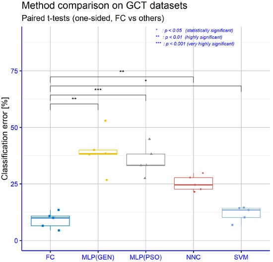
Figure 10. Comparison of FC and baseline classifiers on GCT datasets (paired one-sided t-tests on classification error).

In particular, the comparisons of FC vs. MLP(GEN) and FC vs. NNC yield ** (p < 0.01), indicating that the probability of observing differences of this magnitude in favor of FC purely by chance is below 1%. An even stronger effect emerges for FC vs. MLP(PSO), which is marked with *** (p < 0.001), reflecting the very large performance gap between FC and the PSO-trained MLP. Finally, the comparison of FC vs. SVM is annotated with * (p < 0.05), showing that, although the numerical difference in error is smaller than in the neural baselines, it remains statistically significant in favor of FC. Overall, the pattern of significance codes (*, **, ***) corroborates the message of Table 6: FC is not only the best-performing model in terms of average classification error, but its advantage over all other methods is statistically significant, with particularly strong evidence against the MLP-based models and clear, though more moderate, evidence against the already very competitive SVM baseline.

Also, a graphical summary that graphically represents the comparison between the different machine learning methods is depicted in Figure 11.

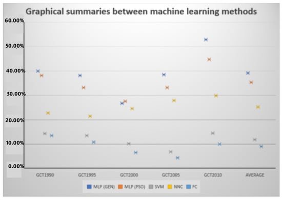
Figure 11. Graphical comparison of the used machine learning methods.

Moreover, the proposed method can identify the hidden relationships between the features of the objective dataset. As an example of constructed features, consider the following two features created for a distinct run on the GCT2010 dataset:

$$\begin{array}{ccc}\hfill f_1\left(x\right)& =& sin\left((28.841/9.28)\ast x_{10}+(-78.60)\ast x_3+16.12\ast x_7+6.3\ast x_{11}\right)\hfill \\ \hfill f_2\left(x\right)& =& cos\left(458.6\ast x_2+(-18.809)\ast x_4\right)\hfill \end{array}$$

The following figures provide a concise visual characterization of the artificial features generated by Grammatical Evolution: (i) expression-tree representations for two representative constructed features ($f_1$,$f_2$) and (ii) a complementary summary of the grammar primitives used in these constructions, offering direct insight into both their structural form and their basic building blocks.

Figure 12 (expression tree of $f_1$) visualizes the internal structure of the first constructed feature as an expression tree. The root node corresponds to the non-linear primitive sin, applied to an algebraic core that combines multiple original variables ($x_{10}$, $x_3$, $x_7$, $x_1$) through a weighted sum with constants. This diagram provides an interpretable view of the GE output, indicating that non-linearity is applied over algebraic forms of controlled complexity assembled from grammar primitives.

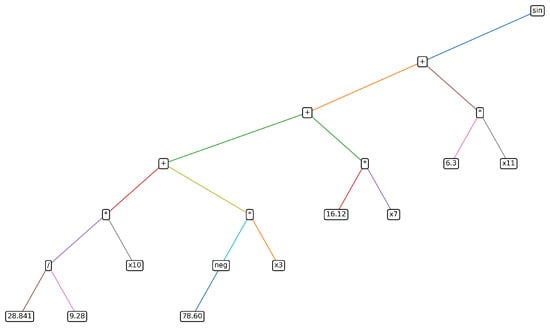
Figure 12. Constructed feature $f_1\left(x\right)$ expression tree. The leaf nodes denote terminal symbols and inner nodes denote non-terminal symbols.

Figure 13 (expression tree of $f_2$) depicts a second constructed feature with a simpler topology: a cos root applied to the sum of two variable terms ($x_2$, $x_4$) with constant coefficients. Compared to $f_1$, this construction has lower structural complexity (fewer nodes/terms) while still introducing non-linearity. The contrast between the two trees illustrates that GE can produce features of varying complexity, ranging from compact to richer expressions, depending on the optimization objective.

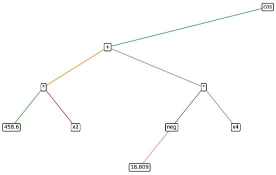
Figure 13. Constructed feature $f_2\left(x\right)$ expression tree. The leaf nodes denote terminal symbols and inner nodes denote non - terminal symbols.

Figure 14 (primitive usage) summarizes the grammar building blocks used in the example constructions ($f_1$,$f_2$), including non-linear functions (sin/cos), arithmetic operators (+, *, /), and terminal variables $x_i$. Bar heights correspond to simple occurrence counts (node counts) of primitives within the two symbolic expressions, while numeric constants are omitted to keep the visualization compact and focused on structural elements. This plot provides an intuitive view of the “vocabulary” employed in these constructions, and the same analysis can be extended by aggregating counts over all runs to describe broader construction trends.

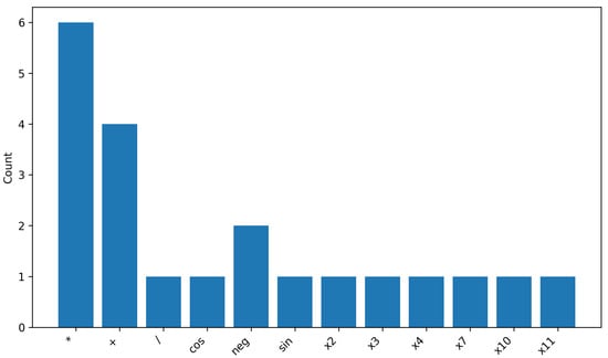
Figure 14. Grammar primitives used in example constructed features ($f_1$, $f_2$).

3.1. Experiments with the Number of Features

An additional experiment was conducted, where the number of constructed features was changed from 1 to 4 for the proposed feature construction method. The corresponding experimental results are outlined in Table 7.

Table 7. Experimental results using the proposed method and a series of values for the number of constructed features $N_f$.

DATASET	${\mathit{N}}_{\mathit{f}}=1$	${\mathit{N}}_{\mathit{f}}=2$	${\mathit{N}}_{\mathit{f}}=3$	${\mathit{N}}_{\mathit{f}}=4$
GCT1990	11.03%	13.50%	14.62%	15.40%
GCT1995	9.41%	10.82%	9.98%	10.05%
GCT2000	6.51%	6.52%	6.75%	6.54%
GCT2005	4.40%	4.45%	4.42%	4.38%
GCT2010	9.72%	9.97%	9.82%	10.32%
AVERAGE	8.21%	9.05%	9.12%	9.34%

Table 7 investigates the behavior of the proposed FC model as the number of constructed features $N_f$ varies from 1 to 4. The results show that performance is generally very stable, with the mean classification error ranging within a narrow band between 8.21% (for $N_f$ = 1) and 9.34% (for $N_f$ = 4). The lowest average error is obtained with a single constructed feature ($N_f$ = 1), whereas the configuration $N_f$ = 2, which is adopted as the default setting in Table 5, yields a mean error of 9.05%, very close to the optimum and with highly consistent behaviour across all years. In some datasets, such as GCT2005, slightly better values appear for larger $N_f$ (e.g., 4.38% for $N_f$ = 4 versus 4.40% for $N_f$ = 1), but these gains are marginal and do not change the overall picture. Taken together, the results indicate that FC does not require a large number of future constructions to perform well: one or two constructed features are sufficient to achieve very low error rates, while further increasing $N_f$ does not lead to systematic improvements and likely introduces redundant information that does not translate into better generalization. This supports the view that the quality of the features generated by Grammatical Evolution is more important than their quantity, and that the proposed choice $N_f$ = 2 offers a well-balanced compromise between performance and model simplicity. Also, Figure 15 presents a comparison for the test error for various cases of the parameter $N_f$.

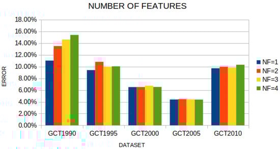
Figure 15. The performance of the proposed method on the used datasets, using various values for the parameter $N_f$.

The boxplot for Table 7, together with the paired t-tests, shows that none of the comparisons among the $N_f$ = 1, $N_f$ = 2, $N_f$ = 3, and $N_f$ = 4 configurations reach statistical significance (all labelled as ns). This indicates that, given the available datasets, the performance of the FC model is essentially insensitive to the number of future constructions, and that using smaller values such as $N_f$ = 1 or $N_f$ = 2 achieves comparable accuracy without any statistically supported gains from increasing $N_f$ (Figure 16).

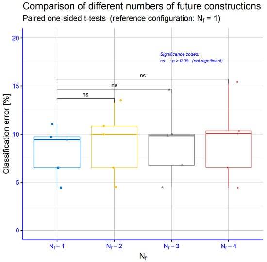
Figure 16. Comparison of FC and baseline classifiers on GCT datasets (paired one-sided t-tests on classification error).

Figure 17 summarizes how the classification error varies with the number of constructed features $N_f$. The left panel plots error versus $N_f$ for each dataset, together with the mean trend (± standard error), indicating that the lowest average error is obtained at $N_f$ = 1. The right panel reports the per-dataset difference $\Delta$ = Error ($N_f$ = k) − Error ($N_f$ = 1) for k ≥ 2, where the dashed line $\Delta$ = 0 corresponds to the $N_f$ = 1 baseline. Predominantly positive $\Delta$ values show that increasing $N_f$ provides no additional benefit and leads to diminishing returns relative to $N_f$ = 1.

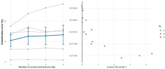
Figure 17. Effect of the number of constructed features $N_f$: consistency of $N_f$ = 1 and diminishing returns.

3.2. Experiments with the Number of Generations

Moreover, in order to test the efficiency of the proposed method, an additional experiment was executed, where the number of generations was altered from 50 to 400.

Table 8 focuses on the number of generations $N_g$ of the evolutionary algorithm during feature construction and evaluates four values (50, 100, 200, 400). The results demonstrate that FC is remarkably robust with respect to this hyperparameter: the mean classification error remains very close across settings, ranging from 9.18% for $N_g$ = 100 down to 8.78% for $N_g$ = 400. The configuration $N_g$ = 200, which is used as the default in the previous analysis, attains an average error of 9.05%, essentially indistinguishable from the more expensive setting $N_g$ = 400, which improves the mean error only by about a quarter of a percentage point. At the level of individual datasets, there are cases where a larger number of generations yields more noticeable gains (for instance, GCT1990 improves to 12.30% at $N_g$ = 400), but the overall pattern is that most of the benefit is already captured within 100–200 generations, with further iterations providing diminishing returns. Thus, Table 8 suggests that the Grammatical Evolution process converges to useful future constructions relatively quickly, and that the choice $N_g$ = 200 offers a very good trade-off between computational cost and predictive performance, avoiding unnecessary increases in training time without delivering substantial accuracy gains. Furthermore, Figure 18 outlines the performance of the proposed method to the used datasets, using different values for the number of generations $N_g.$

Table 8. Experimental results using the proposed method and a series of values for the number of generations $N_g$.

DATASET	${\mathit{N}}_{\mathit{g}}=50$	${\mathit{N}}_{\mathit{g}}=100$	${\mathit{N}}_{\mathit{g}}=200$	${\mathit{N}}_{\mathit{g}}=400$
GCT1990	13.61%	13.19%	13.50%	12.30%
GCT1995	11.06%	11.70%	10.82%	10.74%
GCT2000	6.53%	6.58%	6.52%	6.52%
GCT2005	4.58%	4.45%	4.45%	4.41%
GCT2010	9.88%	10.00%	9.97%	9.94%
AVERAGE	9.13%	9.18%	9.05%	8.78%

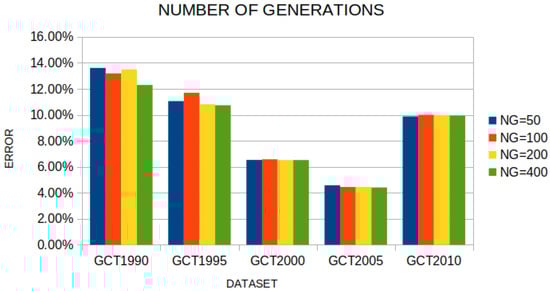
Figure 18. The performance of the proposed method using different values for the parameter $N_g$.

In Figure 19, the paired t-tests for the different numbers of generations show that all pairwise comparisons are non-significant (ns), indicating that variations in $N_g$ do not materially affect the classification error of the FC model.

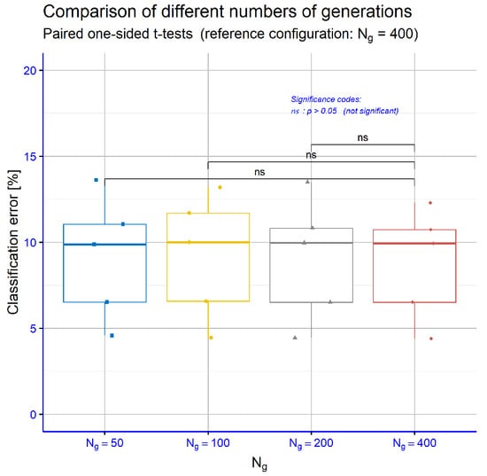
Figure 19. Comparison of FC and baseline classifiers on GCT datasets (paired one-sided t-tests on classification error).

4. Conclusions

This study investigates the use of Grammatical Evolution for constructing artificial features in earthquake prediction, applying several machine learning approaches, including MLP(GEN), MLP(PSO), SVM, and NNC, alongside feature construction (FC). The analysis is based on seismic data recorded between 1990 and 2015 within the geographical area defined by latitudes 33–44° and longitudes 17–44°. While all the aforementioned methods belong to the domain of machine learning, FC is distinguished as a feature engineering technique. Specifically, feature construction (FC) refers to the process of generating new, informative attributes from the existing dataset, thereby enhancing the representational capacity of the data and improving the performance of machine learning models. Following these steps, our experiments demonstrated that the FC technique yielded the best results, achieving the lowest mean error 9.05% corresponding to an overall accuracy of 91%. The SVM method achieved the second-best performance, with an average error of 11.86%. Consequently, we proceeded with the FC technique, which yielded the best results, and implemented artificially constructed features $N_f$ ranging from 1 to 4. Furthermore, to evaluate the efficiency of the proposed method, an additional experiment was conducted in which the number of generations $N_g$ varied from 50 to 400. Consequently, we applied 1, 2, 3, and 4 constructed features within this technique, with the single constructed feature $N_f$ = 1 exhibiting superior performance compared to the others, producing the minimal average error 8.21%. Our experiment was further extended by incorporating a series of values for the number of generations $N_g$ (50, 100, 200, and 400), and the results indicated that $N_g$ 400 generations yielded the best performance 8.78%. In contrast, selecting $N_g$ 200 also provides an effective balance between computational cost and predictive performance. This study was conducted as a direct response to the challenge identified in our previous research, thereby extending and refining the scope of the earlier findings.

Specifically, this study demonstrates the potential of Grammatical Evolution as a novel feature engineering tool in seismology, offering a new perspective on how artificial features can enhance earthquake prediction models. At the same time, certain limitations must be acknowledged, such as the imbalance in the dataset and the restriction to a specific geographical region, which may affect generalizability. Future research should therefore explore the application of this approach to diverse seismic catalogs and investigate its integration with machines learning architectures. By articulating these implications, limitations, and directions, the contribution of this study becomes clearer and more impactful.

References

- United Nations Office for Disaster Risk Reduction (UNDRR). Sendai Framework Terminology on Disaster Risk Reduction. Resilience. 2017. Available online: https://www.undrr.org/drr-glossary/terminology (accessed on 7 January 2026).
- Nakamura, Y. Development of Earthquake Early-Warning System for the Shinkansen, Some Recent Earthquake Engineering Research and Practice in Japan; The Japanese National Committee of the International Association for Earthquake Engineering: Tokyo, Japan, 1984; pp. 224–238. [Google Scholar]
- Nakamura, Y. On the urgent earthquake detection and alarm system (UrEDAS). In Proceedings of the 9th World Conference on Earthquake Engineering, Tokyo, Japan, 2–9 August 1988; pp. 673–678. [Google Scholar]
- Espinosa Aranda, J.M.; Jimenez, A.; Ibarrola, G.; Alcantar, F.; Aguilar, A.; Inostroza, M.; Maldonado, S. Mexico City seismic alert system. Seismol. Res. Lett. 1995, 66, 42–53. [Google Scholar] [CrossRef]
- Kamigaichi, O.; Saito, M.; Doi, K.; Matsumori, T.; Tsukada, S.Y.; Takeda, K.; Shimoyama, T.; Nakamura, K.; Kiyomoto, M.; Watanabe, Y. Earthquake early warning in Japan: Warning the general public and future prospects. Seismol. Res. Lett. 2009, 80, 717–726. [Google Scholar] [CrossRef]
- Earthquake Early Warning System (Japan). Wikipedia. Available online: https://en.wikipedia.org/wiki/Earthquake_Early_Warning_(Japan) (accessed on 14 November 2025).
- Wenzel, F.; Oncescu, M.C.; Baur, M.; Fiedrich, F.; Ionescu, C. An early warning system for Bucharest. Seismol. Res. Lett. 1999, 70, 161–169. [Google Scholar]
- Alcik, H.; Ozel, O.; Apaydin, N.; Erdik, M. A study on warning algorithms for Istanbul earthquake early warning system. Geophys. Res. Lett. 2009, 36. [Google Scholar] [CrossRef]
- Satriano, C.; Elia, L.; Martino, C.; Lancieri, M.; Zollo, A.; Iannaccone, G. The Earthquake Early Warning System for Southern Italy: Concepts, Capabilities and Future Perspectives. In Proceedings of the AGU Fall Meeting Abstracts, San Francisco, CA, USA, 14–18 December 2009. [Google Scholar]
- ShakeAlert. US Geological Survey, Earthquake Hazards Program. Available online: https://earthquake.usgs.gov/data/shakealert/ (accessed on 15 November 2025).
- ShakeAlert. Earthquake Early Warning (EEW) System. Available online: https://www.shakealert.org/ (accessed on 15 November 2025).
- Zollo, A.; Festa, G.; Emolo, A.; Colombelli, S. Source characterization for earthquake early warning. In Encyclopedia of Earthquake Engineering; Springer: Berlin/Heidelberg, Germany, 2015; pp. 3327–3346. [Google Scholar]
- Kopitsa, C.; Tsoulos, I.G.; Charilogis, V. Predicting the Magnitude of Earthquakes Using Grammatical Evolution. Algorithms 2025, 18, 405. [Google Scholar] [CrossRef]
- Earthquake App. Available online: https://earthquake.app/#banner_1 (accessed on 16 November 2025).
- Android Earthquake Alert System. Available online: https://crisisresponse.google/android-early-earthquake-warnings (accessed on 16 November 2025).
- Greece Earthquakes. Available online: https://play.google.com/store/apps/details?id=com.greek.Earthquake&pli=1 (accessed on 16 November 2025).
- Earthquake Network. Available online: https://sismo.app/ (accessed on 16 November 2025).
- Housner, G.W.; Jennings, P.C. Generation of artificial earthquakes. J. Eng. Mech. Div. 1964, 90, 113–150. [Google Scholar] [CrossRef]
- Adeli, H.; Panakkat, A. A probabilistic neural network for earthquake magnitude prediction. Neural Netw. 2009, 22, 1018–1024. [Google Scholar] [CrossRef] [PubMed]
- Zhou, Q.; Tong, G.; Xie, D.; Li, B.; Yuan, X. A seismic-based feature extraction algorithm for robust ground target classification. IEEE Signal Process. Lett. 2012, 19, 639–642. [Google Scholar] [CrossRef]
- Martínez-Álvarez, F.; Reyes, J.; Morales-Esteban, A.; Rubio-Escudero, C. Determining the best set of seismicity indicators to predict earthquakes. Two case studies: Chile and the Iberian Peninsula. Knowl.-Based Syst. 2013, 50, 198–210. [Google Scholar] [CrossRef]
- Schmidt, L.; Hegde, C.; Indyk, P.; Lu, L.; Chi, X.; Hohl, D. Seismic feature extraction using Steiner tree methods. In Proceedings of the 2015 IEEE International Conference on Acoustics, Speech and Signal Processing (ICASSP), Brisbane, Australia, 19–24 April 2015; IEEE: New York, NY, USA, 2015; pp. 1647–1651. [Google Scholar]
- Narayanakumar, S.; Raja, K. A BP artificial neural network model for earthquake magnitude prediction in Himalayas, India. Circuits Syst. 2016, 7, 3456–3468. [Google Scholar] [CrossRef]
- Asencio-Cortés, G.; Martínez-Álvarez, F.; Morales-Esteban, A.; Reyes, J. A sensitivity study of seismicity indicators in supervised learning to improve earthquake prediction. Knowl.-Based Syst. 2016, 101, 15–30. [Google Scholar] [CrossRef]
- Asim, K.M.; Idris, A.; Iqbal, T.; Martínez-Álvarez, F. Earthquake prediction model using support vector regressor and hybrid neural networks. PLoS ONE 2018, 13, e0199004. [Google Scholar] [CrossRef]
- Chamberlain, C.J.; Townend, J. Detecting real earthquakes using artificial earthquakes: On the use of synthetic waveforms in matched-filter earthquake detection. Geophys. Res. Lett. 2018, 45, 11–641. [Google Scholar] [CrossRef]
- Okada, A.; Kaneda, Y. Neural network learning: Crustal state estimation method from time-series data. In Proceedings of the 2018 International Conference on Control, Artificial Intelligence, Robotics Optimization (ICCAIRO), Prague, Czech Republic, 19–21 May 2018; IEEE: New York, NY, USA, 2018; pp. 141–146. [Google Scholar]
- Lin, J.W.; Chao, C.T.; Chiou, J.S. Determining neuronal number in each hidden layer using earthquake catalogues as training data in training an embedded back propagation neural network for predicting earthquake magnitude. IEEE Access 2018, 6, 52582–52597. [Google Scholar] [CrossRef]
- Zhang, L.; Si, L.; Yang, H.; Hu, Y.; Qiu, J. Precursory pattern based feature extraction techniques for earthquake prediction. IEEE Access 2019, 7, 30991–31001. [Google Scholar] [CrossRef]
- Rojas, O.; Otero, B.; Alvarado, L.; Mus, S.; Tous, R. Artificial neural networks as emerging tools for earthquake detection. Comput. Sist. 2019, 23, 335–350. [Google Scholar] [CrossRef]
- Ali, A.; Sheng-Chang, C.; Shah, M. Continuous wavelet transformation of seismic data for feature extraction. SN Appl. Sci. 2020, 2, 1835. [Google Scholar] [CrossRef]
- Bamer, F.; Thaler, D.; Stoffel, M.; Markert, B. A monte carlo simulation approach in non-linear structural dynamics using convolutional neural networks. Front. Built Environ. 2021, 7, 679488. [Google Scholar] [CrossRef]
- Wang, T.; Bian, Y.; Zhang, Y.; Hou, X. Using artificial intelligence methods to classify different seismic events. Seismol. Soc. Am. 2023, 94, 1–16. [Google Scholar] [CrossRef]
- Ozkaya, S.G.; Baygin, M.; Barua, P.D.; Tuncer, T.; Dogan, S.; Chakraborty, S.; Acharya, U.R. An automated earthquake classification model based on a new butterfly pattern using seismic signals. Expert Syst. Appl. 2024, 238, 122079. [Google Scholar] [CrossRef]
- Sinha, D.K.; Kulkarni, S. Advancing Seismic Prediction through Machine Learning: A Comprehensive Review of the Transformative Impact of Feature Engineering. In Proceedings of the 2025 International Conference on Emerging Trends in Industry 4.0 Technologies (ICETI4T), Navi Mumbai, India, 6–7 June 2025; IEEE: New York, NY, USA, 2025; pp. 1–8. [Google Scholar]
- Mahmoud, A.; Alrusaini, O.; Shafie, E.; Aboalndr, A.; Elbelkasy, M.S. Machine Learning-Based Earthquake Prediction: Feature Engineering and Model Performance Using Synthetic Seismic Data. Appl. Math 2025, 19, 695–702. [Google Scholar]
- O’Neill, M.; Ryan, C. Grammatical evolution. IEEE Trans. Evol. Comput. 2002, 5, 349–358. [Google Scholar] [CrossRef]
- Kramer, O. Genetic algorithms. In Genetic Algorithm Essentials; Springer International Publishing: Cham, Switzerland, 2017; pp. 11–19. [Google Scholar]
- Backus, J.W. The Syntax and the Semantics of the Proposed International Algebraic Language of the Zurich ACM-GAMM Conference; International Business Machines Corp.: New York, NY, USA, 1959; pp. 125–132. [Google Scholar]
- Ryan, C.; Collins, J.J.; Neill, M.O. Grammatical evolution: Evolving programs for an arbitrary language. In Proceedings of the European Conference on Genetic Programming, Paris, France, 14–15 April 1998; Springer: Berlin/Heidelberg, Germany, 1998; pp. 83–96. [Google Scholar]
- O’Neill, M.; Ryan, C. Evolving multi-line compilable C programs. In Proceedings of the European Conference on Genetic Programming, Göteborg, Sweden, 26–27 May 1999; Springer: Berlin/Heidelberg, Germany, 1999; pp. 83–92. [Google Scholar]
- Brabazon, A.; O’Neill, M. Credit classification using grammatical evolution. Informatica 2006, 30. [Google Scholar]
- Şen, S.; Clark, J.A. A grammatical evolution approach to intrusion detection on mobile ad hoc networks. In Proceedings of the Second ACM Conference on Wireless Network Security, Zurich, Switzerland, 16–19 March 2009; pp. 95–102. [Google Scholar]
- Chen, L.; Tan, C.H.; Kao, S.J.; Wang, T.S. Improvement of remote monitoring on water quality in a subtropical reservoir by incorporating grammatical evolution with parallel genetic algorithms into satellite imagery. Water Res. 2008, 42, 296–306. [Google Scholar] [CrossRef]
- Hidalgo, J.I.; Colmenar, J.M.; Risco-Martin, J.L.; Cuesta-Infante, A.; Maqueda, E.; Botella, M.; Rubio, J.A. Modeling glycemia in humans by means of grammatical evolution. Appl. Soft Comput. 2014, 20, 40–53. [Google Scholar] [CrossRef]
- Tavares, J.; Pereira, F.B. Automatic design of ant algorithms with grammatical evolution. In Proceedings of the European Conference on Genetic Programming, Malaga, Spain, 11–13 April 2012; Springer: Berlin/Heidelberg, Germany, 2012; pp. 206–217. [Google Scholar]
- Zapater, M.; Risco-Martín, J.L.; Arroba, P.; Ayala, J.L.; Moya, J.M.; Hermida, R. Runtime data center temperature prediction using grammatical evolution techniques. Appl. Soft Comput. 2016, 49, 94–107. [Google Scholar] [CrossRef]
- Ryan, C.; O’Neill, M.; Collins, J.J. Grammatical evolution: Solving trigonometric identities. In Mendel; Technical University of Brno, Faculty of Mechanical Engineering: Brno, Czech Republic, 1998; Volume 98, p. 4. [Google Scholar]
- de la Puente, A.O.; Alfonso, R.S.; Moreno, M.A. Automatic composition of music by means of grammatical evolution. In Proceedings of the 2002 Conference on APL: Array Processing Languages: Lore, Problems, and Applications, Madrid, Spain, 22–25 July 2002; pp. 148–155. [Google Scholar]
- De Campos, L.M.L.; de Oliveira, R.C.L.; Roisenberg, M. Optimization of neural networks through grammatical evolution and a genetic algorithm. Expert Syst. Appl. 2016, 56, 368–384. [Google Scholar] [CrossRef]
- Soltanian, K.; Ebnenasir, A.; Afsharchi, M. Modular grammatical evolution for the generation of artificial neural networks. Evol. Comput. 2022, 30, 291–327. [Google Scholar] [CrossRef] [PubMed]
- Dempsey, I.; O’Neill, M.; Brabazon, A. Constant creation in grammatical evolution. Int. J. Innov. Comput. Appl. 2007, 1, 23–38. [Google Scholar] [CrossRef]
- Galván-López, E.; Swafford, J.M.; O’Neill, M.; Brabazon, A. Evolving a ms. pacman controller using grammatical evolution. In Proceedings of the European Conference on the Applications of Evolutionary Computation, Istanbul, Turkey, 7–9 April 2010; Springer: Berlin/Heidelberg, Germany, 2010; pp. 161–170. [Google Scholar]
- Shaker, N.; Nicolau, M.; Yannakakis, G.N.; Togelius, J.; O’neill, M. Evolving levels for super mario bros using grammatical evolution. In Proceedings of the 2012 IEEE Conference on Computational Intelligence and Games (CIG), Granada, Spain, 11–14 September 2012; IEEE: New York, NY, USA, 2012; pp. 304–311. [Google Scholar]
- Martínez-Rodríguez, D.; Colmenar, J.M.; Hidalgo, J.I.; Villanueva Micó, R.J.; Salcedo-Sanz, S. Particle swarm grammatical evolution for energy demand estimation. Energy Sci. Eng. 2020, 8, 1068–1079. [Google Scholar] [CrossRef]
- Sabar, N.R.; Ayob, M.; Kendall, G.; Qu, R. Grammatical evolution hyper-heuristic for combinatorial optimization problems. IEEE Trans. Evol. Comput. 2013, 17, 840–861. [Google Scholar] [CrossRef]
- Ryan, C.; Kshirsagar, M.; Vaidya, G.; Cunningham, A.; Sivaraman, R. Design of a cryptographically secure pseudo random number generator with grammatical evolution. Sci. Rep. 2022, 12, 8602. [Google Scholar] [CrossRef]
- Pereira, P.J.; Cortez, P.; Mendes, R. Multi-objective grammatical evolution of decision trees for mobile marketing user conversion prediction. Expert Syst. Appl. 2021, 168, 114287. [Google Scholar] [CrossRef]
- Castejón, F.; Carmona, E.J. Automatic design of analog electronic circuits using grammatical evolution. Appl. Soft Comput. 2018, 62, 1003–1018. [Google Scholar] [CrossRef]
- Tsoulos, I.G.; Tzallas, A.; Karvounis, E. Constructing the Bounds for Neural Network Training Using Grammatical Evolution. Computers 2023, 12, 226. [Google Scholar] [CrossRef]
- Tsoulos, I.G.; Varvaras, I.; Charilogis, V. RbfCon: Construct Radial Basis Function Neural Networks with Grammatical Evolution. Software 2024, 3, 549–568. [Google Scholar] [CrossRef]
- Gutenberg, B.; Richter, C.F. Magnitude and energy of earthquakes. Nature 1955, 176, 795. [Google Scholar] [CrossRef]
- Wang, X.; Zhong, Z.; Yao, Y.; Li, Z.; Zhou, S.; Jiang, C.; Jia, K. Small Earthquakes Can Help Predict Large Earthquakes: A Machine Learning Perspective. Appl. Sci. 2023, 13, 6424. [Google Scholar] [CrossRef]
- Zhu, J.; Zhou, Y.; Liu, H.; Jiao, C.; Li, S.; Fan, T.; Wei, Y.; Song, J. Rapid earthquake magnitude classification using single station data based on the machine learning. IEEE Geosci. Remote Sens. Lett. 2023, 21, 7500705. [Google Scholar] [CrossRef]
- Abiodun, O.I.; Jantan, A.; Omolara, A.E.; Dada, K.V.; Mohamed, N.A.; Arshad, H. State-of-the-art in artificial neural network applications: A survey. Heliyon 2018, 4, e00938. [Google Scholar] [CrossRef] [PubMed]
- Suryadevara, S.; Yanamala, A.K.Y. A Comprehensive Overview of Artificial Neural Networks: Evolution, Architectures, and Applications. Rev. Intel. Artif. Med. 2021, 12, 51–76. [Google Scholar]
- Kalogirou, S.A. Optimization of solar systems using artificial neural-networks and genetic algorithms. Appl. Energy 2004, 77, 383–405. [Google Scholar] [CrossRef]
- Chiroma, H.; Noor, A.S.M.; Abdulkareem, S.; Abubakar, A.I.; Hermawan, A.; Qin, H.; Hamza, M.F.; Herawan, T. Neural networks optimization through genetic algorithm searches: A review. Appl. Math. Inf. Sci. 2017, 11, 1543–1564. [Google Scholar] [CrossRef]
- Manning, T.; Sleator, R.D.; Walsh, P. Naturally selecting solutions: The use of genetic algorithms in bioinformatics. Bioengineered 2013, 4, 266–278. [Google Scholar] [CrossRef]
- Maulik, U. Medical image segmentation using genetic algorithms. IEEE Trans. Inf. Technol. Biomed. 2009, 13, 166–173. [Google Scholar] [CrossRef] [PubMed]
- Ghaheri, A.; Shoar, S.; Naderan, M.; Hoseini, S.S. The applications of genetic algorithms in medicine. Oman Med. J. 2015, 30, 406. [Google Scholar] [CrossRef] [PubMed]
- Mousavi-Avval, S.H.; Rafiee, S.; Sharifi, M.; Hosseinpour, S.; Notarnicola, B.; Tassielli, G.; Renzulli, P.A. Application of multi-objective genetic algorithms for optimization of energy, economics and environmental life cycle assessment in oilseed production. J. Clean. Prod. 2017, 140, 804–815. [Google Scholar] [CrossRef]
- Zhang, W.; Xie, Y.; He, H.; Long, Z.; Zhuang, L.; Zhou, J. Multi-physics coupling model parameter identification of lithium-ion battery based on data driven method and genetic algorithm. Energy 2025, 314, 134120. [Google Scholar] [CrossRef]
- Wang, D.; Tan, D.; Liu, L. Particle swarm optimization algorithm: An overview. Soft Comput. 2018, 22, 387–408. [Google Scholar] [CrossRef]
- Jain, N.K.; Nangia, U.; Jain, J. A review of particle swarm optimization. J. Inst. Eng. (India) Ser. B 2018, 99, 407–411. [Google Scholar] [CrossRef]
- Meissner, M.; Schmuker, M.; Schneider, G. Optimized Particle Swarm Optimization (OPSO) and its application to artificial neural network training. BMC Bioinform. 2006, 7, 125. [Google Scholar] [CrossRef]
- Garro, B.A.; Vázquez, R.A. Designing artificial neural networks using particle swarm optimization algorithms. Comput. Intell. Neurosci. 2015, 2015, 369298. [Google Scholar] [CrossRef]
- Li, S. Economic optimization of business administration resources: Multi-objective scheduling method based on improved PSO. J. Comput. Methods Sci. Eng. 2025, 25, 14727978251337955. [Google Scholar] [CrossRef]
- Wang, C.H.; Tian, R.; Hu, K.; Chen, Y.T.; Ku, T.H. A Markov decision optimization of medical service resources for two-class patient queues in emergency departments via particle swarm optimization algorithm. Sci. Rep. 2025, 15, 2942. [Google Scholar] [CrossRef] [PubMed]
- Bao, R.; Wang, Z.; Guo, Q.; Wu, X.; Yang, Q. Bio-Digital Catalyst Design: Generative Deep Learning for Multi-Objective Optimization and Chemical Insights in CO2 Methanation. ACS Catal. 2025, 15, 12691–12714. [Google Scholar] [CrossRef]
- Kumar, T.R.; Nandhini, T.J.; Jumaniyazova, I.; Abdulla, H.; Jumaniyozov, Y.; Bhatt, V. Swarm Robotics for Search and Rescue Operations in Disaster Zones Using Particle Swarm Optimization (PSO) Algorithms. In Proceedings of the 2025 International Conference on Networks and Cryptology (NETCRYPT), New Delhi, India, 29–31 May 2025; IEEE: New York, NY, USA, 2025; pp. 870–875. [Google Scholar]
- Zhu, X.; Bi, M.; Shang, J.; Sun, Y.; Li, F.; Zhang, Y.; Dai, L.; Li, S.; Liu, J.X. MPSO-CD: A Multi-objective Particle Swarm Optimization Community Detection Method for Identifying Disease Modules. IEEE Trans. Comput. Biol. Bioinform. 2025, 22, 1505–1516. [Google Scholar] [CrossRef] [PubMed]
- Suthaharan, S. Support vector machine. In Machine Learning Models and Algorithms for Big Data Classification: Thinking with Examples for Effective Learning; Springer: Boston, MA, USA, 2016; pp. 207–235. [Google Scholar]
- Wang, Q. Support vector machine algorithm in machine learning. In Proceedings of the 2022 IEEE International Conference on Artificial Intelligence and Computer Applications (ICAICA), Dalian, China, 24–26 June 2022; IEEE: New York, NY, USA, 2022; pp. 750–756. [Google Scholar]
- Astuti, W.; Akmeliawati, R.; Sediono, W.; Salami, M.J.E. Hybrid technique using singular value decomposition (SVD) and support vector machine (SVM) approach for earthquake prediction. IEEE J. Sel. Top. Appl. Earth Obs. Remote Sens. 2014, 7, 1719–1728. [Google Scholar] [CrossRef]
- Asaly, S.; Gottlieb, L.A.; Inbar, N.; Reuveni, Y. Using support vector machine (SVM) with GPS ionospheric TEC estimations to potentially predict earthquake events. Remote Sens. 2022, 14, 2822. [Google Scholar] [CrossRef]
- Reddy, R.; Nair, R.R. The efficacy of support vector machines (SVM) in robust determination of earthquake early warning magnitudes in central Japan. J. Earth Syst. Sci. 2013, 122, 1423–1434. [Google Scholar] [CrossRef]
- Mahata, K.; Sengupta, S.; Biswas, M.; Ghosh, S.; Banerjee, A.K.; Pati, S.K.; Mal, C. Application of Machine Learning in Bioinformatics: Capture and Interpret Biological Data. In Machine Learning in Biomedical and Health Informatics; Apple Academic Press: Waretown, NJ, USA, 2025; pp. 239–262. [Google Scholar]
- Manimaran, P.; Vignesh, R.; Vignesh, B.; Thilak, G. Enhanced Prediction of Lung Cancer Stages using SVM and Medical Imaging. In Proceedings of the 2025 International Conference on Electronics and Renewable Systems (ICEARS), Tuticorin, India, 11–13 February 2025; IEEE: New York, NY, USA, 2025; pp. 1334–1338. [Google Scholar]
- Kazi, K.S.L. Machine learning-driven internet of medical things (ML-IoMT)-based healthcare monitoring system. In Responsible AI for Digital Health and Medical Analytics; IGI Global Scientific Publishing: Hershey, PA, USA, 2025; pp. 49–86. [Google Scholar]
- Azizian-Kalandaragh, Y.; Barkhordari, A.; Badali, Y. Support vector machine for prediction of the electronic factors of a Schottky configuration interlaid with pure PVC and doped by Sm2O3 nanoparticles. Adv. Electron. Mater. 2025, 11, 2400624. [Google Scholar] [CrossRef]
- Sun, Y.; Song, M.; Song, C.; Zhao, M.; Yang, Y. KPCA-based fault detection and diagnosis model for the chemical and volume control system in nuclear power plants. Ann. Nucl. Energy 2025, 211, 110973. [Google Scholar] [CrossRef]
- Tsoulos, I.; Gavrilis, D.; Glavas, E. Neural network construction and training using grammatical evolution. Neurocomputing 2008, 72, 269–277. [Google Scholar] [CrossRef]
- Papamokos, G.V.; Tsoulos, I.G.; Demetropoulos, I.N.; Glavas, E. Location of amide I mode of vibration in computed data utilizing constructed neural networks. Expert Syst. Appl. 2009, 36, 12210–12213. [Google Scholar] [CrossRef]
- Tsoulos, I.G.; Gavrilis, D.; Glavas, E. Solving differential equations with constructed neural networks. Neurocomputing 2009, 72, 2385–2391. [Google Scholar] [CrossRef]
- Tsoulos, I.G.; Mitsi, G.; Stavrakoudis, A.; Papapetropoulos, S. Application of machine learning in a Parkinson’s disease digital biomarker dataset using neural network construction (NNC) methodology discriminates patient motor status. Front. ICT 2019, 6, 10. [Google Scholar] [CrossRef]
- Christou, V.; Tsoulos, I.; Loupas, V.; Tzallas, A.T.; Gogos, C.; Karvelis, P.S.; Antoniadis, N.; Glavas, E.; Giannakeas, N. Performance and early drop prediction for higher education students using machine learning. Expert Syst. Appl. 2023, 225, 120079. [Google Scholar] [CrossRef]
- Toki, E.I.; Pange, J.; Tatsis, G.; Plachouras, K.; Tsoulos, I.G. Utilizing Constructed Neural Networks for Autism Screening. Appl. Sci. 2024, 14, 3053. [Google Scholar] [CrossRef]
- Gavrilis, D.; Tsoulos, I.G.; Dermatas, E. Selecting and constructing features using grammatical evolution. Pattern Recognit. Lett. 2008, 29, 1358–1365. [Google Scholar] [CrossRef]
- Georgoulas, G.; Gavrilis, D.; Tsoulos, I.G.; Stylios, C.; Bernardes, J.; Groumpos, P.P. Novel approach for fetal heart rate classification introducing grammatical evolution. Biomed. Signal Process. Control 2007, 2, 69–79. [Google Scholar] [CrossRef]
- Smart, O.; Tsoulos, I.G.; Gavrilis, D.; Georgoulas, G. Grammatical evolution for features of epileptic oscillations in clinical intracranial electroencephalograms. Expert Syst. Appl. 2011, 38, 9991–9999. [Google Scholar] [CrossRef]
- Tzallas, A.T.; Tsoulos, I.; Tsipouras, M.G.; Giannakeas, N.; Androulidakis, I.; Zaitseva, E. Classification of EEG signals using feature creation produced by grammatical evolution. In Proceedings of the 2016 24th Telecommunications Forum (TELFOR), Belgrade, Serbia, 22–23 November 2016; IEEE: New York, NY, USA, 2016; pp. 1–4. [Google Scholar]
- Park, J.; Sandberg, I.W. Universal approximation using radial-basis-function networks. Neural Comput. 1991, 3, 246–257. [Google Scholar] [CrossRef]
- Yu, H.; Xie, T.; Paszczynski, S.; Wilamowski, B.M. Advantages of radial basis function networks for dynamic system design. IEEE Trans. Ind. Electron. 2011, 58, 5438–5450. [Google Scholar] [CrossRef]
- Tsoulos, I.G.; Charilogis, V.; Kyrou, G.; Stavrou, V.N.; Tzallas, A. OPTIMUS: A Multidimensional Global Optimization Package. J. Open Source Softw. 2025, 10, 7584. [Google Scholar] [CrossRef]
- Tsoulos, I.G. QFC: A Parallel Software Tool for Feature Construction, Based on Grammatical Evolution. Algorithms 2022, 15, 295. [Google Scholar] [CrossRef]
- Chang, C.C.; Lin, C.J. LIBSVM: A library for support vector machines. ACM Trans. Intell. Syst. Technol. (TIST) 2011, 2, 1–27. [Google Scholar] [CrossRef]
Disclaimer/Publisher’s Note: The statements, opinions and data contained in all publications are solely those of the individual author(s) and contributor(s) and not of MDPI and/or the editor(s). MDPI and/or the editor(s) disclaim responsibility for any injury to people or property resulting from any ideas, methods, instructions or products referred to in the content. |
© 2026 by the authors. Licensee MDPI, Basel, Switzerland. This article is an open access article distributed under the terms and conditions of the Creative Commons Attribution (CC BY) license.