Contemplation of Fluid Behavior and CO₂ Concentration According to Vortex Movement of Air–CO₂ Mixture Inside a Tube Based on Schlieren Method

Abstract

To address the issue of climate change caused by greenhouse gases, extensive research has been conducted on technologies for separating and capturing carbon dioxide. This study aimed to investigate the internal flow behavior and relative spatial distribution of CO₂-related features inside a vortex tube using the Schlieren method. Due to the presence of numerous components in a typical counter-flow vortex tube that may cause optical refraction along the measurement path, a simplified tube with a single nozzle was designed and manufactured for the experiments. The experiments consisted of CO₂ single-phase flow and air–CO₂ mixture flow tests. Images captured during the experiments were processed using Gaussian filtering and background correction to enhance the visibility of boundary layers and internal flow structures. Based on the pixel intensity values of the processed Schlieren images, relative intensity distributions associated with CO₂-related flow behavior inside the tube were estimated and visualized. The experimental results revealed that, in both CO₂ single-phase and air–CO₂ mixture flows, regions of relatively high Schlieren intensity consistently appeared at specific locations within the tube. These observations indicate that the internal flow structure and relative distribution patterns are sensitive to the local flow features near the nozzle region under the tested conditions. The temporal evolution of the normalized Schlieren pixel intensity and its standard deviation was quantitatively evaluated, in a relative sense, to characterize the development of vortex flow structures under different operating conditions. The proposed visualization and analysis framework provides a systematic qualitative approach, supported by relative quantitative indicators, for investigating vortex-induced flow behavior. This framework may serve as a foundation for future studies that integrate complementary diagnostics and numerical analyses to further explore the vortex-based gas separation mechanism.

1. Introduction

Research on technologies for separating carbon dioxide from the air is being conducted in various ways to address the issue of climate change caused by greenhouse gases [1,2,3]. Unlike conventional carbon dioxide separation technologies, there have been new attempts to separate carbon dioxide using the material separation phenomenon of vortex tubes, and it has been confirmed that vortex tubes can be utilized for carbon dioxide separation [4].

A vortex tube is a temperature separation device with a simple structure that can separate compressed fluid into hot and cold streams [5,6]. It is primarily used for spot cooling in industrial settings [7]. However, after it was discovered that a vortex tube could be used to separate a specific gas phase from a gas mixture, much research has been conducted on the material separation phenomenon of vortex tubes [8,9].

S. Mohammadi et al. [10] presented experimental and numerical research results on phase separation efficiency using a vortex tube with an LPG-N₂ mixture. They found that increasing the flow rate at the cold outlet generally resulted in a higher mole recovery rate of LPG at the hot outlet, demonstrating the potential for using vortex tubes in gas separation. C. U. Linderstrom-Lang [11] reported findings on the gas separation phenomenon occurring in vortex tubes. Experiments were conducted using three mixtures, O₂-N₂, O₂-CO₂, and O₂-H₂, emphasizing that the primary cause of gas separation is centrifugal force. M. R. Kulkarni et al. [12] investigated the possibility of separating CH₄ and N₂ using a vortex tube. The experimental results showed that the average molecular weight at the cold outlet was lower compared to the hot outlet, suggesting that the mole fraction of CH₄ is higher at the cold outlet and that it moved more to the cold outlet due to its relatively low molecular weight, influenced by centrifugal force. J. W. Yun et al. [4] studied the phase separation capability of the vortex tube from the perspectives of operating pressure and mixture concentration. The results indicated a close relationship between operating parameters and separation efficiency, providing optimal operating parameters. In follow-up research, N. V. Trinh et al. [13] experimentally confirmed the CO₂ separation characteristics by varying the nozzle diameter and the number of nozzles in the vortex generator, as well as the CO₂ volume fraction of the mixture. They demonstrated that reducing the nozzle diameter increases the tangential velocity in the vortex chamber, enhancing CO₂ separation efficiency at the cold outlet, and confirmed that separation efficiency improves with an increased inlet concentration of CO₂. In a subsequent experimental study, N. V. Trinh et al. [14] further improved CO₂ separation performance by introducing a cyclone structure at the cold outlet, showing that geometric modification combined with centrifugal and gravitational effects can significantly enhance CO₂ concentration. However, several numerical studies have indicated inherent limitations in direct gas–gas separation within vortex tubes. T. Dutta et al. [15] showed that although strong energy separation occurs, the resulting species mass fraction difference is on the order of 10⁻⁶, suggesting that centrifugal separation alone is insufficient for effective gas separation. From a system-scale perspective, V. Gholami and S. M. M. Jafarian [16] numerically optimized large-scale Ranque–Hilsch vortex tubes using a CFD–ANN–GA framework and confirmed that direct CO₂ gas separation remains negligible, whereas substantial temperature reduction can be achieved. Their results suggest that vortex tubes are more suitable as pre-cooling or phase-change-inducing devices rather than direct gas separation units for carbon capture applications.

The necessity of this study stems from the fact that research on phase separation in gas mixtures utilizing vortex tubes has primarily focused on increasing separation efficiency. Most studies present shapes that show optimal efficiency, focusing on parameters such as the number of nozzles and the length of the tube. However, there is a lack of research that visualizes and analyzes the behavior of gases according to their phases in the flow of mixed gases forming vortices within the tube.

Therefore, the purpose of this study is to experimentally present a method for visualizing the vortex flow of gas mixtures inside the tube. Additionally, it aims to visualize and analyze the behavior of CO₂ gas in the vortex flow of an air–CO₂ mixture within the tube using the Schlieren method.

The present study differs from previous investigations in that it focuses on time-resolved, in-tube visualization of gas-mixture behavior inside a vortex tube using Schlieren imaging. A simplified single-nozzle configuration is employed to reduce optical distortion and enable clearer observation of internal vortex structures. Moreover, image-based quantitative indicators derived from Schlieren intensity fields are systematically analyzed to characterize the temporal evolution of the flow. These features allow the present work to complement existing outlet-based measurements and numerical studies by providing experimental insight into internal vortex flow development.

2. Experimental Devices and Methods

2.1. Schlieren System

The Schlieren method is a well-established technique used to visualize density gradients in transparent media [17]. The principle of visualization using the Schlieren method is straightforward. Light originating from a light source passes through a transparent medium exhibiting density differences, causing refraction [18]. The refracted light is then blocked by a knife-edge, resulting in differences in brightness related to the refraction of light, and is captured through a camera.

The Schlieren system is typically represented by the Topler’s lens-type Schlieren system and the Z-type Schlieren system, both of which are frequently used as shown in Figure 1 [19]. In the case of these two systems, the diameter of the lens or parabolic mirror determines the size of the observation window. However, it is challenging to manufacture lenses larger than 15 cm [20]. In contrast, parabolic mirrors come in a variety of diameters and are relatively inexpensive, making them advantageous. Therefore, the use of the Z-type Schlieren system utilizing parabolic mirrors is common [21,22].

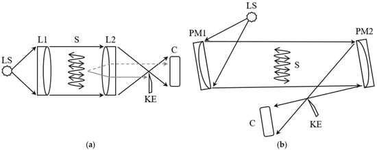
Figure 1. Diagrams of two types of schlieren instruments: (a) Toepler’s lens-type schlieren system; (b) z-type schlieren system using twin parabolic mirrors.

Therefore, in this study, the most commonly used Z-type Schlieren system was employed to visualize the behavior of CO₂ gas inside the tube.

2.2. Experimental Setup

Figure 2 shows a schematic diagram of the experimental setup used in this study, while Table 1 presents the specifications of the experimental apparatus. Air was compressed through a compressor and then controlled by a mass flow controller (MFC). Carbon dioxide gas was also controlled by the mass flow controller (MFC). Subsequently, the compressed air and carbon dioxide were mixed using a static mixer. The air mixed through the static mixer was introduced into the tube through nozzles that were formed tangentially inside the tube. The tube used in the experiment was designed differently from a conventional counter-flow vortex tube. In a typical counter-flow vortex tube, the fluid enters the tube tangentially along the nozzle of the vortex generator, forming vortices. However, in a typical counter-flow vortex tube, there are many components that can cause refraction along the optical path. Therefore, in this study, all components of the vortex tube that could cause refraction along the optical path were removed, and a tube with a single nozzle was designed and manufactured. To measure the temperature and pressure at the nozzle inlet, a thermocouple and a pressure sensor were placed between the static mixer and the nozzle. The Z-type Schlieren system was used to visualize the flow of the mixture inside the tube. The configuration of the Schlieren system included a 120 W LED light source, a parabolic mirror with a diameter of 150 mm and an f/8 focal ratio, and a knife-edge arranged horizontally. Schlieren images were captured using a Canon EOS 80D, along with a Canon lens with an aperture value of f/1.4. The video was recorded at a shutter speed of 1/4000, ISO 100, and 25 frames per second (fps).

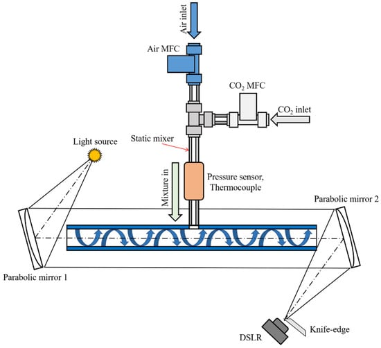
Figure 2. Schematic diagram of experimental equipment.

Table 1. Specification of experimental equipment.

Equipment	Specification
LED light source	Power	120 W
	Pinhole diameter	1 mm
Parabolic mirror	Diameter	150 mm
	Aperture	f/8
Tube	Length	560 mm
	Inner diameter	40 mm
	Nozzle diameter	1.5 mm
Thermocouple	Type	K-type
	Limits of error	1.1 °C or 0.4%
	Temperature range	−200 to 1250 °C
Pressure sensor	Range	0 to 10 bar
	Accuracy	±0.5% FS(RSS)

2.3. Experimental Method

The goal of this study was to visualize and analyze the behavior of the fluid in a mixed gas at a constant flow rate according to the CO₂ volume fraction. Therefore, to observe the effects of changes in CO₂ concentration on the flow and behavior of the fluid, the behavior of single-phase CO₂ flow and the air–CO₂ mixture fluid was analyzed. The supply flow rate of CO₂ and the air–CO₂ mixture was fixed at 9.0 L per minute (lpm). For the air–CO₂ mixture, the initial CO₂ volume fraction was incrementally changed from 0.2 to 0.8 in steps of 0.2 for the experiments as presented in Table 2. The initial temperature was set at approximately 24 °C during the experiments.

Table 2. Experimental conditions.

Total Flow Rate [lpm]	CO2 Volume Fraction [-]	Air Flow Rate [lpm]	CO2 Flow Rate [lpm]	Inlet Pressure [bar]	Inlet Temperature [°C]
9.0	0.2	7.2	1.8	0.97	24.31
	0.4	5.4	3.6	1.17	24.29
	0.6	3.6	5.4	1.32	24.27
	0.8	1.8	7.2	1.49	24.27

The experiment was conducted by opening the air MFC valve to match the target flow rate, and then opening the CO₂ MFC valve to allow the gases to flow into the tube in a mixed state through the static mixer. The cross-section of the tube was captured as shown in Figure 3, with a shutter speed of 1/25 s. A total recording time of 1.2 s (30 frames) was taken from the moment the mixture gas entered the tube. The captured images have a size of 1200 × 1200 pixels, and they were subsequently converted to grayscale images to compare pixel intensity. Each experimental condition was repeated multiple times to confirm qualitative repeatability of the observed flow behavior, and representative Schlieren images are presented in Section 3.

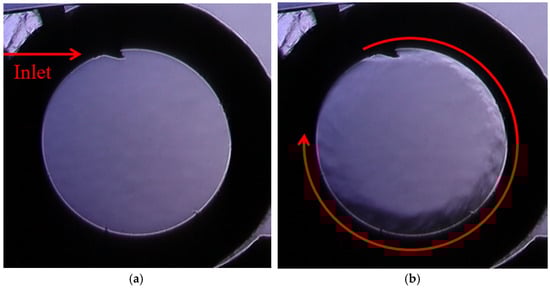
Figure 3. Example of flow visualization using the Schlieren method: (a) stable initial state; (b) the difference in brightness caused by the refraction of light.

2.4. Image Filter

Before analyzing the captured Schlieren images, it is necessary to apply a filter to remove noise from the images. Therefore, in this study, a two-dimensional Gaussian filter, which is a low-pass filter based on the Gaussian distribution, was applied. The Gaussian filter uses an interpolation method that incorporates the pixel intensity of each pixel along with the surrounding pixel intensities. It is defined using a Gaussian function with a given standard deviation, as follows [23]:

$$G\left(x, y\right)= {\displaystyle \frac{1}{2\pi {\sigma }^2}}{e}^{{\displaystyle \frac{-(x^2+y^2)}{2{\sigma }^2}}}$$

(1)

where x, y represent the relative positions from the center of the filter, and σ is the standard deviation.

3. Results and Discussion

3.1. Considerations on CO₂ Single-Phase Flow

Before analyzing the behavior of the air–CO₂ mixture inside the tube, the intention was to analyze the behavior of CO₂ gas within the tube. The captured Schlieren images underwent noise removal using a Gaussian filter, followed by background correction to eliminate brightness differences caused by density variations. This procedure enabled clearer visualization of the CO₂ flow field.

To evaluate the internal CO₂ distribution, the pixel intensity values were extracted within a circular mask corresponding to the inner flow field. Through calibration, it was confirmed that each pixel corresponded to approximately 0.037 mm. The total number of pixels analyzed inside the tube was 916,021.

Figure 4 shows the original Schlieren images of the CO₂ single-phase flow at different capture times (0.08–0.44 s). The overall contrast increased as time progressed and the boundary layers became more pronounced.

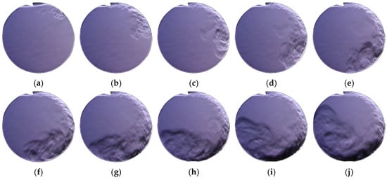
Figure 4. Original Schlieren images of CO₂ single-phase flow according to capture time: (a) 0.08 s, (b) 0.12 s, (c) 0.16 s, (d) 0.20 s, (e) 0.24 s, (f) 0.28 s, (g) 0.32 s, (h) 0.36 s, (i) 0.40 s, and (j) 0.44 s.

Figure 5 shows the corresponding background-corrected images obtained after subtracting the reference background taken under quiescent air. The brightness differences caused by refractive index variations were enhanced, allowing the CO₂ flow structures to appear more distinctly.

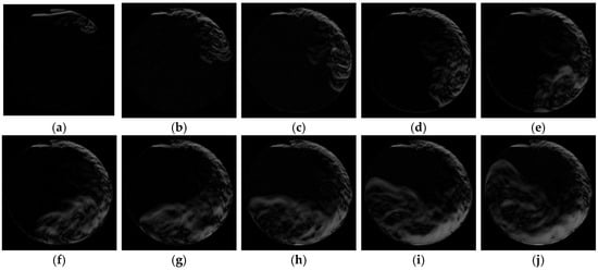
Figure 5. Background correction images of CO₂ single-phase flow according to capture time: (a) 0.08 s, (b) 0.12 s, (c) 0.16 s, (d) 0.20 s, (e) 0.24 s, (f) 0.28 s, (g) 0.32 s, (h) 0.36 s, (i) 0.40 s, and (j) 0.44 s.

Figure 6 shows the result of applying a circular mask to exclude the tube-wall region, thereby isolating only the internal flow field used for subsequent pixel intensity analysis.

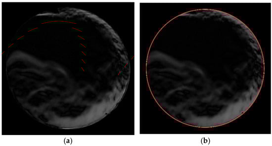
Figure 6. Example of post-processing a circular mask: (a) background correction image; (b) mask post-processing image.

Figure 7 shows the temporal variations of the mean and standard deviation of pixel intensity for each capture frame. The average pixel intensity increased with capture time, indicating the progressive development of high-intensity zones inside the tube. The minimum and maximum mean pixel intensity values were 2.85 and 30.47, respectively, while the standard deviation ranged from 12.92 to 29.29. The initial increase in the standard deviation reflects the growth of spatial non-uniformity in the Schlieren intensity field as vortex-induced structures and shear layers develop within the flow. After approximately 0.28 s, the gradual stabilization of the standard deviation suggests that the large-scale vortex structure becomes more established, leading to a relatively steady spatial distribution of the Schlieren signal despite ongoing flow evolution.

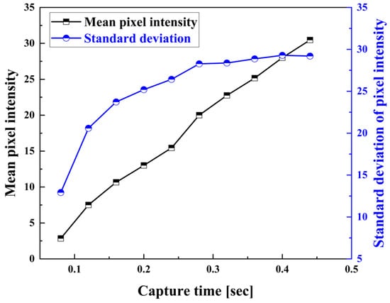
Figure 7. Mean pixel intensity and standard deviation in CO₂ single-phase flow.

To estimate the relative CO₂ indicator, the pixel intensity values were normalized between 0 and 255. It should be noted that the Schlieren technique visualizes refractive index gradients integrated along the optical path. Therefore, the recorded pixel intensity does not represent an absolute CO₂ concentration but rather indicates relative variation in density or refractive index within the flow field. This normalization provides a qualitative indicator of regions associated with relatively high CO₂ presence and enables comparative discussion among successive frames rather than producing a quantitative concentration map.

Figure 8 shows the temporal evolution of the normalized CO₂ distribution ratio. Figure 8a, the fraction of pixels within the 0–5% intensity range continuously decreases, whereas Figure 8b, which excludes that range, shows an increase in the proportion of higher intensity regions. This complementary behavior indicates an apparent redistribution of high-intensity regions associated with CO₂ toward the vortex region during the single-phase flow.

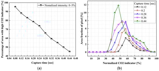
Figure 8. Relative CO₂ indicator distribution in CO₂ single-phase flow: (a) distribution including the lowest normalized intensity range; (b) distribution excluding the lowest normalized intensity range.

Because the Schlieren image corresponds to a two-dimensional projection of a three-dimensional turbulent flow, the measured intensity inherently includes line-of-sight averaging effects. Local fluctuations along the optical axis are integrated, and fine three-dimensional structures may be partially obscured. Despite this limitation, the relative contrast distribution still provides meaningful qualitative insight into the spatial behavior and transport of CO₂ within the tube.

Figure 9 shows the contour of regions with normalized intensity values exceeding 80% within the tube cross-section. These high-intensity zones correspond to regions of relatively high Schlieren intensity formed immediately after discharge from the nozzle. The flow field shows that the injected flow follows the inner wall, forming a vortex structure and returning toward the nozzle region after approximately 0.44 s, completing one rotation. Due to the line-of-sight integration inherent to the Schlieren technique, absolute concentration values cannot be determined. Nevertheless, this visualization qualitatively indicates that relatively high-intensity regions tend to appear near the right-hand side of the tube relative to its vertical axis, where centrifugal effects are expected to be stronger.

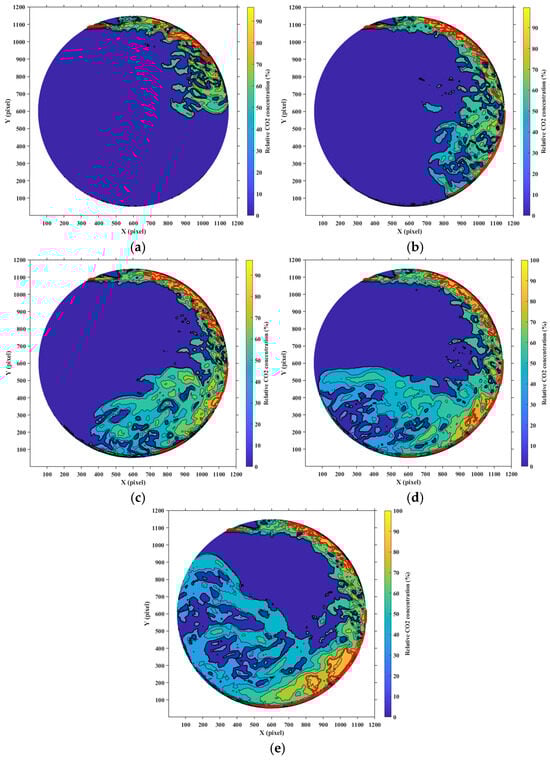
Figure 9. CO₂ concentration contour in tube cross-section (values above 80% indicated a red line): (a) 0.12 s, (b) 0.20 s, (c) 0.28 s, (d) 0.36 s, and (e) 0.44 s.

3.2. Considerations in Air–CO₂ Mixture Flow

After investigating the single-phase CO₂ flow, the air–CO₂ mixture was examined under the same optical configuration. All Schlieren images were processed with Gaussian filtering and background correction identical to those described above. Given the qualitative nature of the Schlieren visualization, the pixel intensity analysis in the section was also treated as a relative comparison among different inlet CO₂ volume fractions rather than a quantitative measurement. The contrast variations, therefore, reflect the spatial distribution tendency of CO₂-related Schlieren intensity within the mixture, influenced by tangential injection and vortex motion.

Figure 10, Figure 11, Figure 12 and Figure 13 show the original and filtered images taken between 0.08 and 0.20 s, based on varying inlet CO₂ volume fractions. As the inlet CO₂ volume fraction increases, it can be observed that the contrast in the images becomes more pronounced, and the boundary layer shapes also become clearer. However, with a capture time of 0.08 s for inlet CO₂ volume fractions of 0.2 and 0.4, it is difficult to clearly observe the behavior of the CO₂ fluid and the boundary layer shapes due to the low CO₂ concentration. Therefore, a relative intensity-based analysis using pixel intensity was conducted, similar to the analysis of the behavior of the CO₂ fluid.

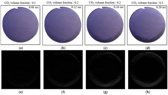
Figure 10. Original image and background correction image at inlet CO₂ volume fraction 0.2: (a) original image at 0.08 s; (b) original image at 0.12 s; (c) original image at 0.16 s; (d) original image at 0.20 s; (e) background correction image at 0.08 s; (f) background correction image at 0.12 s; (g) background correction image at 0.16 s; (h) background correction image at 0.20 s.

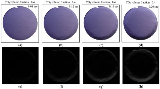
Figure 11. Original image and background correction image at inlet CO₂ volume fraction 0.4: (a) original image at 0.08 s; (b) original image at 0.12 s; (c) original image at 0.16 s; (d) original image at 0.20 s; (e) background correction image at 0.08 s; (f) background correction image at 0.12 s; (g) background correction image at 0.16 s; (h) background correction image at 0.20 s.

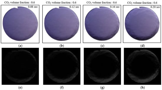
Figure 12. Original image and background correction image at inlet CO₂ volume fraction 0.6: (a) original image at 0.08 s; (b) original image at 0.12 s; (c) original image at 0.16 s; (d) original image at 0.20 s; (e) background correction image at 0.08 s; (f) background correction image at 0.12 s; (g) background correction image at 0.16 s; (h) background correction image at 0.20 s.

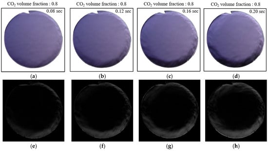
Figure 13. Original image and background correction image at inlet CO₂ volume fraction 0.8: (a) original image at 0.08 s; (b) original image at 0.12 s; (c) original image at 0.16 s; (d) original image at 0.20 s; (e) background correction image at 0.08 s; (f) background correction image at 0.12 s; (g) background correction image at 0.16 s; (h) background correction image at 0.20 s.

Figure 14 shows the average pixel intensity and the standard deviation of pixel intensity based on the inlet CO₂ volume fraction. As the capture time increases, there is a tendency for both the average pixel intensity and the standard deviation of the Schlieren intensity field inside the tube to increase. The average pixel intensity and the standard deviation of pixel intensity showed relatively higher values as the inlet CO₂ volume fraction increased. The mean pixel intensity characterizes the overall Schlieren signal level averaged over the region of interest, whereas the standard deviation is associated with the spatial distribution of the intensity field. Because these two metrics capture different features of the Schlieren signal, their temporal evolution may differ, which can lead to overlaps appearing at different capture times.

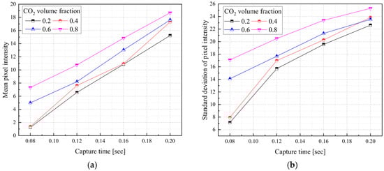
Figure 14. Mean pixel intensity and standard deviation according to inlet CO₂ volume fraction: (a) mean pixel intensity; (b) standard deviation of pixel intensity.

Figure 15 shows the proportion of pixels with normalized intensity exceeding 10% within the flow field area inside the tube, based on capture time for the air–CO₂ mixture. For all inlet CO₂ volume fraction conditions, the area corresponding to the lowest normalized intensity range (0–5%) inside the tube decreased over time, while the proportion of pixels with normalized intensity exceeding 30% exhibited an increasing trend.

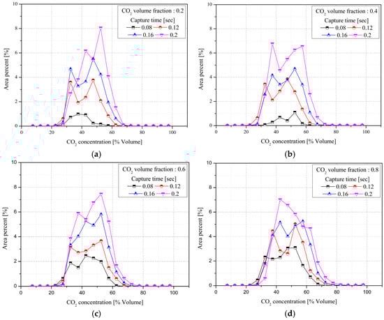
Figure 15. Relative CO₂ indicator distribution of 5–100% according to inlet volume fraction: (a) CO₂ volume fraction 0.2; (b) CO₂ volume fraction 0.4; (c) CO₂ volume fraction 0.6; (d) CO₂ volume fraction 0.8.

Figure 16 shows the result of masking pixels with normalized intensity exceeding 60% in the contour of the air–CO₂ mixture at a capture time of 0.20 s. Unlike the previous single-phase CO₂ flow, regions with normalized intensity exceeding 80% did not appear in the tube cross-section. In addition, it was observed that the time required for the injected flow to travel from the nozzle and complete one rotational path along the tube wall was shorter than that observed in the single-phase flow.

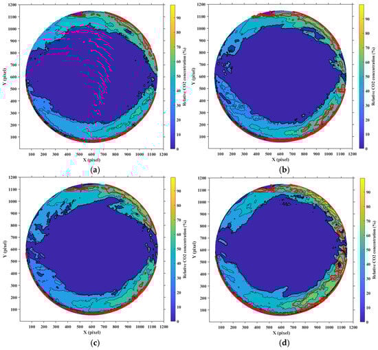
Figure 16. CO₂-related Schlieren intensity contour of the tube cross-section at a capture time of 0.20 s (values above 60% indicated a red line): (a) CO₂ volume fraction 0.2; (b) CO₂ volume fraction 0.4; (c) CO₂ volume fraction 0.6; (d) CO₂ volume fraction 0.8.

In the air–CO₂ mixture experiment, air was introduced into the tube through the MFC while the CO₂ MFC valve was opened for mixing, resulting in a reduced residence time of the injected flow compared to the single-phase CO₂ case. The inlet CO₂ volume fraction of 0.8 showed the broadest distribution of regions with normalized intensity exceeding 60%. The relative intensity distribution of the air–CO₂ mixture exhibited a trend similar to that observed for the single-phase CO₂ flow. The distribution of regions with normalized intensity exceeding 60% was predominantly located on the right-hand side toward the nozzle exit, relative to the central axis of the tube.

4. Conclusions

In this study, the behavior of CO₂ gas in the vortex flow of both CO₂ single-phase and air–CO₂ mixture flows inside a vortex tube was visualized using the Schlieren method, and a relative distribution analysis was conducted. The results demonstrate that the temporal evolution of the normalized Schlieren pixel intensity and its standard deviation provides useful quantitative indicators for characterizing the development of vortex flow structures in a relative sense. In particular, consistent trends were observed in the growth and subsequent stabilization of spatial non-uniformity within the tube, reflecting the progressive development of vortex-induced structures under the tested operating conditions. Based on these observations, the following conclusions are drawn:

• Characteristics of Single-Phase CO₂ Flow

The filtered Schlieren images allowed for clear observation of the boundary layer shapes generated by the density differences of CO₂ gas, showing a tendency for the relative Schlieren intensity associated with CO₂-rich regions to increase over time. Areas with normalized intensity exceeding 80% were primarily concentrated near the core region at the nozzle exit and on the right side of the tube, relative to the center towards the nozzle exit.

2.

Flow Analysis of Air–CO₂ Mixture

As the inlet CO₂ volume fraction increased, the contrast of Schlieren images became more pronounced, and the boundary layer shapes became clearer. Similar to single-phase flow, relatively high-intensity regions appeared near the nozzle exit, following the vortex trajectory.

3.

Limitations and Future Work

Because the Schlieren technique represents an optical integration along the line of sight, the present analysis provides qualitative indicators rather than absolute CO₂ concentration fields. The results should thus be interpreted as relative distributions indicating comparative density variation under different operating conditions. Future research will incorporate calibration procedures using interferometric or absorption-based diagnostics to quantitatively correlate Schlieren intensity with local refractive index or CO₂ concentration fields.

4.

Potential of Gas Separation Technology

Despite these limitations, the visualization revealed that regions of relatively high Schlieren intensity consistently appeared in specific locations within the tube, suggesting that the observed relative distribution is sensitive to local flow features near the nozzle region under the present experimental configuration. This study, therefore, provides foundational qualitative insight into vortex-induced flow behavior that may be relevant to future studies on gas separation mechanisms.

Future work may extend the present investigation to a wider range of operating conditions, including higher inlet velocities and alternative nozzle configurations. In addition, coupling Schlieren-based visualization with numerical simulations could provide complementary insight into the internal flow behavior of vortex tubes.

References

- Keith, D.W.; Holmes, G.; Angelo, D.S.; Heidel, K. A Process for Capturing CO2 from the Atmosphere. Joule 2018, 2, 1573–1594. [Google Scholar] [CrossRef]
- Younas, M.; Sohail, M.; Kong, L.L.; Bashir, M.J.K.; Sethupathi, S. Feasibility of CO2 Adsorption by Solid Adsorbents: A Review on Low-Temperature Systems. Int. J. Environ. Sci. Technol. 2016, 13, 1839–1860. [Google Scholar] [CrossRef]
- Osman, A.I.; Hefny, M.; Abdel Maksoud, M.I.A.; Elgarahy, A.M.; Rooney, D.W. Recent Advances in Carbon Capture Storage and Utilisation Technologies: A Review. Environ. Chem. Lett. 2020, 19, 797–849. [Google Scholar] [CrossRef]
- Yun, J.; Kim, Y.; Yu, S. Feasibility Study of Carbon Dioxide Separation from Gas Mixture by Vortex Tube. Int. J. Heat Mass Transf. 2018, 126, 353–361. [Google Scholar] [CrossRef]
- Subudhi, S.; Sen, M. Review of Ranque-Hilsch Vortex Tube Experiments Using Air. Renew. Sustain. Energy Rev. 2015, 52, 172–178. [Google Scholar] [CrossRef]
- Saidi, M.H.; Valipour, M.S. Experimental Modeling of Vortex Tube Refrigerator. Appl. Therm. Eng. 2003, 23, 1971–1980. [Google Scholar] [CrossRef]
- Thakare, H.R.; Parekh, A.D. Experimental Investigation of Ranque-Hilsch Vortex Tube and Techno-Economical Evaluation of Its Industrial Utility. Appl. Therm. Eng. 2020, 169, 114934. [Google Scholar] [CrossRef]
- Agarwal, G.; McConkey, Z.P.; Hassard, J. Optimisation of Vortex Tubes and the Potential for Use in Atmospheric Separation. J. Phys. D Appl. Phys. 2020, 54, 015502. [Google Scholar] [CrossRef]
- Bazgir, A. Analyzing Separation Capacity Efficiency of a Binary Hydrocarbon System (Cyclohexane-N-Pentane) with the Help of Two Distinct Methods: Utilizing A Vortex Tube Separator and An Equilibrium Flash Stage (EFS). Exp. Therm. Fluid Sci. 2019, 109, 109853. [Google Scholar] [CrossRef]
- Mohammadi, S.; Farhadi, F. Experimental and Numerical Study of the Gas–Gas Separation Efficiency in a Ranque-Hilsch Vortex Tube. Sep. Purif. Technol. 2014, 138, 177–185. [Google Scholar] [CrossRef]
- Linderstrøm-Lang, C.U. Gas Separation in the Ranque-Hilsch Vortex Tube. Int. J. Heat Mass Transf. 1964, 7, 1195–1206. [Google Scholar] [CrossRef]
- Kulkarni, M.R.; Sardesai, C.R. Enrichment of Methane Concentration via Separation of Gases Using Vortex Tubes. J. Energy Eng. 2002, 128, 1–12. [Google Scholar] [CrossRef]
- Van Trinh, N.; Kim, Y.; Im, S.; Kim, B.J.; Park, S.H.; Yu, S. Parametric Investigation of CO2 Separation Performance from Air-CO2 Mixture at the Cold Outlet of the Vortex Tube. Int. J. Heat Mass Transf. 2024, 233, 126040. [Google Scholar] [CrossRef]
- Van Trinh, N.; Kim, Y.; Pae, W.; Im, S.; Kim, B.; Yu, S. Effect of cyclone on the CO2 separation characteristics of vortex tube. Sep. Purif. Technol. 2025, 359, 130580. [Google Scholar] [CrossRef]
- Dutta, T.; Sinhamahapatra, K.P.; Bandyopadhyay, S.S. Numerical investigation of gas species and energy separation in the Ranque-Hilsch vortex tube using real gas model. Int. J. Refrig. 2011, 34, 2118–2128. [Google Scholar] [CrossRef]
- Gholami, V.; Jafarian, S.M.M. Optimization of large-scale Ranque-Hilsch vortex tube for enhanced CO2 separation in carbon capture and storage. Gas Sci. Eng. 2024, 145, 205788. [Google Scholar] [CrossRef]
- Settles, G.S.; Hargather, M.J. A Review of Recent Developments in Schlieren and Shadowgraph Techniques. Meas. Sci. Technol. 2017, 28, 042001. [Google Scholar] [CrossRef]
- Merzkirch, W. Flow Visualization; Academic: New York, NY, USA, 1987; ISBN 0-12-491351-2. [Google Scholar]
- Kook, S.; Le, M.K.; Padala, S.; Hawkes, E.R. Z-Type Schlieren Setup and Its Application to High-Speed Imaging of Gasoline Sprays. SAE Tech. Pap. 2011, 1, 1981. [Google Scholar] [CrossRef]
- Traldi, E.; Boselli, M.; Simoncelli, E.; Stancampiano, A.; Gherardi, M.; Colombo, V.; Settles, G.S. Schlieren Imaging: A Powerful Tool for Atmospheric Plasma Diagnostic. EPJ Tech. Instrum. 2018, 5, 4. [Google Scholar] [CrossRef]
- Settles, G.S. Schlieren and Shadowgraph Techniques: Visualizing Phenomena in Transparent Media; Springer Science & Business Media: Berlin/Heidelberg, Germany, 2001. [Google Scholar]
- Machado, D.A.; de Souza Costa, F.; de Andrade, J.C.; Dias, G.S.; Fischer, G.A.A. Schlieren Image Velocimetry of Swirl Sprays. Flow. Turbul. Combust. 2023, 110, 489–513. [Google Scholar] [CrossRef]
- Deng, G.; Cahill, L.W. Adaptive Gaussian Filter for Noise Reduction and Edge Detection. IEEE Nucl. Sci. Symp. Med. Imaging Conf. 1994, 3, 1615–1619. [Google Scholar] [CrossRef]
Disclaimer/Publisher’s Note: The statements, opinions and data contained in all publications are solely those of the individual author(s) and contributor(s) and not of MDPI and/or the editor(s). MDPI and/or the editor(s) disclaim responsibility for any injury to people or property resulting from any ideas, methods, instructions or products referred to in the content. |
© 2025 by the authors. Licensee MDPI, Basel, Switzerland. This article is an open access article distributed under the terms and conditions of the Creative Commons Attribution (CC BY) license.