A Phenomenological Boundary Layer Approach to Interpret the Structure of the Heat Transfer Correlations for Laminar Forced Convection over Isothermal Flat Plates

Abstract

Forced convection heat transfer is commonly described by a correlation of the type $Nu=AR{e}^{\gamma }P{r}^{\lambda }$, where $\lambda <\gamma$ for moderate-to-high-Pr fluids, whereas $\lambda =\gamma$ for low-Pr fluids. Yet, the phenomenological basis of this structure is seldom examined. This work shows that such a correlation can be interpreted from purely physical intuition, without employing scaling arguments or solving the governing equations. Focusing on laminar flow over an isothermal flat plate, we introduce a new phenomenological boundary layer approach in which, by assessing how each independent variable qualitatively affects the thickness of the boundary layer, we construct the proportionality of $Nu$ on $Re$ and $Pr$. The approach provides a physical interpretation of why the exponents of established forced convection correlations fall within certain ranges. This perspective may help both educators seeking intuition-based explanations and researchers exploring alternative formulations of forced convection heat transfer.

1. Introduction

Forced convection heat transfer plays an important role in several engineering applications. Moderate-to-high-$Pr$ fluids are typically used in electronic cooling, process heat exchangers, drying technologies and automobile industry applications, to name a few, as reported by Murshed et al. [1], Marzouk et al. [2], Santos et al. [3] and Barmavatu et al. [4], respectively. On the other hand, low-$Pr$ fluids are employed for cooling purposes in nuclear and concentrated solar power plants, as reported by Agbevanu et al. [5] and Lorenzin et al. [6], as well as in many other applications (see, e.g., Deng et al. [7] and Heinzel et al. [8]). However, their use is still limited, mainly due to their corrosivity, which raises significant pumping concerns, as outlined by Qin et al. [9].

To discuss the main features of forced convection heat transfer, reference is usually made to the classical configuration of steady incompressible laminar flow adjacent to an isothermal flat plate having a temperature $T_p$ higher than the temperature $T_{\infty }$ of the undisturbed fluid, as it represents the simplest configuration in which the fundamental coupling between momentum and energy transport can be clearly examined.

Indeed, the flat plate configuration is typically used in almost all textbooks to illustrate the fundamental physical principles underlying external forced convection flows (see, e.g., Gebhart [10], Incropera et al. [11] and Kreith et al. [12]).

The pioneering works on this topic were conducted by Blasius [13] and Pohlhausen [14], who solved the boundary layer differential equations to determine the velocity and the temperature fields, respectively, as well as the corresponding thicknesses, $\delta$ and ${\delta }_t$, of the velocity and thermal boundary layers, whose characteristics have been extensively discussed in Schlichting et al. [15]. Specifically, Blasius introduced a similarity variable which can be interpreted as the ratio between the distance z normal to the plate and the thickness $\delta$ of the velocity boundary layer at a given distance x from the leading edge of the plate, where $\delta$ can be estimated from a scale analysis of the balance between inertial and viscous forces, yielding the dimensionless relationship

$${\displaystyle \frac{\delta }{x}}\sim {\displaystyle \frac{1}{R{e}^{1/2}}}$$

(1)

This result highlights that the Reynolds number, whose physical meaning and role have been extensively discussed in the recent papers by Saldana et al. [16] and Tamburrino et al. [17], is the key dimensionless group governing the thickness of the velocity boundary layer.

Once the similarity variable is introduced into the continuity and momentum equations, a similarity velocity profile in the direction normal to the plate at any position x along the plate is obtained numerically, together with the value of the coefficient relating the left- and right-hand sides of Equation (1).

Subsequently, Pohlhausen substituted a polynomial approximation of the velocity field obtained by Blasius into the energy equation, which he then solved for moderate-to-high-$Pr$ fluids, thereby deriving the following heat transfer correlation

$$Nu=0.332R{e}^{1/2}P{r}^{1/3}(Pr\ge 0.6)$$

(2)

Later, different authors solved the energy equation for low-$Pr$ fluids. In particular, Sparrow and Gregg [18] obtained exact solutions for some values of the Prandtl number, leading to the correlation

$$Nu=A\left(Pr\right)R{e}^{1/2}P{r}^{1/2}(Pr\le 0.03)$$

(3)

where the coefficient $A\left(Pr\right)$ exhibits a weak dependence on the Prandtl number, as shown in Figure 1, together with an approximate function previously proposed by Morgan [19], who also determined the asymptotic value $A=0.564$ for $Pr\to 0$.

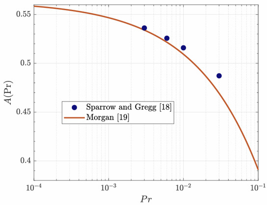
Figure 1. Plotof the coefficient $A\left(Pr\right)$ versus the Prandtl number.

More recently, Bejan [20] applied scaling arguments to the energy equation and recovered the same proportionalities of Equations (2) and (3), assuming that the velocity profile within the thermal boundary layer is linear for high-$Pr$ fluids and uniform for low-$Pr$ fluids. An interesting outcome of scale analysis is that it simplifies the governing differential equations by replacing each term with its order of magnitude. This transforms the differential equations into algebraic relations between dominant terms—such as inertia versus friction in the momentum equation, and convection versus conduction in the energy equation. As a result, after simple algebra, relationships like those reported in Equations (1)–(3) naturally emerge as power law dependencies.

For the sake of completeness, it is worth noting that, in order to generalize the results found for both moderate-to-high-$Pr$ fluids and low-$Pr$ fluids, Churchill and Ozoe [21] formulated a unique correlation valid for the entire range of the Prandtl number. Additionally, correlations including both laminar and turbulent flow regimes, such as those proposed by Gnielinksi [22], Ahmed et al. [23], Lienhard et al. [24] and Zhao et al. [25], were also developed.

In this framework, the aim of the present paper is to interpret the structure of the correlations expressed by Equations (2) and (3) through a new phenomenological boundary layer approach, without invoking either the similarity solutions or the scaling of the governing differential equations. In particular, such an approach seeks to determine—based solely on physical reasoning—whether each independent variable leads to an increase or a decrease in the thickness of the thermal boundary layer, which, acting as a thermal resistance to heat transfer, is inversely proportional to the convection heat transfer coefficient. Once the influence of each variable has been identified, the resulting individual proportionality relationships are properly combined to obtain the direct proportionality between the Nusselt number and the Reynolds and Prandtl numbers. Of course, as our approach does not rely on quantitative equations, it cannot specify a precise functional dependence between the Nusselt number and the Reynolds and Prandtl numbers. On the other hand, once the power law dependence is adopted, our approach cannot provide specific values of the exponents, but only physically consistent ranges. Despite this, our step-by-step approach, which does not require any advanced mathematical knowledge, provides a novel pedagogical method, as well as a new interpretation of the structure of the heat transfer correlations, useful for both educators and researchers.

2. The Phenomenology Behind the Blasius Solution

In forced convection, the fluid motion is not affected by heat transfer, at least as far as the physical properties of the fluid can be assumed constant. This allows the characteristics of the velocity boundary layer to be determined independently of the existence of a temperature field. On the other hand, the study of the velocity boundary layer is essential to derive the main characteristics of the temperature field, which is the primary focus of the present study.

In the examined configuration, the flow is driven by an imposed undisturbed fluid velocity $u_{\infty }$ parallel to the plate, remaining substantially parallel to the plate. As a result, the velocity x-component along the plate is by far dominant compared to the velocity z-component normal to the plate, which, although essential to satisfy flow continuity within the boundary layer, is sufficiently small to be neglected for an analysis of the physics underlying the overall flow motion parallel to the plate.

Due to viscous friction exerted by the plate, a fluid element moving in laminar flow parallel to the plate at a given normal distance z gradually slows down with increasing distance x from the leading edge. Hence, the velocity profile, which starts from $u=0$ at $z=0$ and asymptotically approaches $u=u_{\infty }$ at $z=\delta$, undergoes a sort of stretching in the direction normal to the plate as x increases. Accordingly, the thickness $\delta$ of the velocity boundary layer increases with x starting from a conventional zero value at the leading edge of the plate, as shown in Figure 2. Moreover, the increase of $\delta$ with x must occur with a decreasing gradient $d\delta /dx$. This is because, in the near-wall region where viscous effects are significant, as the fluid moves along x, the local decrease in velocity leads to a reduction of the velocity gradient normal to the plate, resulting in a decrease in the shear stress. Consequently, the fluid decelerates progressively less, and the stretching of the velocity profile in the direction normal to the plate becomes progressively less pronounced.

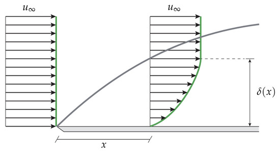
Figure 2. The velocity profile and the velocity boundary layer over a flat plate.

Additionally, the thickness of the velocity boundary layer is also directly proportional to the fluid’s kinematic viscosity $\nu =\mu /\rho$. In fact, a higher value of $\nu$ corresponds to a higher aptitude of the fluid to propagate the friction exerted by the plate through the velocity boundary layer. This arises as a direct consequence of the competition between the effects of the fluid’s dynamic viscosity $\mu$, which is a measure of the shear stress produced inside the fluid, and the fluid’s mass density $\rho$, which is a measure of the mechanical inertia of the fluid.

Finally, also the undisturbed fluid velocity $u_{\infty }$ plays an important role in determining the thickness of the velocity boundary layer. Actually, an increase of $u_{\infty }$ directly leads to an increase of the fluid momentum, thereby increasing the fluid’s inertia, which would tend to decrease the thickness of the velocity boundary layer. On the other hand, an increase of $u_{\infty }$ leads to a growth of the component of the velocity gradient in the direction normal to the plate, which, enhancing the local shear stress, would tend to reduce the fluid velocity with a consequent increase of the thickness of the velocity boundary layer. Overall, the first effect is dominant, thus implying that an increase in $u_{\infty }$ results in a decrease of the thickness of the velocity boundary layer.

Ultimately, the thickness $\delta$ of the velocity boundary layer depends on the distance x from the leading edge of the plate, the fluid’s kinematic viscosity $\nu$, and the undisturbed fluid velocity $u_{\infty }$, as follows:

$$\delta \propto x\left(withdecreasing{\displaystyle \frac{\partial \delta }{\partial x}}\right),\delta \propto \nu ,\delta \propto {\displaystyle \frac{1}{u_{\infty }}}$$

(4)

where the proportionality symbol “∝” should be interpreted simply as “increases with”, without implying any specific functional dependence between the related quantities. Conversely, whenever in the paper a precise functional dependence is specified, the proportionality symbol “∼” is adopted—as, e.g., done in Equation (1), where the functional dependence is a power law. Given these definitions, it is clear that the proportionality symbol “∼” conveys more specific information than the proportionality symbol “∝”.

With the aim to express the thickness of the velocity boundary layer in dimensionless form, i.e., as $\delta /x$, the right-hand side of the corresponding relation must be dimensionless as well. This means that $\delta /x$ must depend on x, $\nu$ and $u_{\infty }$ through an appropriate combination of these independent variables assembled into one or more dimensionless groups in which any of such variables must necessarily be included using a power law expression. So, given that x has dimensions of [m], $\nu$ has dimensions of [m²/s], and $u_{\infty }$ has dimensions of [m/s], the simplest and most straightforward way to combine these variables into a single dimensionless group accounting as far as possible for the direct and inverse proportionalities expressed by Equation (4) is

$${\displaystyle \frac{\delta }{x}}\propto {\displaystyle \frac{\nu }{x{u}_{\infty }}}$$

(5)

Naturally, while the second and third proportionality relationships reported in Equation (4) are automatically satisfied, an appropriate functional dependence between the left- and right-hand sides of Equation (5) must be introduced to also satisfy the first proportionality relationship.

Notice that the inverse of the right-hand side of Equation (5) is the Reynolds number:

$$Re={\displaystyle \frac{x{u}_{\infty }}{\nu }}$$

(6)

Therefore, Equation (5) becomes

$${\displaystyle \frac{\delta }{x}}\propto {\displaystyle \frac{1}{Re}}$$

(7)

Actually, this result can be easily justified by the fact that the dimensionless thickness of the velocity boundary layer is directly related to the competition existing between the viscous and inertial forces, whose intensity is exactly quantified by the inverse of the Reynolds number.

Of course, a precise functional dependence must be introduced in order to allow for the required direct proportionality between $\delta$ and x, enforcing also that the velocity boundary layer should increase with a decreasing gradient. Yet, the present approach is not able to determine a specific functional structure. Indeed, according to the result obtained by Blasius expressed by Equation (1), such a dependence is a power law with an exponent $1/2$.

3. The Phenomenology Behind the Pohlhausen Correlation

A generic fluid element moving in laminar flow parallel to the plate at any given distance z from the plate gradually warms up as it enters the influence region of the plate by receiving heat by the adjacent fluid layer closer to the plate, which leads to the development of a thermal boundary layer, whose local thickness is denoted as ${\delta }_t$. Therefore, at each distance z from the plate, the fluid temperature increases with an increase in distance x from the leading edge of the plate. Hence, the temperature profile, which starts from $T=T_p$ at $z=0$ and asymptotically approaches $T=T_{\infty }$ at $z={\delta }_t$, undergoes a sort of stretching in the direction normal to the plate. Accordingly, the thickness ${\delta }_t$ of the thermal boundary layer increases with x starting from a conventional zero value at $x=0$, as shown in Figure 3. Indeed, the increase of ${\delta }_t$ with x must occur with a decreasing gradient $d{\delta }_t/dx$, since the fluid temperature rises progressively less along its path. This is because, in the near-wall region where heat transfer is significant, the local increase in temperature leads to a reduction of the temperature gradient normal to the plate. Consequently, the fluid temperature increases progressively less, and the stretching of the temperature profile in the direction normal to the plate becomes progressively less pronounced.

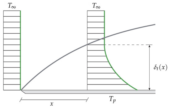
Figure 3. The temperature profile and the thermal boundary layer over a flat plate.

Moreover, the thickness of the thermal boundary layer is also directly proportional to the fluid’s thermal diffusivity $\alpha =k/c_p\rho$. In fact, a higher value of $\alpha$ corresponds to a higher aptitude of the fluid to rapidly modify its temperature in response to the heat received by the plate. This arises as a direct consequence of the competition between the effects of the fluid’s thermal conductivity k, which is a measure of the amount of heat transferred through the fluid, and the fluid’s heat capacity per unit volume $c_p\rho$, which is a measure of the thermal inertia of the fluid. Therefore, the temperature rise experienced by the fluid over the time interval required to reach a certain distance from the leading edge of the plate increases with $\alpha$, which implies that the temperature profile undergoes a more pronounced stretching in the direction normal to the plate, resulting in a thickening of the thermal boundary layer.

Finally, ${\delta }_t$ increases as the average velocity of the fluid within the thermal boundary layer decreases. This is because a lower average velocity implies a longer time for the fluid to reach a given distance from the leading edge of the plate, allowing more heat to be transferred from the plate to the fluid and producing a greater temperature rise. Consequently, the temperature profile stretches further in the direction normal to the plate, resulting in a thicker thermal boundary layer. On the other hand, the average fluid velocity within the thermal boundary layer decreases as the thickness of the velocity boundary layer increases, which is due to the reduction of the fluid velocity in the proximity of the plate, thus implying that the thickness of the thermal boundary layer increases as the thickness of the velocity boundary layer increases. Accordingly, on the basis of the earlier discussion on the thickness of the velocity boundary layer, ${\delta }_t$ is directly proportional to the fluid’s kinematic viscosity $\nu$ and inversely proportional to the undisturbed fluid velocity $u_{\infty }$.

Overall, the following proportionalities can be stated:

$${\delta }_t\propto x\left(withdecreasing{\displaystyle \frac{\partial {\delta }_t}{\partial x}}\right),{\delta }_t\propto \alpha ,{\delta }_t\propto \nu ,{\delta }_t\propto {\displaystyle \frac{1}{u_{\infty }}}$$

(8)

With the aim to express the thickness of the thermal boundary layer in dimensionless form, i.e., as ${\delta }_t/x$, the right-hand side of the corresponding relation must be dimensionless as well. This means that, following the same procedure used to derive the dimensionless thickness of the velocity boundary layer, ${\delta }_t/x$ must depend on x, $\alpha$, $\nu$ and $u_{\infty }$ through an appropriate combination of these independent variables assembled into one or more dimensionless groups in which any of such variables must necessarily be included using a power law expression, also accounting as far as possible for the direct and inverse proportionalities expressed by Equation (8).

Thus, the first, third and fourth relationships of Equation (8) can be grouped together in order to form the inverse of the Reynolds number, leading to

$${\displaystyle \frac{{\delta }_t}{x}}\propto {\displaystyle \frac{1}{Re}}$$

(9)

which, according to Equation (7), reflects the mentioned direct dependence between the thicknesses of the thermal and velocity boundary layers.

On the other hand, the dependence of ${\delta }_t$ on the thermal diffusivity $\alpha$ must also be taken into account. Since $\alpha$ and the $\nu$ share the same units [m²/s], the dimensionless thickness of the thermal boundary layer can be assumed to be proportional to the ratio between $\alpha$ and $\nu$, thus meaning

$${\displaystyle \frac{{\delta }_t}{x}}\propto {\displaystyle \frac{\alpha }{\nu }}$$

(10)

Notably, the inverse of the right-hand side of Equation (10) is the Prandtl number $Pr=\nu /\alpha$.

Therefore, on account of Equations (9) and (10), the following proportionalities hold:

$${\displaystyle \frac{{\delta }_t}{x}}\propto {\displaystyle \frac{1}{Re}},{\displaystyle \frac{{\delta }_t}{x}}\propto {\displaystyle \frac{1}{Pr}}$$

(11)

Now, with the aim to interpret the structure of the heat transfer correlation, based on the well-established power law dependence expressed by Equation (2), we can write

$${\displaystyle \frac{{\delta }_t}{x}}\sim {\displaystyle \frac{1}{R{e}^{\gamma }P{r}^{\lambda }}}$$

(12)

Notice that, once a power law dependence is adopted, the requirement of a direct proportionality between ${\delta }_t$ and x imposes that the exponent $\gamma$ of the Reynolds number must be lower than unity. Additionally, the further requirement of a direct proportionality between ${\delta }_t$ and $\nu$ imposes that the exponent $\lambda$ of the Prandtl number must be lower than the exponent $\gamma$ of the Reynolds number. This means that the following condition must hold: $0<\lambda <\gamma <1$.

Finally, since the heat flux exchanged between the plate and the fluid can be evaluated using the Fourier’s law applied to the fluid film adherent to the plate, we can write:

$$h_c\left(T_p-T_{\infty }\right)=-k{\left({\displaystyle \frac{\partial T}{\partial z}}\right)}_0$$

(13)

where ${\left(\partial T/\partial z\right)}_0$ is the component of the temperature gradient in the z-direction, normal to the plate, evaluated at the plate surface. Its order of magnitude can be estimated by assuming that the temperature profile within the thermal boundary layer is linear:

$${\left({\displaystyle \frac{\partial T}{\partial z}}\right)}_0\sim {\displaystyle \frac{T_{\infty }-T_p}{{\delta }_t}}$$

(14)

Substituting Equation (14) into Equation (13), we have

$$h_c\sim {\displaystyle \frac{k}{{\delta }_t}}$$

(15)

Subsequently, the combination of Equations (12) and (15) leads to the relationship

$${\displaystyle \frac{h_{c}x}{k}}\sim R{e}^{\gamma }P{r}^{\lambda }(0<\lambda <\gamma <1)$$

(16)

that, taking into account the definition of the Nusselt number, $Nu=h_{c}x/k$, can be written as

$$Nu\sim R{e}^{\gamma }P{r}^{\lambda }(0<\lambda <\gamma <1)$$

(17)

fully aligned with the Pohlhausen correlation reported in Equation (2), where the exponents $\gamma$ and $\lambda$ were found to be equal to $1/2$ and $1/3$, respectively. After all, the exponent $\gamma$ in Equation (17), directly derived from Equation (12), is expected to be $1/2$, as the thickness of the thermal boundary layer directly derives from the thickness of the velocity boundary layer, which, according to Equation (1), is inversely proportional to $R{e}^{1/2}$.

4. The Phenomenology Behind the Sparrow–Gregg Correlation

The main features of the thermal boundary layer in low-$Pr$ fluids can be highlighted using a procedure analogous to that previously employed for moderate-to-high-$Pr$ fluids. On the other hand, since the kinematic viscosity $\nu$ of liquid metals is much smaller than their thermal diffusivity $\alpha$, momentum diffusion is significantly less effective than thermal diffusion, resulting in a velocity boundary layer that is much thinner than the thermal boundary layer.

Consequently, the deceleration within the velocity boundary layer does not significantly affect the average velocity of the fluid in the thermal boundary layer, which can therefore be assumed to be approximately equal to the undisturbed fluid velocity $u_{\infty }$. As a result, the effects of the fluid’s kinematic viscosity can be neglected, which means that the proportionalities expressed by Equation (8) reduce to

$${\delta }_t\propto x\left(withdecreasing{\displaystyle \frac{\partial {\delta }_t}{\partial x}}\right),{\delta }_t\propto \alpha ,{\delta }_t\propto {\displaystyle \frac{1}{u_{\infty }}}$$

(18)

With the aim to express the thickness of the thermal boundary layer in dimensionless form, i.e., as ${\delta }_t/x$, the right-hand side of the corresponding relationship must be dimensionless as well. This means that ${\delta }_t/x$ must depend on x, $\alpha$ and $u_{\infty }$ appropriately combined into one or more dimensionless groups in which any of such variables must necessarily be included using a power law expression, also accounting as far as possible for the direct and inverse proportionalities expressed by Equation (18). Thus, on account of the dimensions of these independent variables, we can write

$${\displaystyle \frac{{\delta }_t}{x}}\propto {\displaystyle \frac{\alpha }{x{u}_{\infty }}}$$

(19)

Also in this case, while the second and third proportionality relationships reported in Equation (18) are automatically satisfied, an appropriate functional dependence between the left- and right-hand sides of Equation (19) must be introduced to also satisfy the first proportionality relationship.

Notice that the inverse of the right-hand side of Equation (19) is the Péclet number

$$Pe={\displaystyle \frac{x{u}_{\infty }}{\alpha }}=Re·Pr$$

(20)

Accordingly, Equation (19) becomes

$${\displaystyle \frac{{\delta }_t}{x}}\propto {\displaystyle \frac{1}{Pe}}$$

(21)

Actually, this result can be readily explained by the fact that, unlike in moderate-to-high-$Pr$ fluids, where heat transfer is dominated by convection, in low-$Pr$ fluids, heat conduction plays a much more significant role due to their high thermal conductivity. Accordingly, the dimensionless thickness of the thermal boundary layer is inversely proportional to the Péclet number, which represents a measure of the relative importance of convective versus conductive heat transfer mechanisms.

At this stage, adopting a power law dependence for the relationship in Equation (21), we can write

$${\displaystyle \frac{{\delta }_t}{x}}\sim {\displaystyle \frac{1}{P{e}^{\sigma }}}$$

(22)

Notice that, once a power law functional dependence is adopted, the requirement of a direct proportionality between ${\delta }_t$ and x imposes that the exponent $\sigma$ of the Péclet number must be lower than unity, which means that the following condition has to be satisfied: $0<\sigma <1$.

Combining Equation (22) with Equation (15) and taking into account the definition of the Nusselt number, we obtain

$$Nu\sim P{e}^{\sigma }(0<\sigma <1)$$

(23)

It is worth observing that the present discussion, which assumes the momentum diffusivity $\nu$ as negligible compared with the thermal diffusivity $\alpha$—and therefore that the average fluid velocity within the thermal boundary layer $u_{av}$ equals $u_{\infty }$—is strictly valid only in the limit $Pr\to 0$. Conversely, for fluids with a small but non-zero Prandtl number, $u_{av}$ depends on $\nu$ for the same reasons discussed previously for moderate-to-high-$Pr$ fluids, and is therefore lower than $u_{\infty }$. However, since for low Prandtl numbers $\nu$ is much smaller than $\alpha$, which implies that $\delta$ is much lower than ${\delta }_t$, $u_{av}$ remains close to $u_{\infty }$, as depicted in Figure 4, thus meaning that the effect of $\nu$ on ${\delta }_t$ is rather weak. The distribution of the values of the ratio $u_{av}/u_{\infty }$ versus the Prandtl number is reported in Figure 5, showing that the normalized average fluid velocity decreases from nearly unity by nearly 20% when the Prandtl number increases by three orders of magnitude from ${10}^{-4}$ to ${10}^{-1}$.

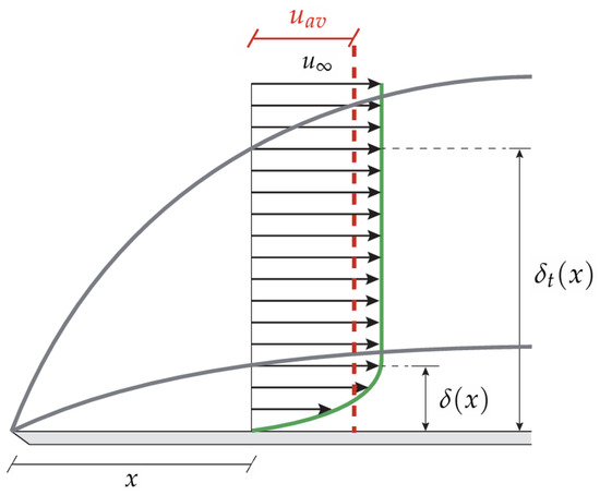
Figure 4. The velocity profile within the thermal boundary layer for low-$Pr$ fluids.

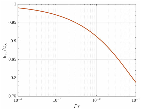
Figure 5. The distribution of $u_{av}/u_{\infty }$ versus the Prandtl number.

Accordingly, for fluids having a small non-zero value of the Prandtl number, a weak dependence on $\nu$ should be introduced. In this case Equation (19) becomes

$${\displaystyle \frac{{\delta }_t}{x}}\propto {\displaystyle \frac{\alpha }{x{u}_{\infty }}},{\displaystyle \frac{{\delta }_t}{x}}\propto {\displaystyle \frac{\nu }{\alpha }}$$

(24)

which means

$${\displaystyle \frac{{\delta }_t}{x}}\propto {\displaystyle \frac{1}{Pe}},{\displaystyle \frac{{\delta }_t}{x}}\propto Pr$$

(25)

where the second proportionality relationship simply plays a refining role, the main phenomenology being already included in the Péclet number. Therefore, it is reasonable to assume that the first dependence in Equation (25) is the same as that for $Pr\to 0$. On the other hand, the second dependence in Equation (25) should be expressed through a weak corrective function $f\left(Pr\right)$, directly proportional to the Prandtl number and constructed to preserve the direct proportionality of ${\delta }_t/x$ on $\alpha$. Hence, we have

$${\displaystyle \frac{{\delta }_t}{x}}\sim {\displaystyle \frac{1}{P{e}^{\sigma }}}(0<\sigma <1),{\displaystyle \frac{{\delta }_t}{x}}\sim f\left(Pr\right)$$

(26)

Combining Equation (26) with Equation (15) and taking into account the definition of the Nusselt number, we obtain

$$Nu\sim A\left(Pr\right)P{e}^{\sigma }(0<\sigma <1)$$

(27)

where $A\left(Pr\right)=1/f\left(Pr\right)$ is a weak inverse function of the Prandtl number, as displayed in Figure 1, consistently with the Sparrow–Gregg correlation reported in Equation (3), where the exponent $\sigma$ is found to be equal to $1/2$.

Following the same reasoning applied in the discussion of Equation (17), the exponent $\sigma$ in Equation (27), directly derived from Equation (26), is expected to be $1/2$, as the thickness of the thermal boundary layer directly derives from the thickness of the velocity boundary layer, which is inversely proportional to $R{e}^{1/2}$. Therefore, since the Péclet number—defined as the product between the Reynolds and Prandtl numbers—is the only relevant dimensionless group, it must be raised to the $1/2$ power. Moreover, comparing the distributions represented in Figure 1 and Figure 5, it is evident that the shape of $A\left(Pr\right)$—which increases asymptotically as $Pr\to 0$—directly derives from the distribution of $u_{av}/u_{\infty }$.

5. Conclusions

Using a new phenomenological boundary layer approach based solely on qualitative physical arguments, the direct dependence of the Nusselt number on the Reynolds and Prandtl numbers for forced convection heat transfer problems is derived, without employing scaling analyses or solving the governing equations.

Once a power law functional dependence is assumed, it has been demonstrated that for moderate-to-high-$Pr$ fluids, the exponent $\gamma$ of the Reynolds number should be related to the exponent $\lambda$ of the Prandtl number by the relationship: $0<\lambda <\gamma <1$.

Conversely, it has been shown that, for low-$Pr$ fluids, exponents $\gamma$ and $\lambda$ are equal—since the phenomenon is fully described by the Péclet number—and that each is less than unity. In this case, the introduction of a coefficient $A\left(Pr\right)$, weakly inversely dependent on the Prandtl number, has also been discussed to account for the residual effects of the fluid’s kinematic viscosity.

References

- Murshed, S.S.; De Castro, C.N. A critical review of traditional and emerging techniques and fluids for electronics cooling. Renew. Sustain. Energy Rev. 2017, 78, 821–833. [Google Scholar] [CrossRef]
- Marzouk, S.A.; Abou Al-Sood, M.M.; El-Said, E.M.; Younes, M.M.; El-Fakharany, M.K. A comprehensive review of methods of heat transfer enhancement in shell and tube heat exchangers. J. Therm. Anal. Calorim. 2023, 148, 7539–7578. [Google Scholar] [CrossRef]
- Santos, A.A.D.L.; Leal, G.F.; Marques, M.R.; Reis, L.C.C.; Junqueira, J.R.D.J.J.; Macedo, L.L.; Corrêa, J.L.G. Emerging drying technologies and their impact on bioactive compounds: A systematic and bibliometric review. Appl. Sci. 2025, 15, 6653. [Google Scholar] [CrossRef]
- Barmavatu, P.; Deshmukh, S.A.; Das, M.K.; Arabkoohsar, A.; García-Merino, J.A.; Rosales-Vera, M.; Sunil Dsilva, R.; Ramalinga Viswanathan, M.; Gaddala, B.; Sikarwar, V.S. Heat transfer characteristics of multiple jet impingements using graphene nanofluid for automobile industry application. Therm. Sci. Eng. Prog. 2024, 55, 102993. [Google Scholar] [CrossRef]
- Agbevanu, K.T.; Debrah, S.K.; Arthur, E.M.; Shitsi, E. Liquid metal cooled fast reactor thermal hydraulic research development: A review. Heliyon 2023, 9, e16985. [Google Scholar] [CrossRef] [PubMed]
- Lorenzin, N.; Abanades, A. A review on the application of liquid metals as heat transfer fluid in Concentrated Solar Power technologies. Int. J. Hydrogen Energy 2016, 41, 6990–6995. [Google Scholar] [CrossRef]
- Deng, Y.; Jiang, Y.; Liu, J. Low-melting-point liquid metal convective heat transfer: A review. Appl. Therm. Eng. 2021, 193, 117021. [Google Scholar] [CrossRef]
- Heinzel, A.; Hering, W.; Konys, J.; Marocco, L.D.; Litfin, K.; Müller, G.; Pacio, J.; Schroer, C.; Stieglitz, R.; Stoppel, L.; et al. Liquid metals as efficient high-temperature heat-transport fluids. Energy Technol. 2017, 5, 1026–1036. [Google Scholar] [CrossRef]
- Qin, C.; Song, P.; Sun, X.; Wang, R.; Wei, M.; Mao, M. Actuation technique of liquid metal in thermal management: A review. Appl. Therm. Eng. 2024, 248, 123290. [Google Scholar] [CrossRef]
- Gebhart, B. Heat Transfer; McGraw-Hill: New York, NY, USA, 1961. [Google Scholar]
- Incropera, F.P.; DeWitt, D.P.; Bergman, T.L.; Lavine, A.S. Fundamentals of Heat and Mass Transfer, 5th ed.; Wiley: New York, NY, USA, 1996. [Google Scholar]
- Kreith, F.; Manglik, R.M.; Bohn, M.S. Principles of Heat Transfer, 8th ed.; Cengage Learning: Stamford, CT, USA, 2017. [Google Scholar]
- Blasius, H. Grenzschichten in Flüssigkeiten mit kleiner Reibung. Z. Math. Phys. 1908, 56, 1–37. [Google Scholar]
- Pohlhausen, K. Der Wärmeübergang zwischen festen Körpern und Flüssigkeiten mit kleiner Reibung und kleiner Wärmeleitung. Z. Angew. Math. Mech. 1921, 1, 115–121. [Google Scholar] [CrossRef]
- Schlichting, H.; Gersten, K. Boundary-Layer Theory, 9th ed.; Springer: Berlin/Heidelberg, Germany, 2017. [Google Scholar]
- Saldana, M.; Gallegos, S.; Gálvez, E.; Castillo, J.; Salinas-Rodríguez, E.; Cerecedo-Sáenz, E.; Toro, N. The Reynolds number: A journey from its origin to modern applications. Fluids 2024, 9, 299. [Google Scholar] [CrossRef]
- Tamburrino, A.; Niño, Y. The universal presence of the Reynolds number. Fluids 2025, 10, 117. [Google Scholar] [CrossRef]
- Sparrow, E.M.; Gregg, J.L. Details of Exact Low Prandtl Number Boundary-Layer Solutions for Forced and for Free Convection; NASA Memorandum NASA-MEMO-2-27-59E; National Aeronautics and Space Administration: Washington, DC, USA, 1959.
- Morgan, G.W.; Pipkin, A.C.; Warner, W.H. On heat transfer in laminar boundary-layer flows of liquids having a very small Prandtl number. J. Aerosp. Sci. 1958, 25, 173–180. [Google Scholar] [CrossRef]
- Bejan, A. Convection Heat Transfer; Wiley: New York, NY, USA, 1984. [Google Scholar]
- Churchill, S.W.; Ozoe, H. Correlations for laminar forced convection in flow over an isothermal flat plate and in developing and fully developed flow in an isothermal tube. J. Heat Transf. 1973, 95, 416–419. [Google Scholar] [CrossRef]
- Gnielinski, V. Berechnung mittlerer Wärme- und Stoffübergangskoeffizienten an laminar und turbulent überströmten Einzelkörpern mit Hilfe einer einheitlichen Gleichung. Forsch. Ingenieurwesen A 1975, 41, 145–153. [Google Scholar] [CrossRef]
- Ahmed, G.R.; Yovanovich, M.M. Analytical method for forced convection from flat plates, circular cylinders, and spheres. J. Thermophys. Heat Transf. 1995, 9, 516–523. [Google Scholar] [CrossRef]
- Lienhard, J.H. Heat transfer in flat-plate boundary layers: A correlation for laminar, transitional, and turbulent flow. J. Heat Transf. 2020, 142, 061805. [Google Scholar] [CrossRef]
- Zhao, J.; Zhu, J.; Xu, Y.; Li, Y. New generalized expressions for forced convective heat transfer coefficients across the flat plate. Appl. Therm. Eng. 2025, 258, 124688. [Google Scholar] [CrossRef]
Disclaimer/Publisher’s Note: The statements, opinions and data contained in all publications are solely those of the individual author(s) and contributor(s) and not of MDPI and/or the editor(s). MDPI and/or the editor(s) disclaim responsibility for any injury to people or property resulting from any ideas, methods, instructions or products referred to in the content. |
© 2025 by the authors. Licensee MDPI, Basel, Switzerland. This article is an open access article distributed under the terms and conditions of the Creative Commons Attribution (CC BY) license.