Machine Learning-Based Material Thickness and Type Classification via Scattering Parameters

Abstract

The precise determination of material type and thickness is of major significance in non-destructive testing, quality assurance, and materials science, as it influences the functionality, reliability, and performance of materials in engineering applications. This study proposes a methodology for the classification of material thickness and type through the analysis of scattering parameters within the 8–12 GHz frequency range. A database was created, encompassing real, imaginary, and dB values of reflection and transmission parameters for nine real-world materials with thicknesses ranging from 1 to 10 mm. This study addressed two main classification tasks, namely material thickness and material type. A variety of training–testing splits were employed in conjunction with 10-fold cross-validation to facilitate a comparison of classifier performance. In the material type classification, incorporating multiple thickness levels of each material enabled the model to distinguish materials with similar reflection characteristics more accurately, thereby enhancing discrimination performance. The results showed that Fine KNN consistently achieved 100% accuracy in thickness classification, while Quadratic SVM achieved 100% accuracy in material type classification, even when utilising only three thickness levels. Furthermore, the 90% training–10% testing split yielded the highest performance in thickness classification, whereas the optimal data split for material type classification differed across classifiers. Overall, this study demonstrates that the combination of scattering parameters and machine learning serves as a reliable and efficient approach for non-destructive material characterization.

1. Introduction

The accurate determination of material type and thickness is a fundamental requirement in materials science, non-destructive testing (NDT), and quality assurance [1]. These parameters directly affect the electromagnetic, mechanical, and structural properties of materials. Consequently, they play a decisive role in functionality, reliability, and performance across a wide range of applications, from electronic devices [2] to aerospace engineering [3], defense technologies [4], and civil engineering [5]. In modern industry, rapid, precise, and non-destructive material characterization has become critical for product safety, performance optimization, and defect prevention. For this reason, microwave- and radio-frequency-based methods have gained increasing attention in recent years, as they offer fast, contactless, and reliable evaluation without damaging the material [6].

A wide variety of methods have been proposed in the literature for material characterization. Conventional techniques include optical measurements, mechanical testing, and ultrasonic inspection [7]. However, many of these methods require direct contact, involve complex experimental setups, or are limited in practical use due to long measurement times. Microwave-based approaches, particularly those utilising scattering parameters (S-parameters), have emerged as prominent techniques for determining the dielectric properties of materials [8]. Reflection (S₁₁) and transmission (S₂₁) coefficients provide valuable information about the dielectric constant, thickness, and structural characteristics of a material. Conventional electromagnetic NDT methods often rely on inversion-based retrieval of dielectric properties from measured S-parameters [9,10,11]. Such approaches require additional modeling and calibration steps, which may introduce uncertainty. Direct use of S-parameter responses avoids these intermediate steps and enables data-driven exploitation of the full spectral information for classification tasks. Recently, the evaluation of high-dimensional spectral data derived from these parameters using machine learning algorithms has enabled highly accurate classification of critical parameters such as material type and thickness [12].

Several approaches have been reported in the literature. For example, Hien and Hong (2021) performed thickness classification by employing deep neural networks (DNNs) and support vector machines (SVMs) using dielectric constants derived from S-parameters [13]. However, their method requires an additional transformation step rather than using the S-parameters directly. Harrsion et al. (2018) employed a microwave sensor array to differentiate material types by classifying resonance responses with machine learning algorithms [14]. This study was limited in terms of material diversity and did not address thickness classification. Tan and Yoon (2024) used simulation-based scattering data to estimate the thickness of fat and muscle layers in the human body through regression models, but the study focused only on continuous thickness prediction and did not include material type classification [15]. In a broader perspective, Hinderhofer et al. (2023) reviewed strategies for analyzing scattering data with machine learning, discussing feature extraction and classification techniques [16]. Yildirim et al. (2024) further proposed a multi-task approach that enables both classification and parameter estimation from scattering data [17]. These studies collectively highlight the growing significance of integrating scattering parameters with machine learning. Despite these studies, a clear experimental benchmark that directly exploits broadband S-parameter responses for simultaneous material type and thickness classification using standard machine learning models remains lacking. Nevertheless, most existing studies have been conducted on a limited number of materials or within narrow thickness ranges. In addition, many studies have focused on a single issue, such as either thickness or material type. From a broader perspective, the proposed approach aligns with recent trends in machine learning-based sensing pipelines, where raw sensor signals are directly mapped to high-level decisions under real-time constraints. Similar data-driven paradigms have been explored in air-quality prediction using mobility-assisted sensing [18] and real-time intelligent transportation systems [19]. In this context, the present work extends such sensing pipelines to the domain of microwave nondestructive testing by leveraging broadband S-parameter measurements.

In this study, we aim to address these gaps by directly utilising scattering parameters within the 8–12 GHz frequency range to classify both material thickness and material type. Nine different materials, including alumina, mica, wood, polymethyl methacrylate (PMMA), polytetrafluoroethylene (PTFE), flame-retardant epoxy laminate (FR4), lead glass, gold, and copper, were evaluated, and a comprehensive database was constructed covering thicknesses from 1 to 10 mm. A total of 1001 frequency points were employed in this range, providing high-resolution spectral data. Recent studies in the field of classification and super-resolution demonstrate that advanced artificial intelligence techniques offer significant advantages in processing data containing high-dimensional spectral information [20]. Reflection (S₁₁) and transmission (S₂₁) coefficients in their real, imaginary, and dB forms were considered as features. Various training–testing ratios (90/10, 80/20, 70/30, 60/40, and 50/50) and 10-fold cross-validation were used to evaluate the performance of several machine learning classifiers, including support vector machines (SVMs), k-nearest neighbours (KNNs), ensemble methods (EM), neural networks (NNs), decision trees (DTs), naive Bayes (NB), and discriminant analysis (DA). The results demonstrated that Fine KNN consistently achieved 100% accuracy in thickness classification, while Quadratic SVM achieved 100% accuracy in material type classification. Remarkably, the same high performance was maintained even when only three different thickness values were used simultaneously.

In this study, the real, imaginary, and dB components of S₁₁ and S₂₁ were fed directly into machine learning models, thereby eliminating the accumulation of conversion errors associated with approaches requiring the calculation of intermediate quantities such as the dielectric constant, and presenting a simpler, more reliable method. Such conversion-based approaches are known to be sensitive to phase ambiguity and measurement-related effects. In particular, when the sample thickness corresponds to integer multiples of half-wavelengths, the reflection coefficient S₁₁ approaches zero, leading to artificial discontinuities in the retrieved permittivity values [21]. In addition, connector losses, air gaps, and sample placement inaccuracies may further contribute to error accumulation during inversion-based retrieval.

While most studies focus on a single problem, this study addresses both thickness and type classification together and comparatively using the same data collection protocol, strengthening the consistency of the results within the studied materials and experimental configuration. The high-resolution database, comprising nine different materials and ten thickness ranges, overcomes the limitations of limited material diversity and narrow thickness ranges in the literature, thereby increasing the model’s discriminative power within the considered material set. Furthermore, evaluating the classification using different training–test splits of the dataset and cross-validation increases the reliability and robustness of the results. The findings demonstrate that the high performance achieved in both classification tasks confirms the reliability of the S-parameter spectrum as a discriminant. This feature makes the work practical for rapid and non-contact quality assurance in NDT applications, while also proving the effectiveness of the direct S-parameter–ML link in microwave-based material characterization. Furthermore, the proposed approach can be extended towards integration into production lines, validation with different measurement setups, and continuous thickness estimation or multi-task learning. Thus, this work demonstrates the potential transferability of the proposed methodology, which can be further investigated for different material families and experimental conditions in future studies.

The remainder of this article is organized as follows: Section 2 presents the overall framework of this study and the data acquisition method used for machine learning. Section 3 describes the machine learning-based classification methods applied and the results obtained for thickness and material type classification. Finally, Section 4 discusses the conclusions and implications of the findings.

2. Materials and Methods

The methodological flow chart for this study is provided in Figure 1. In the first step, the real, imaginary, and dB components of the reflection (S₁₁) and transmission (S₂₁) coefficients for different materials within a specific frequency and thickness range were obtained. These parameters were organized to create two separate databases for thickness and material type classification. For reproducibility, the feature construction and training workflow followed a deterministic procedure. For thickness classification, each data sample consisted of the frequency index along with the real, imaginary, and dB representations of the S₁₁ and S₂₁ parameters measured at a single thickness level. For material type classification, features were constructed by concatenating the S₁₁ and S₂₁ dB responses corresponding to multiple thickness levels of the same material. The databases were divided into training and test sets at different ratios (90/10, 80/20, 70/30, 60/40, and 50/50) to evaluate the consistency and generalizability of the results. Furthermore, 10-fold cross-validation was applied to reduce the random effects of a single data partition. During the classification stage, a broad set of classifiers belonging to the support vector machine (SVM), k-nearest neighbors (KNN), ensemble methods (bagged/boosted trees), neural networks (NNs), decision trees (DTs), naive Bayes (NB), and discriminant analysis (DA) families were used, and the obtained performances were compared.

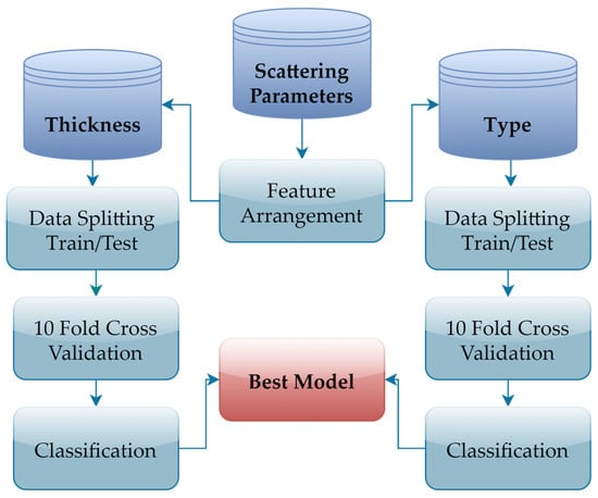
Figure 1. Methodological workflow of this study.

2.1. Scattering Parameters

S-parameters are fundamental quantities that describe the behavior of electromagnetic waves as they propagate through or are reflected by a network or material. These parameters, widely used in electromagnetic characterization studies, are represented by a two-port network model, as illustrated in Figure 2. In this model, $V_1$ and $V_2$ and $I_1$ and $I_2$ denote the voltage and current variables at the first and second ports, respectively. $Z_{o1}$ and $Z_{o2}$ represent the input and output impedances, while $E_s$ indicates the source voltage of the system.

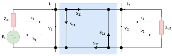
Figure 2. Two-port network representation of scattering parameters.

At microwave frequencies, direct measurement of voltage and current is difficult; therefore, wave variables $a_1$ and $b_1$ and $a_2$ and $b_2$ are employed in the analysis, where $a$ represents the incident wave and $b$ represents the reflected wave. The relationship between the wave variables and the voltage–current quantities is given in Equation (1) [22]:

$$V_n=\sqrt{Z_0}\left(a_n+b_n\right), I_n={\displaystyle \frac{1}{\sqrt{Z_0}}}\left(a_n-b_n\right), n=1, 2$$

(1)

For a two-port network, the scattering (S) parameters are defined in terms of wave variables as expressed in Equation (2).

$$\left[\begin{array}{c}{b}_1\\ b_2\end{array}\right]=\left[\begin{array}{cc}{S}_{11}& S_{12}\\ S_{21}& S_{22}\end{array}\right]\left[\begin{array}{c}{a}_1\\ a_2\end{array}\right]$$

(2)

In this matrix form, ${\mathrm{S}}_{11}$ and ${\mathrm{S}}_{22}$ correspond to the reflection coefficients, while ${\mathrm{S}}_{12}$ and ${\mathrm{S}}_{21}$ represent the transmission coefficients. These parameters are directly measurable at microwave frequencies and, being complex quantities, are typically expressed in terms of magnitude and phase.

S-parameters possess several properties useful in circuit analysis. According to the reciprocity condition, ${\mathrm{S}}_{21}={\mathrm{S}}_{12}$, and for a symmetric network, ${\mathrm{S}}_{11}={\mathrm{S}}_{22}$. Therefore, symmetric networks are also reciprocal. In the present study, only ${\mathrm{S}}_{11}$ and ${\mathrm{S}}_{21}$ parameters were utilised. The measurements of these parameters were performed using an Agilent E5071C Vector Network Analyzer (VNA) manufactured by Keysight Technologies (Santa Rosa, CA, USA) with WR90 and WR102 waveguides. System calibration was carried out using the Thru–Reflect–Line (TRL) calibration method due to the waveguide-based measurement configuration. The WR90 and WR102 waveguides had cross-sectional dimensions of 22.86 × 10.16 mm and 25.91 × 12.95 mm, respectively. The samples were mounted using custom-designed holders matched to the corresponding waveguide dimensions, ensuring stable placement and complete coverage of the waveguide cross-section during measurements. To minimize environmental and moisture-related variability, all samples were conditioned prior to measurements and stored in a desiccator until testing. Measurements were conducted in an anechoic environment to reduce external electromagnetic interference. The laboratory temperature and relative humidity were monitored and maintained at 23 ± 2 °C and approximately 45%, respectively. The scattering parameters were measured for nine different materials: alumina, mica, wood, PMMA, PTFE, FR4, lead glass, gold, and copper. These materials were selected to represent a broad spectrum of electromagnetic properties, ranging from highly conductive metals to low-loss dielectrics. Hence, the constructed database comprehensively reflects the S-parameter responses of materials with diverse electromagnetic properties.

2.2. Datasets Construction

In this study, the frequency range of 8–12 GHz was divided into 1001 discrete points, and for each frequency value, the real and imaginary components of the reflection (S₁₁) and transmission (S₂₁) coefficients were obtained for ten different thicknesses ranging from 1 mm to 10 mm in 1 mm increments. The use of 1001 frequency points over the 8–12 GHz range provides a frequency resolution of approximately 4 MHz, which is sufficient to capture the spectral variations of the measured S-parameters within the employed waveguide configurations. Since the measurements are directly performed in the frequency domain using a vector network analyzer, classical time-domain aliasing effects do not arise. The selected frequency resolution, therefore, represents a balance between spectral detail and computational efficiency. The obtained complex-valued scattering parameters were reformulated in terms of magnitude and decibel (dB) representations using their real and imaginary components, as shown in Equation (3):

$$S_{mn}^{\left(dB\right)}=20\times {\log }_{10}\left(\sqrt{{\left[Re\left(S_{mn}\right)\right]}^2+{\left[Im\left(S_{mn}\right)\right]}^2}\right),\hspace{1em}\hspace{1em}m,n\in \left\{1,2\right\}$$

(3)

The mean and standard deviation values of the materials included in the database are presented in Table 1. As can be seen, subtle differences are observed in the real, imaginary, and dB components of both the reflection and transmission coefficients for each material. These data were subsequently organized for two separate classification problems.

Table 1. Mean ± standard deviation of electromagnetic parameters (S₁₁ and S₂₁) included in the datasets.

Material	Re (S11)	Im (S11)	Re (S21)	Im (S21)	S11 (dB)	S21 (dB)
FR4	−0.0462 ± 0.1756	0.4724 ± 0.1045	−0.017 ± 0.1595	0.0028 ± 0.1618	−6.1198 ± 1.9621	−13.1446 ± 1.6125
PMMA	−0.0584 ± 0.1516	0.4685 ± 0.0886	−0.0233 ± 0.1494	0.0027 ± 0.1519	−6.3079 ± 1.8279	−13.4951 ± 0.9994
PTFE	−0.0613 ± 0.1405	0.4629 ± 0.0829	−0.029 ± 0.1458	0.0011 ± 0.1492	−6.4522 ± 1.7787	−13.5858 ± 0.6876
Alumina	−0.0931 ± 0.2148	0.5169 ± 0.1173	−0.0126 ± 0.1494	0.0059 ± 0.151	−5.1525 ± 2.067	−14.139 ± 2.4914
Cu	−0.047 ± 0.2828	0.5366 ± 0.1398	0.001 ± 0.0219	0.0025 ± 0.0208	−4.3314 ± 1.5761	−30.5437 ± 1.2518
Gold	−0.047 ± 0.2828	0.5366 ± 0.1398	0.001 ± 0.0219	0.0025 ± 0.0208	−4.3314 ± 1.5761	−30.5437 ± 1.2518
Lead Glass	−0.0423 ± 0.1934	0.4725 ± 0.1205	−0.0153 ± 0.1623	0.0031 ± 0.163	−6.0491 ±2.216	−13.1948 ± 1.9812
Mica	−0.0423 ± 0.1934	0.4725 ± 0.1204	−0.0153 ± 0.1623	0.003 ± 0.163	−6.0494 ± 2.2155	−13.1935 ± 1.9814
Wood	−0.059 ± 0.1246	0.4565 ± 0.0779	−0.0338 ± 0.1308	−0.0045 ± 0.1369	−6.6407 ± 1.7357	−14.3637 ± 0.6321

In the database constructed for material thickness classification, the target variable corresponds to the thickness values of the samples. The employed feature vector is presented in Equation (4). Accordingly, a dataset with a dimension of 7 × 90,090 was obtained, and the classification procedure for material thickness estimation was subsequently carried out using this dataset.

$${Features}_{Thickness}=\left[freq, Re\left(S_{11}\right), Im\left(S_{11}\right), Re\left(S_{21}\right), Im\left(S_{21}\right), S_{11}^{\left(dB\right)},S_{21}^{\left(dB\right)}\right]$$

(4)

In the database constructed for material type classification, the target variable represents the different material categories. Each record in this database contains the reflection and transmission coefficients, expressed in decibels (dB), corresponding to ten distinct thickness values (1–10 mm) of the same material. Accordingly, the feature vector consists of the frequency information along with the dB representations of the S₁₁ and S₂₁ parameters for each thickness level, as shown in Equation (5).

$${Features}_{Type}=\left[freq, S_{11,1}^{\left(dB\right)},S_{21,1}^{\left(dB\right)},S_{11,2}^{\left(dB\right)},S_{21,2}^{\left(dB\right)},\cdots , S_{11,10}^{\left(dB\right)},S_{21,10}^{\left(dB\right)}\right]$$

(5)

The structure presented in Equation (3) enables the direct use of dB values derived from reflection and transmission parameters measured at different thickness levels, allowing machine learning models to distinguish the electromagnetic response profiles of materials. The resulting database has a total dimension of 21 × 9009. It should be noted that the 1001 frequency points are not treated as independent samples; instead, they collectively form a single feature vector corresponding to one measurement instance. No manual normalization or feature scaling was applied prior to model training. For distance- and kernel-based classifiers, internal standardization was automatically performed by the MATLAB 2024a Classification Learner environment (developed by MathWorks, Natick, MA, USA) during training and validation. Both magnitude-based and logarithmic (dB) representations of the S-parameters were included as complementary features. Although mathematically related, these representations emphasize different aspects of the spectral response and were therefore jointly considered rather than treated as redundant. The dataset was constructed to ensure comparable representation across material types and thickness classes, avoiding severe class imbalance.

2.3. Classification Process and Performance Analysis

After organizing the data for two separate classification problems, different training–testing split ratios (90/10, 80/20, 70/30, 60/40, and 50/50) were applied to train machine learning-based classification models and to evaluate their performance under various data distribution scenarios. Additionally, the 10-fold cross-validation procedure, illustrated in Figure 3, was employed during the training phase to minimize random effects that may arise from a single data split and to enhance the reliability of the performance assessment. In this method, the training set is divided into ten parts, and in each iteration, one part is set aside for validation, while the remaining nine parts are used for training. The final accuracy is calculated as the average of the ten iterations.

Figure 3. Workflow of the 10-fold cross-validation method.

In this study, seven fundamental classifier algorithms (SVM, KNN, ensemble methods (bagged/boosted trees), NN, DT, NB, and DA) and numerous different sub-variants (e.g., Quadratic SVM, Fine KNN) for each were tested to determine the highest accuracy values within the scope of supervised machine learning. Among these methods, SVM is a powerful algorithm that aims to determine the maximum margin between classes by mapping data points to a high-dimensional space [23]. For non-linear data, classification performance can be improved by using kernel functions. In this study, the Quadratic SVM method in particular provided the highest accuracy in material type classification. The KNN method is a straightforward yet efficacious algorithm that determines the class of examples based on neighbourhood relationships [24]. Achieving high accuracy rates is especially feasible in the context of uncomplicated data distributions. The Fine KNN variant employed in this study yielded the most accurate results in all data partition ratios in thickness classification. The objective of ensemble methods is to create a powerful prediction model by combining multiple weak classifiers (e.g., decision trees) [25]. The bagged tree method reduces variance through bootstrap sampling and majority voting, while the boosted tree method increases model accuracy by assigning greater weight to misclassified examples. Artificial neural networks (NNs) are a class of machine learning algorithms inspired by the biological neural systems in the human brain. They are capable of learning complex nonlinear relationships due to their multi-layered structure [26]. Decision trees (DTs) are an intuitive method that determines the class decision by dividing the data into branches through the sequential evaluation of features [27]. Thanks to its simple structure, it is highly interpretable, but when used alone, it is a method that is sensitive to noise. The naive Bayes (NB) classifier is a probabilistic method based on Bayes’ theorem that assumes conditional independence between features [28]. It offers a computationally inexpensive, fast solution, particularly for high-dimensional datasets. In the discriminant analysis (DA) method, linear (LDA) or quadratic (QDA) boundary functions that distinguish between classes are used [29]. This method yields highly successful results when the data classes are close to a normal distribution. The classifier variants and their hyperparameters used in this study were selected based on the standard default configurations suggested by the MATLAB Classification Learner tool. These settings were accepted as a starting point and ensure a fair and reproducible comparison between models.

The accuracy metric was utilised to evaluate and compare the classification performance since the dataset was balanced, meaning that each class contained an equal number of samples. Accuracy is defined as the proportion of correctly classified samples to the total number of samples, as presented in Equation (6).

$$Accuracy={\displaystyle \frac{Number of correct predictions}{Total number of predictions}}$$

(6)

The machine learning analyses were conducted using a personal computer equipped with an Intel Core i5-11400H central processing unit (CPU) manufactured by Intel Corporation (Santa Clara, CA, USA) operating at 2.70 GHz, 64 GB of random-access memory (RAM), and the Windows 11 (Microsoft Corporation, Redmond, WA, USA) operating system. The MATLAB R2024a environment was utilised for model training, validation, and performance evaluation.

3. Results

In this section, the results pertaining to material thickness and type classification are presented in separate tables according to the classification model families utilised. The tables present the validation and test accuracy values obtained for each model at varying training-test split ratios of the dataset. Firstly, as illustrated in Table 2, a comparison is made of the performance of KNN-based models utilised in material thickness classification. In addition to classification accuracy, computational efficiency is evaluated through prediction speed metrics. In this study, one observation corresponds to a complete feature vector extracted from the full S-parameter spectrum (8–12 GHz) of a single sample. Accordingly, the reported prediction speeds (observations/s) represent the number of complete samples that can be classified per second. Considering a simple inspection scenario involving one to several parts per second, the achieved classification speeds are sufficient for real-time operation. It should also be noted that data acquisition using a vector network analyzer dominates the overall processing time, while feature construction and classification introduce negligible additional latency. In this study, repeated random data splitting was not employed. Instead, 10-fold cross-validation was applied exclusively on the training set, where the data were partitioned into ten folds, and each fold was used once for validation. The validation accuracy values reported in Table 2, Table 3, Table 4, Table 5, Table 6, Table 7, Table 8, Table 9, Table 10 and Table 11 correspond to the mean accuracy obtained across these folds. After model selection, the trained classifiers were evaluated on an independent test set that was not used during training or validation, and the resulting performance was reported as test accuracy.

Table 2. Thickness classification performance of KNN-based models.

KNN-Based Models	Split Rate (90/10)		Split Rate (80/20)		Split Rate (70/30)		Split Rate (60/40)		Split Rate (50/50)
	Val. Acc.%	Test Acc.%	Val. Acc.%	Test Acc.%	Val. Acc.%	Test Acc.%	Val. Acc.%	Test Acc.%	Val. Acc.%	Test Acc.%
Fine	100	100	100	100	100	100	100	100	100	100
Weighted	100	100	100	100	100	100	100	100	100	100
Medium	100	100	100	100	99.9	99.9	99.8	99.9	99.3	99.7
Cubic	100	100	100	100	99.9	99.9	99.7	99.9	99.2	99.5
Cosine	99.8	99.9	99.6	99.7	99.5	99.6	99.2	99.4	98.3	98.8
Coarse	82.1	86.2	78.1	81.6	73.4	77.6	67.5	71.3	62.7	64.8

Table 3. Thickness classification performance of SVM-based models.

SVM-Based Models	Split Rate (90/10)		Split Rate (80/20)		Split Rate (70/30)		Split Rate (60/40)		Split Rate (50/50)
	Val. Acc.%	Test Acc.%	Val. Acc.%	Test Acc.%	Val. Acc.%	Test Acc.%	Val. Acc.%	Test Acc.%	Val. Acc.%	Test Acc.%
Fine Gaussian	99.9	99.9	99.9	99.9	99.8	99.8	99.7	99.8	99.4	99.5
Cubic	98	97.6	98.4	96	98.5	97.4	98.5	98.8	98.2	97.3
Medium Gaussian	86.9	87.7	85.8	85.9	84.3	85.5	82.8	84.8	79.6	84.8
Quadratic	69.3	68.7	71	70.9	72.9	74.6	72.7	72.2	75.8	76.3
Coarse Gaussian	29	29.2	28.6	29	28.1	29.1	26.3	26.8	26.3	27.2
Linear	15.9	16	15.4	15.7	15.4	15.5	15.5	15.5	16.2	16.3
Efficient Linear	14.7	15.4	14.3	14.7	15.1	14.6	14.7	14.9	14.6	14.5

Table 4. Thickness classification performance of NN models.

NN-Based Models	Split Rate (90/10)		Split Rate (80/20)		Split Rate (70/30)		Split Rate (60/40)		Split Rate (50/50)
	Val. Acc.%	Test Acc.%	Val. Acc.%	Test Acc.%	Val. Acc.%	Test Acc.%	Val. Acc.%	Test Acc.%	Val. Acc.%	Test Acc.%
Wide	98.8	99.1	98.7	99.1	98.9	99.5	98.8	98.5	98.7	98.5
Medium	85.8	82.4	84.4	84.5	85.7	89.1	85.5	86.8	86.2	88
Trilayered	80.7	84.8	77.6	71.5	78.5	76	80.3	86.2	79.3	81.1
Bilayered	74.8	71.1	73.7	68	81.8	67.7	74.8	72.7	71.8	74.8
Narrow	62.7	60.5	59.3	68.1	59.1	52.5	57.4	57.4	57.7	59.3

Table 5. Thickness classification performance of ensemble methods.

EM-Based Models	Split Rate (90/10)		Split Rate (80/20)		Split Rate (70/30)		Split Rate (60/40)		Split Rate (50/50)
	Val. Acc.%	Test Acc.%	Val. Acc.%	Test Acc.%	Val. Acc.%	Test Acc.%	Val. Acc.%	Test Acc.%	Val. Acc.%	Test Acc.%
Subspace KNN	100	100	100	100	100	100	100	100	100	100
Bagged Trees	99.9	99.9	99.9	99.9	99.9	99.9	99.8	99.9	99.8	99.9
Boosted Trees	31.8	32.1	31.7	32.4	32.3	31.7	32.3	32.8	31.9	32.3
RUS Boosted Trees	29.4	30.4	29	31.6	29.6	30.7	29.6	28.9	28.8	28.6
Subspace Discriminant	12.3	12.4	12.6	12.9	12.8	12.6	13.5	13.4	13	13

Table 6. Thickness classification performance of DT, NB, and DA-based classifiers.

DT-, NB-, and DA-Based Models	Split Rate (90/10)		Split Rate (80/20)		Split Rate (70/30)		Split Rate (60/40)		Split Rate (50/50)
	Val. Acc.%	Test Acc.%	Val. Acc.%	Test Acc.%	Val. Acc.%	Test Acc.%	Val. Acc.%	Test Acc.%	Val. Acc.%	Test Acc.%
Fine Tree	48.2	49	47.6	49.2	48.1	48.7	48.4	47.1	47.9	47.5
Medium Tree	29.2	30.4	28.9	31.2	29.6	30.7	29.6	28.9	28.8	28.6
Coarse Tree	19.1	19.3	19.1	19.1	19.1	19	19.2	19	19	19.2
Kernel Naive Bayes	34	34.5	33.9	34.4	33.1	33	32.4	32.6	33	32.7
Gaussian Naive Bayes	15.4	15.2	15.3	15.3	15.5	15.5	15.7	15.4	15.4	15.4
Quadratic Discriminant	28	28	27.8	28.2	27.7	27.7	27.5	27.9	28.1	28.3
Linear Discriminant	13.6	13.5	13.5	14.1	13.3	13.1	13.3	13.2	13.9	13.9

Table 7. Type classification performance of KNN methods.

KNN-Based Models	Split Rate (90/10)		Split Rate (80/20)		Split Rate (70/30)		Split Rate (60/40)		Split Rate (50/50)
	Val. Acc.%	Test Acc.%	Val. Acc.%	Test Acc.%	Val. Acc.%	Test Acc.%	Val. Acc.%	Test Acc.%	Val. Acc.%	Test Acc.%
Coarse	87	87.2	87.6	86.8	87.5	87.2	87.3	87.4	87.4	87.4
Medium	85.7	85.7	86.5	86	86.3	86	86.7	87	87.8	87.1
Cosine	85.5	84.4	86.4	85.7	86.2	86.9	86.7	86.9	88	86.9
Cubic	85.4	84.3	86.2	85.5	86.1	86.4	86.7	86.9	87.9	87
Weighted	80.3	79.7	81.4	80.4	82.3	81.8	83.2	82.6	84.4	83.7
Fine	79.8	79.2	81.1	80.1	82.3	81.2	83.3	82.5	84.5	83.7

Table 8. Type classification performance of SVM methods.

SVM-Based Models	Split Rate (90/10)		Split Rate (80/20)		Split Rate (70/30)		Split Rate (60/40)		Split Rate (50/50)
	Val. Acc.%	Test Acc.%	Val. Acc.%	Test Acc.%	Val. Acc.%	Test Acc.%	Val. Acc.%	Test Acc.%	Val. Acc.%	Test Acc.%
Quadratic	99.9	100	99.9	100	99.9	100	99.8	100	100	100
Linear	99.8	99.8	99.7	99.7	99.8	99.6	99.8	99.6	99.3	99.5
Cubic	89.6	89	89.1	89	89.1	88.7	89.1	88.8	88.6	89.2
Medium Gaussian	88.1	87.9	88.1	87.4	88.2	88.1	88.3	88.4	88.5	88
Efficient Linear	87.9	88.4	88.2	87.9	88.4	88	88	88.5	88.7	88.3
Coarse Gaussian	87.6	87.4	87.5	87.8	87.4	87.5	87.9	87.4	87.4	87.5
Fine Gaussian	86.7	86.3	87.5	87.2	87.1	87.9	88	87.9	88.1	87.7

Table 9. Type classification performance of NN methods.

NN-Based Models	Split Rate (90/10)		Split Rate (80/20)		Split Rate (70/30)		Split Rate (60/40)		Split Rate (50/50)
	Val. Acc.%	Test Acc.%	Val. Acc.%	Test Acc.%	Val. Acc.%	Test Acc.%	Val. Acc.%	Test Acc.%	Val. Acc.%	Test Acc.%
Wide	96.8	96.3	97.1	97	97	97.5	97	96.7	97	98.5
Medium	96.3	95.4	95.7	96.5	95.4	97.2	95.9	96.3	96.2	94.4
Narrow	90.7	87.9	89.1	87.9	90.5	88	90.5	88.5	91.5	93
Trilayered	88.8	88	87.2	87	91.1	89.7	90	88.5	90.4	87.6
Bilayered	88.4	91	89.3	89	89.3	90.3	89.1	89	92.5	92.5

Table 10. Type classification performance of ensemble methods.

EM-Based Models	Split Rate (90/10)		Split Rate (80/20)		Split Rate (70/30)		Split Rate (60/40)		Split Rate (50/50)
	Val. Acc.%	Test Acc.%	Val. Acc.%	Test Acc.%	Val. Acc.%	Test Acc.%	Val. Acc.%	Test Acc.%	Val. Acc.%	Test Acc.%
Bagged Trees	94.3	94.3	94.7	94.3	93.8	94.6	93.2	93.7	92.7	92.6
Boosted Trees	90.7	90.6	90.7	90.9	90.5	90.6	91.2	90.4	89.7	90.9
RUSBoosted Trees	90.1	90.4	90.1	90.5	90.3	90.8	90.6	89.9	89.9	89.5
Subspace Discriminant	85.3	85.2	85	84.7	85.1	84.1	85.6	85.2	85.5	85.9
Subspace KNN	80.1	79.4	81.5	80.3	82.8	81.9	83.9	82.8	84.7	84.2

Table 11. Type classification performance of DT-, NB-, and DA-based classifiers.

DT-, NB-, and DA-Based Models	Split Rate (90/10)		Split Rate (80/20)		Split Rate (70/30)		Split Rate (60/40)		Split Rate (50/50)
	Val. Acc.%	Test Acc.%	Val. Acc.%	Test Acc.%	Val. Acc.%	Test Acc.%	Val. Acc.%	Test Acc.%	Val. Acc.%	Test Acc.%
Fine Tree	92	91.4	92	91.4	91.3	92	91.3	91.8	90.8	91.3
Medium Tree	90	90.4	90.1	90.4	90.2	90.8	90.5	89.9	89.8	89.5
Coarse Tree	55.5	55.6	55.5	55.6	55.5	55.6	55.5	55.5	55.5	55.6
Kernel Naive Bayes	84.7	84.1	85.1	84.5	84.9	84.5	84.8	84	85.1	85.2
Gaussian Naive Bayes	77.1	77.8	78.1	77.5	79.3	79.7	76.5	76.4	80.8	81.5
Linear Discriminant	86.9	86.9	86.6	86.1	86.6	86.1	86.3	86.4	87.1	86.6

A thorough examination of the performance results of different variants belonging to the KNN family reveals that all models demonstrate high accuracy and consistent prediction speeds. The Fine KNN model was run with a one-neighbour (k = 1) configuration and Euclidean distance metric, achieving an estimation speed of approximately 120,000 observations/second and a training time of 2946.3 s. The compact model size is approximately 8 MB. The Weighted KNN model was implemented in a 10-neighbour configuration (k = 10), with distance-based weighting applied using the squared inverse method. The mean prediction speed was found to be 65,000 observations per second, the training time was 3053.9 s, and the model size was recorded as 8 MB. The Medium KNN model was once more executed in a 10-neighbour configuration (k = 10) and with equal distance weighting; it attained an estimation speed of approximately 69,000 observations per second and a training time of 2953.8 s. The model size is 8 MB. The Cubic KNN model was run with a Minkowski (cubic) distance metric in a 10-neighbour configuration; it demonstrated balanced performance with an average prediction speed of 23,000 observations/second and a training time of 3044.7 s. The model size is approximately 8 MB. The Cosine KNN model was implemented using the cosine distance metric, with an average prediction rate of 2600 observations per second, a training time of 3105.9 s, and a model size of 6 MB. Finally, the Coarse KNN model was run with a 100-neighbour configuration (k = 100), demonstrating lower accuracy but similar processing time compared to other variants, with an approximate prediction speed of 19,000 observations/second and a training time of 2971.6 s.

Table 3 shows the performance of SVM-based models in the thickness classification process.

The Fine Gaussian SVM model was implemented with a Gaussian radial basis function (RBF) kernel to capture non-linear relationships within the feature space. Within the model, the kernel scale has been set to 0.66, and the box constraint level has been set to 1. The one-vs-one strategy has been utilised for multi-class classification, with an average prediction speed of approximately 870 observations per second being achieved. The training time is 2680.9 s, and the compact model size is 10 MB. The cubic SVM model is configured with a cubic kernel function. The kernel scale was automatically determined in the model, and the box constraint level was set to 1. The one-vs-one strategy was applied for multi-class classification operations, and the average prediction speed was measured at approximately 16,000 observations/second, with a training time of 31,831 s. The compact model size is approximately 2 MB. The Medium Gaussian SVM model was configured using the Gaussian RBF kernel function. Within the model, the kernel scale was set to 2.6 and the box constraint level to 1. The one-vs-one strategy was employed for multi-class classification, with the average prediction speed measured at approximately 490 observations/second, the training time at 3027.1 s, and the compact model size at 13 MB. The Quadratic SVM model was configured using a quadratic kernel function. The kernel scale was automatically determined in the model, and the box constraint level was set to 1. The one-vs-one strategy was used for multi-class classification, and the average prediction speed was approximately 5400 observations/second. The training time was 35,544 s, and the compact model size was 8 MB. The coarse Gaussian support vector machine (SVM) model was configured with a Gaussian RBF kernel function, and the kernel scale was set to 11. The box constraint level was set at 1, and the multi-class classification method was implemented as one-vs-one. The mean prediction speed is approximately 250 observations per second, the training time is 6733.4 s, and the compact model size is 36 MB. The Linear SVM model is configured using a linear kernel function. The kernel scale is automatically determined, and the box constraint level is set to 1. The one-vs-one strategy was used for multi-class classification tasks, and the average prediction speed was measured to be approximately 79,000 observations/second. The training time was 23,977 s, and the compact model size was 225 kB. The Efficient Linear SVM model is an optimized SVM structure that uses a linear kernel function. The solver was automatically selected in the model, and the regularisation parameters and regularisation coefficient (λ) were automatically determined. The relative coefficient tolerance (beta tolerance) is 0.0001, and the multi-class classification strategy is set to one-vs-one. The average prediction speed is approximately 97,000 observations/second, the training time is 50,831 s, and the compact model size is 526 kB.

Table 4 shows the performance of NN-based models in the thickness classification process.

The Wide Neural Network model has been constructed with a structure containing a single fully connected layer. The first layer contains 100 neurons, and the ReLU (Rectified Linear Unit) activation function has been used. The iteration limit of the model is set to 1000, and the regularisation coefficient (λ) is set to zero. The average prediction speed is approximately 270,000 observations/second, the training time is 7577.7 s, and the compact model size is measured at 20 kB. The Medium Neural Network model has a structure with a single fully connected layer and 25 neurons. ReLU was used as the activation function, the iteration limit was set to 1000, and the λ was set to zero. The model’s average prediction speed was approximately 310,000 observations/second, the training time was 5257.8 s, and the compact model size was measured at 9 kB. The Trilayered Neural Network model has a multi-layered structure consisting of three fully connected layers. Each of the first, second, and third layers contains 10 neurons, and ReLU was used as the activation function. The iteration limit of the model was set to 1000, the λ was set to zero, and the average prediction speed was approximately 330,000 observations/second. Tthe training time was measured as 8133.8 s, and the model size was 11 kB. The Bilayered Neural Network model has a structure consisting of two fully connected layers. Each of the first and second layers contains 10 neurons, and ReLU was used as the activation function. The iteration limit of the model was set to 1000, and the λ was set to 0. The average prediction speed was measured at approximately 310,000 observations/second, the training time at 6587.4 s, and the model size at 9 kB. The Narrow Neural Network model has a simple structure containing a single fully connected layer. This layer has 10 neurons, and ReLU was chosen as the activation function. The model’s iteration limit was set to 1000, the regularisation coefficient λ was set to 0, and the average prediction rate was measured at 350,000 observations/second, the training time was measured at 4526.6 s, and the model size was measured at approximately 7 kB.

Table 5 presents the performance of ensemble-based models in the thickness classification process.

The Subspace KNN model was created using a subspace-based ensemble learning approach. The nearest neighbors algorithm was used as the base learner in the model, and a structure containing a total of 30 learners was designed. Each learner was trained on a four-dimensional subspace (subspace dimension = 4). The average prediction speed was measured at approximately 11,000 observations/second, the training time was 3467.8 s, and the compact model size was 172 MB. In the Bagged Tree model, which is an ensemble method based on the bootstrap aggregating (bagging) principle, decision trees were used as the base learners, and the final decision structure was created with 30 learners, each trained on different subsamples. The maximum branch (split) count was set to 81,080. The average prediction speed is ~32,000 observations/second, the training time is 3486.9 s, and the compact model size is 17 MB. The boosted tree model is an ensemble learning method based on the AdaBoost (Adaptive Boosting) algorithm. In this model, decision trees were used as the base learners, and a structure was created containing 30 learners, each trained with different weights. The maximum number of branches is set to 20, and the learning rate is set to 0.1. The average prediction speed is measured at ~47,000 observations/second, the training time is 3333.8 s, and the compact model size is approximately 434 kB. In the RUSBoosted (Random Under-Sampling Boosting) Tree model, an ensemble learning method based on the RUSBoost algorithm, decision trees were used as the base learners, and a total of 30 learners were trained. For each tree, the maximum number of splits was set to 20, and the learning rate was set to 0.1. The model’s average prediction speed is ~45,000 observations/second, its training time is 3765.9 s, and its compact model size is approximately 434 kB. The Subspace Discriminant model is an ensemble learning approach based on the subspace method. In this model, discriminant analysis-based classifiers were used as the basic learners. A total of 30 learners were trained, each configured to operate in four-dimensional subspaces (subspace dimension = 4). The average prediction speed was measured at ~25,000 observations/second, the training time was 3375.6 s, and the compact model size was approximately 155 kB.

Table 6 shows the performance of methods based on decision tree, naive Bayes and discriminant analysis. In the Fine Tree model, a classifier belonging to the decision tree family that creates detailed decision boundaries with high branching depth (maximum 100 splits), the Gini diversity index is used as the splitting criterion. The average prediction speed is quite high, at approximately 310,000 observations per second. The training time was recorded as 12.7 s, and the compact model size was approximately 55 kB. The Medium Tree model is structured within the decision tree family with a maximum split limit of 20. The Gini diversity index was again used as the splitting criterion. The model’s average prediction speed was measured at approximately 310,000 observations/second, and the training time was 9.44 s. The compact model size is quite small (~14 kB). The Coarse Tree model has a highly simplified structure, created with a maximum split limit of 4 in the decision tree family. The Gini diversity index was used as the split criterion. The model’s average prediction speed is approximately 300,000 observations/second, and it has a short training time of 8.38 s. The compact model size is only ~6 kB. For the Kernel Naive Bayes model, the average prediction speed was measured at approximately 110 observations/second, the training time was measured at 2940.1 s, and the model size was measured at ~17 MB. For the Gaussian Naive Bayes model, the average prediction speed was measured at approximately 240,000 observations/second, the training time was measured at 15.27 s, and the model size was measured at ~13 kB. The Quadratic Discriminant model adopts the ‘Full covariance structure’ approach, assuming that the covariance matrix of each class may be different. The model’s average prediction speed was measured at approximately 200,000 observations/second, training time was measured at 16.45 s, and model size was measured at approximately 21 kB. In the Linear Discriminant model, the average prediction speed was measured at approximately 220,000 observations/second, training time was measured at 7.27 s, and model size was measured at approximately 7 kB.

In the evaluation of the training–test splits, it was found that the 90/10 split yielded the most consistent and accurate results across a wide range of classifier families. Consequently, this specific split ratio was determined to be the most effective configuration for the thickness classification task and was utilised as the baseline for comparing model speed, size, and training times. Figure 4 shows the validation and test accuracies, along with the prediction speeds, of the most successful models belonging to all classifier families used for material thickness classification. As can be seen from the graphics, it demonstrates that KNN-based models are quite suitable and efficient for material thickness detection applications.

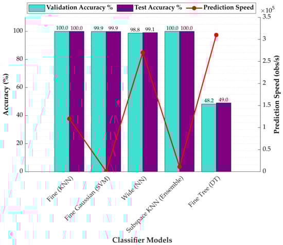
Figure 4. Comparison of the accuracy and prediction speed of the most successful thickness classifiers.

Similar to the thickness classification analysis, the material type classification results obtained from different classifier families are summarized. Since the optimal training–testing split ratio varied across classifiers, the configuration corresponding to each model’s best performance was used to compare prediction speed, model size, and training time.

Table 7 shows the performance of KNN-based models in the material type classification process. Upon examination of the test results for this classification family, it was determined that the most successful method and the highest overall average split ratio were 50/50, respectively. The Coarse KNN model was run with a 100-neighbour (k = 100) configuration using the Euclidean distance metric. Distance weights were assigned as equal, and the average prediction speed was recorded as approximately 15,000 observations/second, with a training time of 22.90 s. The compact model size is approximately 823 kB. The Medium KNN model was run with a 10-neighbour (k = 10) configuration and using the Euclidean distance metric. Distance weights were assigned equally. The model’s average prediction speed was recorded as approximately 18,000 observations/second, the training time was recorded as 21.507 s, and the compact model size was recorded as approximately 823 kB. The Cosine KNN model was run with a 10-neighbour (k = 10) configuration and using the cosine distance metric. The distance weights were set to equal, and the model’s average prediction speed was recorded as approximately 6700 observations/second, the training time was recorded as 24.613 s, and the compact model size was recorded as approximately 823 kB. The Cubic KNN model was run with a 10-neighbour (k = 10) configuration and using the Minkowski (cubic) distance metric. Distance weights were assigned equally. The model’s average prediction speed was recorded as approximately 1300 observations/second, the training time was recorded as 37.173 s, and the compact model size was recorded as approximately 823 kB. The Weighted KNN model was run with a 10-neighbour (k = 10) configuration and using the Euclidean distance metric. Distance weights were assigned using the squared inverse method. The model’s average prediction speed was recorded as approximately 9100 observations/second, the training time was recorded as 26.73 s, and the compact model size was recorded as approximately 823 kB. The Fine KNN model was run using a one-neighbour (k = 1) configuration and the Euclidean distance metric. Distance weights were assigned equally. The model’s average prediction speed was recorded as approximately 19,000 observations/second, the training time as 20.643 s, and the compact model size as approximately 823 kB.

Table 8 shows the performance of SVM-based models in the material type classification process. Analyses of the classifier family showed that the top-performing method achieved flawless classification for all train–test splits, whereas the highest mean accuracy among the remaining methods was obtained at the 60/40 split ratio. The Quadratic SVM model was configured using a quadratic kernel function. The kernel scale was set automatically, the Box constraint value was set to 1, and the one-vs-one encoding method was used for multi-class classification. The model’s prediction speed was recorded at approximately 7600 observations/second, the training time was 102.83 s, and the compact model size was approximately 408 kB. The Linear SVM model was configured with a linear kernel function. The kernel scale was set to automatic, and the Box constraint parameter was set to 1. The one-vs-one encoding approach was applied in multi-class classification, and the model’s prediction speed was recorded as approximately 15,000 observations/second, the training time was recorded as 43.69 s, and the compact model size was recorded as approximately 255 kB. The Cubic SVM model was configured using a cubic kernel function. The kernel scale was set to automatic, and the Box constraint value was set to 1. The one-vs-one coding method was preferred for multi-class classification. The model’s prediction speed is approximately 7000 observations/second, the training time is 104.82 s, and the compact model size is approximately 463 kB. The Medium Gaussian SVM model is configured with a Gaussian (RBF) kernel function. The kernel scale is set to 4.6, and the Box constraint value is set to 1. The one-vs-one encoding method was used for multi-class classification. The model’s prediction speed is approximately 11,000 observations/second, the training time is 15.87 s, and the compact model size is approximately 689 kB. The Efficient Linear SVM model was configured using a linear kernel function. The model solver was automatically determined, and the regularisation and regularisation coefficient (lambda) parameters were also automatically set. The relative coefficient tolerance (beta tolerance) was selected as 0.0001. The one-vs-one strategy was used for multi-class classification. The model’s prediction speed was recorded as approximately 21,000 observations/second, the training time was recorded as 10.43 s, and the compact model size was recorded as approximately 493 kB. The Coarse Gaussian SVM model was configured using the Gaussian kernel function. The kernel scale was set to 18, and the Box constraint value was set to 1. The one-vs-one approach was preferred for multi-class classification. The model’s prediction speed was approximately 9100 observations/second, the training time was 23.62 s, and the compact model size was approximately 975 kB. The Fine Gaussian SVM model was configured using the Gaussian kernel function. The kernel scale is set to 1.1, and the box constraint value is set to 1. Multi-class classification was performed using the one-vs-one method, and the model’s prediction speed was approximately 7000 observations/second, the training time was 20.22 s, and the compact model size was approximately 2 MB.

Table 9 shows the performance of NN-based models in the material type classification process. Evaluation of the classifier family showed that both the best-performing method and the mean accuracy of all methods attained their highest values at the 50/50 split ratio. In the Wide Neural Network model, the number of neurons in the single hidden layer is 100, and the ReLU activation function has been used. The iteration limit has been set to 1000, and the regularisation coefficient (lambda) has been set to 0. The model’s prediction speed is approximately 49,000 observations/second, the training time is 199.45 s, and the compact model size is approximately 34 kB. In the Medium Neural Network model, the number of neurons in the single hidden layer is 25, and the ReLU activation function is used. The iteration limit is set to 1000, and the lambda is set to 0. The model’s prediction speed is approximately 33,000 observations/second, the training time is 133.2 s, and the compact model size is approximately 16 kB. In the Narrow Neural Network model, the number of neurons in the single hidden layer is 10, and the ReLU activation function is used. The iteration limit is set to 1000, and the lambda is set to 0. The model’s prediction speed was recorded as approximately 36,000 observations/second, the training time as 115.16 s, and the compact model size as approximately 12 kB. The Trilayered Neural Network model was configured as an artificial neural network with three hidden layers (3 fully connected layers). Each hidden layer contains 10 neurons, and ReLU is used as the activation function. The iteration limit is set to 1000, and the lambda is set to 0. The model’s prediction speed was measured at approximately 50,000 observations/second, the training time at 177.67 s, and the compact model size at approximately 16 kB. The Bilayered Neural Network model was designed as an artificial neural network with two hidden layers (two fully connected layers). There are 10 neurons in each layer, and ReLU was used as the activation function. The iteration limit was set to 1000, and the lambda was set to 0. The model’s prediction speed was measured at approximately 34,000 observations/second, the training time was measured at 151.55 s, and the compact model size was measured at approximately 14 kB.

Table 10 displays the performance results of ensemble-based models in material type classification. While the top-performing method achieves its peak accuracy at the 70/30 split ratio, the analysis of mean accuracies across the other methods indicates that the 50/50 split yields the highest average performance.

In the Bagged Tree model, the bagging (bootstrap aggregating) technique was applied, thereby reducing the overall error rate by combining the predictions of trees trained on different subsets of the data. In this model, 30 learners were used, and for each one, all predictors (Select All predictors) were included in the training. Compared to individual decision trees, the Bagged Tree model is more resilient to overfitting. The model’s prediction speed was measured at approximately 8900 observations/second, training time at 89.86 s, and model size at 3 MB. In the Boosted Tree model, an ensemble learning approach based on the AdaBoost (Adaptive Boosting) method, decision tree models, used as weak classifiers, are trained sequentially, with each model weighted by focusing on the errors of the previous model. Thus, each new tree compensates for previous errors, increasing the accuracy of the overall model. Thirty decision trees were used in the model. Each tree was limited to a maximum of 20 splits, and all attributes (select all predictors) were included in the model training. The learning rate was set to 0.1, ensuring that the model learned gradually and steadily. The model’s prediction speed was measured at approximately 13,000 observations/second, the training time was 59.28 s, and the compact model size was approximately 523 kB. In the RUSBoosted Trees model, a hybrid ensemble learning approach combining Random Under-Sampling (RUS) and AdaBoost methods, minority class examples are preserved in each iteration, while random examples are removed (under-sampled) from the majority class, and then, the boosting process is applied. The model utilised 30 decision trees, each limited to a maximum of 20 splits. All attributes (select all predictors) were used, and the learning rate was set to 0.1. The prediction speed of the RUSBoosted tree model was recorded as approximately 12,000 observations/second, the training time as 95.61 s, and the model size as approximately 523 kB. Thirty discriminant learners were used in the Subspace Discriminant model. Each learner was trained in 11-dimensional subspaces (subspace dimension = 11). This structure increases intra-class diversity by enabling each model to learn different aspects of the dataset. The model’s prediction speed was measured at approximately 6700 observations/second, its training time at 66.69 s, and its compact model size at approximately 337 kB. Thirty KNN learners were used in the Subspace KNN model, each trained in 11-dimensional subspaces (subspace dimension = 11). This approach creates a complementary learning effect within the community, particularly in datasets with a large number of features, by enabling each submodel to capture different aspects. The model’s prediction speed is approximately 980 observations/second, its training time is 92.67 s, and its compact model size is approximately 19 MB.

Table 11 shows the performance of DT, NB, and DA-based models in material type classification. The test results reveal that the best-performing method achieves its maximum accuracy at the 70/30 split, while the highest mean accuracy across the other methods occurs at the 50/50 split. In the Fine Tree model, the maximum number of splits is set to 100, and the Gini diversity index is used as the splitting criterion. This criterion determines the optimal splitting points by measuring the purity between classes. The model’s prediction speed was recorded as approximately 160,000 observations/second, the training time as 3.64 s, and the compact model size as approximately 55 kB. In the Medium Tree model, a maximum limit of 20 splits was set, and the Gini diversity index was used as the split criterion. The model’s prediction speed is approximately 140,000 observations/second, its training time is 1.65 s, and its size is approximately 18 kB. In the Coarse Tree model, the maximum number of splits is limited to only four. Therefore, the model is limited in capturing complex patterns in the dataset, but it provides high speed and low model complexity. Again, using the Gini diversity index as the split criterion, the model’s prediction speed was measured at approximately 110,000 observations/second, the training time at 2.21 s, and the model size was obtained at a very small value of ~10 kB. The Kernel Naive Bayes model is a non-parametric variant of the Naive Bayes family and uses kernel density estimation to predict the distribution of numerical attributes. In this study, the model was configured with a Gaussian kernel for numerical variables. The kernel function used in the model has unbounded support; this allows the distribution to be defined over the entire real number line. The model’s prediction speed was recorded as approximately 390 observations/second, its training time as 68.70 s, and its size as approximately 4 MB. The Gaussian Naive Bayes model is a classical Naive Bayes approach that models the distribution of continuous features under the assumption of a Gaussian (normal) distribution. The distribution model for numerical features is defined as Gaussian; since there are no categorical features, no distribution is applied for this feature. The model’s prediction speed is quite high at approximately 17,000 observations per second. The training time was low at 3.05 s, and the model size was compact at approximately 32 kB. The Linear Discriminant model, a classification method based on linear decision boundaries that aims to maximise the distinction between classes while minimising intra-class variance, was configured with a full covariance structure. The model’s prediction speed is quite high, at approximately 71,000 observations per second. The training time is 1.49 s, and the model size is approximately 19 kB, offering a fast and lightweight structure.

Figure 5 shows the validation and test accuracies, along with the prediction speeds, of the most successful models belonging to all classifier families used for material type classification. Despite the fact that the Quadratic SVM model is characterized by a relatively slow prediction speed, it has been demonstrated to offer the highest classification performance, achieving flawless accuracy in both the validation and testing phases.

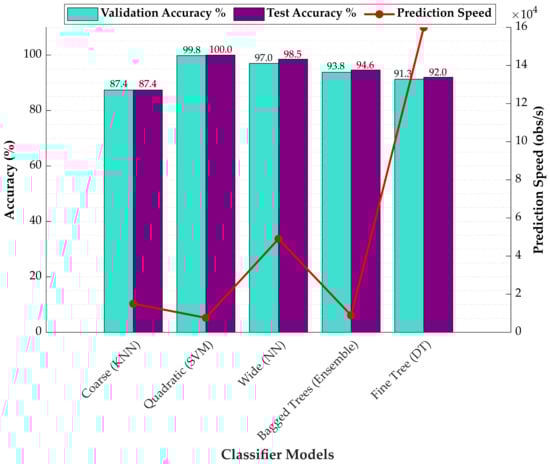
Figure 5. Comparison of the accuracy and prediction speed of the most successful type classifiers.

In this study, an additional analysis was conducted to determine the minimum thickness diversity that would maintain the model’s discriminative power, using the method that provided the highest accuracy in material type classification as a reference. To this end, the thickness levels in the dataset were gradually increased, and the change in classification performance was examined. In each scenario, the S₁₁ and S₂₁ scattering parameters corresponding to the relevant thickness values were used as features in the same manner. The findings presented in Table 12 indicate that the best-performing classifier maintains flawless accuracy even in scenarios where only three or more distinct thickness levels are evaluated together.

Table 12. Effect of different thickness values on classification performance.

Features	Validation Accuracy %	Test Accuracy %
${freq,S}_{11,1}^{\left(dB\right)},S_{21,1}^{\left(dB\right)}$	91.70	90.10
${freq,S}_{11,1}^{\left(dB\right)},S_{21,1}^{\left(dB\right)},S_{11,2}^{\left(dB\right)},S_{21,2}^{\left(dB\right)}$	99.30	99.30
${freq,S}_{11,1}^{\left(dB\right)},S_{21,1}^{\left(dB\right)},S_{11,2}^{\left(dB\right)},S_{21,2}^{\left(dB\right)},S_{11,3}^{\left(dB\right)},S_{21,3}^{\left(dB\right)}$	100	100
${freq,S}_{11,4}^{\left(dB\right)},S_{21,4}^{\left(dB\right)},S_{11,5}^{\left(dB\right)},S_{21,5}^{\left(dB\right)},S_{11,6}^{\left(dB\right)},S_{21,6}^{\left(dB\right)}$	100	100
${freq,S}_{11,7}^{\left(dB\right)},S_{21,7}^{\left(dB\right)},S_{11,8}^{\left(dB\right)},S_{21,8}^{\left(dB\right)},S_{11,9}^{\left(dB\right)},S_{21,9}^{\left(dB\right)}$	100	100
${freq,S}_{11,1}^{\left(dB\right)},S_{21,1}^{\left(dB\right)},S_{11,5}^{\left(dB\right)},S_{21,5}^{\left(dB\right)},S_{11,10}^{\left(dB\right)},S_{21,10}^{\left(dB\right)}$	100	100

The results reported in Table 12 were obtained by progressively increasing the number of thickness levels included in the feature set. In addition to consecutive thickness triplets (e.g., 1–2–3, 4–5–6, 7–8–9), a non-consecutive triplet (1–5–10) was also evaluated to assess sensitivity to the specific thickness selection. In all three-thickness scenarios, perfect classification accuracy was maintained.

Figure 6 presents the test confusion matrices of the best-performing classifiers for material type and thickness classification. As shown in Figure 6a, the Quadratic SVM (QSVM) achieved perfect class-wise discrimination for all material types. Similarly, Figure 6b demonstrates that the Fine KNN model provided near-perfect classification performance for material thickness, with no significant confusion observed between thickness levels. A confusion matrix summarizes the class-wise prediction performance by comparing true labels with the corresponding predicted labels, thereby providing insight into potential misclassification patterns.

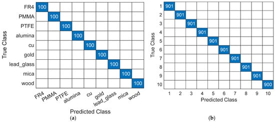
Figure 6. Test confusion matrices of the best-performing classifiers: (a) material type classification using Quadratic SVM; (b) material thickness classification using Fine KNN.

4. Conclusions and Discussion

In this study, the classification of material thickness and type was achieved by directly feeding the real, imaginary, and dB values derived from these components of the S₁₁ and S₂₁ scattering parameters into machine learning models. The objective of achieving high performance was to utilise the spectral resolution provided by the 1001 frequency point measurement range in the X band (8–12 GHz) and the 1–10 mm measurement range as the thickness value in the creation of the database. A comprehensive database was obtained through the utilisation of nine distinct materials, each exhibiting varying levels of conductivity. As a methodological approach, a comprehensive evaluation was conducted encompassing a wide range of models from diverse classifier families, five distinct training-testing split ratios, and 10-fold cross-validation. The elevated accuracy value obtained serves to demonstrate that microwave-based characterization is not confined to secondary calculations such as the estimation of dielectric constant, but rather that the S-parameter spectra themselves possess significant discriminative power. This feature serves to simplify the measurement-modelling workflow by eliminating conversion-induced error accumulation due to additional steps such as dielectric estimation. Consequently, it facilitates its integration into industrial applications. Moreover, favourable outcomes have been attained through the utilisation of conventional machine learning methodologies, which exhibit reduced computational expenses and more straightforward incorporation into real-time systems when contrasted with intricate deep learning-based approaches. In the context of an investigation into classification methodologies, the Fine KNN model, which attains 100% accuracy in thickness classification across the full range of data partitioning ratios, serves to illustrate that the amplitude and phase variations present in the S₁₁ and S₂₁ spectra are characterized by a regular, high-resolution structure that is directly proportional to thickness. This finding is consistent with the thickness-sensitive characteristic of material–wave interaction within the X-band measurement range. Conversely, the decline in performance of less sophisticated models, such as Linear Discriminant, decision trees, and naive Bayes, suggests that the spectral data possesses a degree of complexity necessitating non-linear decision boundaries. In material type classification, when it becomes difficult to distinguish materials exhibiting similar S-parameter profiles, including measurements of the same material at different thicknesses in the model, increased spectral diversity is ensured, and decision boundaries are formed more distinctly. The finding that the Quadratic SVM attained 100% accuracy in type classification suggests the presence of a robust and consistent spectral separation between the materials. It is noteworthy that the high performance is maintained even when only three different thickness levels are used, which demonstrates that material-specific spectral signatures can be distinguished independently of thickness variations. This has the significant advantage of simplifying system design by obviating the need to measure a wide thickness range in practical applications. In this respect, this study makes a significant contribution to the reduction in measurement costs and data collection burdens for microwave-based material recognition systems. Whilst the 100% accuracy values obtained in the study are impressive, it is important to assess the risk of overfitting in high-dimensional feature space due to the collection of data from 1001 frequency points for each sample. In this context, the performance of the model was systematically examined not only based on a single training–test split but also across five different training-test ratios (90/10, 80/20, 70/30, 60/40, and 50/50) and 10-fold cross-validation. The findings reveal that the models do not merely execute rote classification, but instead demonstrate the capacity to generalise material-specific spectral patterns. The response of model performance to data splitting ratios also yielded important methodological results. While the 90/10 ratio was found to provide stable performance for all algorithms in thickness classification, the optimal ratio in type classification was found to vary depending on the model type. This finding suggests that thickness information is more deterministic in nature, whereas material type information necessitates greater sample diversity. Distance-based classifiers such as KNN excelled in thickness classification due to the locally well-separated spectral patterns, whereas kernel-based SVM models provided superior discrimination in material type classification by capturing non-linear separations in high-dimensional feature space. Moreover, the joint analysis of prediction speed and training time metrics demonstrates that models such as Fine Tree and Linear Discriminant offer high speed advantages but have limited accuracy levels when compared to complex methods. Consequently, a performance-computational cost balance can be established depending on the application.

In the extant literature, the number of studies utilising scattering parameters measured in the microwave region in conjunction with machine learning is limited. The majority of existing studies present approaches that are focused on narrow-scope datasets, a small number of material types, or a single problem. This phenomenon is clearly illustrated in Table 13. In their study, Hien and Hong [13] proposed a thickness classification methodology that utilised dielectric constants derived exclusively from S-parameters. Harrsion et al. [14] concentrated on distinguishing a limited number of material types using a microwave sensor array. In contrast, Satriya et al. [15] sought to develop a wholly simulation-based approach for thickness estimation of biological tissue layers. A direct comparison between the studies is precluded by the significant disparities in data types, materials utilised, and the range of issues addressed. Consequently, a direct comparison in the literature in terms of material diversity, thickness range, data resolution, and methodological scope is not possible. Furthermore, the majority of extant research has focused exclusively on either material thickness or material type, and there is no comprehensive study that addresses both tasks together under the same data collection protocol. In this respect, the proposed study addresses this gap in the existing literature by providing an experimentally grounded benchmark for microwave-based non-destructive material characterization.

Table 13. Comparative summary of previous studies and the proposed method.

Study	Data/Method	Purpose	Model	Key Outcomes	Key Distinction/ Advancement of Current Study
Hien & Hong [13]	Dielectric constant derived from S-parameters	Thickness Classification 7–10.5 mm (8 Classes)	Deep neural network, support vector machine	Avg. Accuracy SVM—99.6% DNN—99.94%	Uses dielectric constant estimation requires intermediate computation; limited thickness range (7–10.5 mm)
Harrsion et al. [14]	Microwave Sensor Array	Material type classification (wood, cardboard, plastics)	Decision tree-based support vector machine (DSVM)	Avg. Accuracy 83.28%	Limited material diversity; does not address thickness classification
Satriya et al. [15]	HFSS-simulated S11 data	Tissue-layer thickness estimation (SAT, MT, VT)	Polynomial regression (RiPR/PR) models	RMSE SAT: 0.35 mm MT: 1.57 mm VT: 1.7 mm	Simulation-based; no material variety; no classification task
Proposed	Experimental (VNA-based) S-parameters	Material thickness and type classification (9 real-world materials) (1–10 mm)	Fine KNN, Quadratic SVM	Accuracy Thickness: Fine KNN-100% Type: QSVM-100%	Direct use of S11–S21 spectra without dielectric inversion; wide material diversity; dual-task evaluation; high-resolution 1001-point dataset; demonstrates that even 3 thickness levels ensure perfect material discrimination

This is achieved through the use of a wide variety of materials and by feeding the directly measured S-parameters into machine learning models.

In conclusion, this study has demonstrated that a machine learning-based approach utilising S-parameters directly offers high accuracy and reliable performance within the investigated thickness and material classification tasks. Although the proposed approach achieved very high classification accuracy, the reported findings are valid under the specific experimental conditions of this study, including the employed vector network analyzer, waveguide configuration, frequency range (8–12 GHz), and material thickness intervals. The feature construction strategy for material type classification was designed to reflect material-specific spectral characteristics across different thickness levels. Therefore, the generalizability of the results to different measurement devices, waveguide bands, or environmental conditions should be further investigated. Future studies will focus on validating the proposed methodology using different measurement setups and environmental settings to further strengthen the robustness and practical applicability of the approach. The findings indicate that in microwave-based NDT applications, the measurement pipeline can be simplified, the data collection range can be narrowed, and models suitable for real-time classification systems can be selected. While computational speed is an important indicator of real-time feasibility, practical deployment also depends on robustness to measurement noise and hardware constraints. In this study, the models were trained and evaluated using measurements acquired under controlled laboratory conditions, which likely reduced the impact of noise and external perturbations. As a result, the reported prediction speeds primarily reflect algorithmic efficiency rather than end-to-end system performance. From an implementation perspective, the relatively low computational complexity of the best-performing models, such as KNN and SVM variants, suggests that they could be deployed on embedded or edge platforms, provided that data acquisition and feature construction are appropriately optimized. However, systematic evaluation under noisy conditions and resource-constrained hardware remains an important direction for future work. Subsequent research could involve the development of a device design by optimising the frequency weighting across a broader range of materials, under different waveguide bands, and under varying temperature or environmental conditions.

References

- Liu, C.H.; Lacidogna, G. A Non-Destructive Method for Predicting Critical Load, Critical Thickness and Service Life for Corroded Spherical Shells under Uniform External Pressure Based on NDT Data. Appl. Sci. 2023, 13, 4172. [Google Scholar] [CrossRef]
- Mohamed Omar, M.F.; Abdul Rahim, S.K.; Ain, M.F.; Manaf, A.A.; Zainal Abidin, I.S.; Shamsan, Z.A. Antenna Performances Based on Distinctive Thickness-Dependent of Flexible Substrates: A Comprehensive Review. Ain Shams Eng. J. 2025, 16, 103417. [Google Scholar] [CrossRef]
- Jatulis, M.; Elghandour, E.; Elzayady, N. Evaluation of the Mechanical Properties of Aircraft Composite Materials after Indentation. J. Mech. Sci. Technol. 2023, 37, 5813–5821. [Google Scholar] [CrossRef]
- Kim, S.-H.; Lee, S.-Y.; Zhang, Y.; Park, S.-J.; Gu, J. Carbon-Based Radar Absorbing Materials toward Stealth Technologies. Adv. Sci. 2023, 10, e2303104. [Google Scholar] [CrossRef] [PubMed]
- Jiang, X.; Xu, Y.; Hu, H. Thickness Characterization of Steel Plate Coating Materials with Terahertz Time-Domain Reflection Spectroscopy Based on BP Neural Network. Sensors 2024, 24, 4992. [Google Scholar] [CrossRef] [PubMed]
- Ghattas, A.; Al-Sharawi, R.; Zakaria, A.; Qaddoumi, N. Detecting Defects in Materials Using Nondestructive Microwave Testing Techniques: A Comprehensive Review. Appl. Sci. 2025, 15, 3274. [Google Scholar] [CrossRef]
- Inês Silva, M.; Malitckii, E.; Santos, T.G.; Vilaça, P. Review of Conventional and Advanced Non-Destructive Testing Techniques for Detection and Characterization of Small-Scale Defects. Prog. Mater. Sci. 2023, 138, 101155. [Google Scholar] [CrossRef]
- Liu, C.; Liao, C.; Peng, Y.; Zhang, W.; Wu, B.; Yang, P. Microwave Sensors and Their Applications in Permittivity Measurement. Sensors 2024, 24, 7696. [Google Scholar] [CrossRef] [PubMed]
- Libby, H.L. Introduction to Electromagnetic Nondestructive Test Methods, 99th ed.; John Wiley & Sons: Nashville, TN, USA, 1971; ISBN 9780471534105. [Google Scholar]
- Blitz, J. Electrical and Magnetic Methods of Non-Destructive Testing, 2nd ed.; Chapman and Hall: London, UK, 1997; ISBN 9780412791505. [Google Scholar]
- Udpa, S.S.; Moore, P.O. Nondestructive Testing Handbook: Electromagnetic Testing; American Society for Nondestructive Testing (ASNT): Columbus, OH, USA, 2004; ISBN 9781571172853. [Google Scholar]
- Anker, A.S.; Butler, K.T.; Selvan, R.; Jensen, K.M.Ø. Machine Learning for Analysis of Experimental Scattering and Spectroscopy Data in Materials Chemistry. Chem. Sci. 2023, 14, 14003–14019. [Google Scholar] [CrossRef]
- Hien, P.T.; Hong, I.-P. Material Thickness Classification Using Scattering Parameters, Dielectric Constants, and Machine Learning. Appl. Sci. 2021, 11, 10682. [Google Scholar] [CrossRef]
- Harrsion, L.; Ravan, M.; Tandel, D.; Zhang, K.; Patel, T.; Amineh, R.K. Material Identification Using a Microwave Sensor Array and Machine Learning. Electronics 2020, 9, 288. [Google Scholar] [CrossRef]
- Satriya, A.B.; Tan, M.J.T.; Yoon, Y.-K. Machine Learning-Based Thickness Estimation of Abdominal Fat and Muscle Using Simulated Radio Frequency Scattering Parameters. In Proceedings of the 2024 21st International Conference on Electrical Engineering, Computing Science and Automatic Control (CCE), Mexico City, Mexico, 23–25 October 2024; pp. 1–6. [Google Scholar]
- Hinderhofer, A.; Greco, A.; Starostin, V.; Munteanu, V.; Pithan, L.; Gerlach, A.; Schreiber, F. Machine Learning for Scattering Data: Strategies, Perspectives and Applications to Surface Scattering. J. Appl. Crystallogr. 2023, 56, 3–11. [Google Scholar] [CrossRef]
- Yildirim, B.; Doutch, J.; Cole, J. Multi-Task Scattering-Model Classification and Parameter Regression of Nanostructures from Small-Angle Scattering Data. Digit. Discov. 2024, 3, 694–704. [Google Scholar] [CrossRef]
- Morales-Garcia, J.; Ramos-Sorroche, E.; Balderas-Diaz, S.; Guerrero-Contreras, G.; Munoz, A.; Santa, J.; Terroso-Saenz, F. Reducing Pollution Health Impact with Air Quality Prediction Assisted by Mobility Data. IEEE J. Biomed. Health Inform. 2025, 29, 9210–9220. [Google Scholar] [CrossRef] [PubMed]
- Muñoz, A.; Martínez-España, R.; Guerrero-Contreras, G.; Balderas-Díaz, S.; Arcas-Túnez, F.; Bueno-Crespo, A. A Multi-DL Fuzzy Approach to Image Recognition for a Real-Time Traffic Alert System. J. Ambient Intell. Smart Environ. 2025, 17, 101–116. [Google Scholar] [CrossRef]
- Li, J.; Zheng, K.; Gao, L.; Han, Z.; Li, Z.; Chanussot, J. Enhanced Deep Image Prior for Unsupervised Hyperspectral Image Super-Resolution. IEEE Trans. Geosci. Remote Sens. 2025, 63, 5504218. [Google Scholar] [CrossRef]
- Baker-Jarvis, J.; Janezic, M.D.; Domich, P.D.; Geyer, R.G. Analysis of Errors in the Permittivity Determination Using the Nicolson–Ross–Weir Method. NIST Technical Note 1355-R; National Institute of Standards and Technology: Boulder, CO, USA, 1993.
- Hong, J.-S.; Lancaster, M.J. Microstrip Filters for RF/Microwave Applicatiıons; John Wiley & Sons, Inc.: New York, NY, USA, 2001. [Google Scholar]
- Cortes, C.; Vapnik, V. Support-Vector Networks. Mach. Learn. 1995, 20, 273–297. [Google Scholar] [CrossRef]
- Cover, T.; Hart, P. Nearest Neighbor Pattern Classification. IEEE Trans. Inf. Theory 1967, 13, 21–27. [Google Scholar] [CrossRef]
- Dietterich, T.G. Ensemble Methods in Machine Learning. In Multiple Classifier Systems; Springer: Berlin/Heidelberg, Germany, 2000; pp. 1–15. ISBN 9783540677048. [Google Scholar]
- Zhang, G.P. Neural Networks for Classification: A Survey. IEEE Trans. Syst. Man Cybern. C Appl. Rev. 2000, 30, 451–462. [Google Scholar] [CrossRef]
- Quinlan, J.R. Learning Decision Tree Classifiers. ACM Comput. Surv. 1996, 28, 71–72. [Google Scholar] [CrossRef]
- Murphy, K.P. Machine Learning: A Probabilistic Perspective; MIT Press: London, UK, 2012; ISBN 9780262304320. [Google Scholar]
- Qu, L.; Pei, Y. A Comprehensive Review on Discriminant Analysis for Addressing Challenges of Class-Level Limitations, Small Sample Size, and Robustness. Processes 2024, 12, 1382. [Google Scholar] [CrossRef]
Disclaimer/Publisher’s Note: The statements, opinions and data contained in all publications are solely those of the individual author(s) and contributor(s) and not of MDPI and/or the editor(s). MDPI and/or the editor(s) disclaim responsibility for any injury to people or property resulting from any ideas, methods, instructions or products referred to in the content. |
© 2025 by the authors. Licensee MDPI, Basel, Switzerland. This article is an open access article distributed under the terms and conditions of the Creative Commons Attribution (CC BY) license.