Abstract
The Synthetic Aperture Radar Interferometry (InSAR) technique enables researchers to generate Digital Elevation Models (DEMs) from SAR data, which researchers widely apply in multi-temporal analyses, including ground deformation monitoring, susceptibility mapping, and analysis of spatial changes in erosion basins. In this study, we generated two interferometric DEMs from Sentinel-1 (S1, VV polarization) and TerraSAR-X (TSX, HH polarization, ascending orbit) data, processed in SNAP, over a mountainous sector of the central Andes in Chile. We assessed the accuracy of the DEMs against two reference datasets: the SRTM DEM and a high-resolution LiDAR-derived DEM. We selected 150 randomly distributed points across different slope classes to compute statistical metrics, including RMSE and MedAE. Relative to the LiDAR DEM, both sensors yielded rMSE values of approximately 20 m, increasing to 23–24 m when compared with the SRTM DEM. The MedAE, a metric less sensitive to outliers, was 3.97 m for S1 and 3.26 m for TSX with respect to LiDAR, and 7.07 m for S1 and 7.49 m for TSX relative to SRTM. We observed a clear positive correlation between elevation error and terrain slope. In areas with slopes greater than 45°, the MedAE exceeded 14 m relative to the LiDAR DEM and reached ~15 m relative to the SRTM for both S1 and TSX.
Keywords:
digital elevation model (DEM); Sentinel-1 (S1); TerraSAR-X (TSX); InSAR; central Andes; rMSE; MedAE 1. Introduction
A Digital Elevation Model (DEM) is an ordered matrix that represents the spatial distribution of elevations over an arbitrary datum in each area [1,2]. This type of data is fundamental to characterizing the Earth’s surface as a primary source of topographic information. DEMs are widely used across diverse research areas, including resource management, natural hazard and risk assessment, engineering and infrastructure planning, aeronautical safety, forestry, topographic mapping, and soil science [3,4,5,6]. An alternative to obtaining DEMs is the Interferometric Synthetic Aperture Radar (InSAR) technique, in contrast to traditional methods such as aerial photogrammetry, global positioning systems, and laser altimetry [7,8,9]. InSAR enables the generation of digital elevation models with medium spatial resolution for multitemporal studies of geological hazards, such as monitoring land deformation due to mass-movement processes, susceptibility analysis, and glacier mass balance [10,11,12].
The Andes Mountain range is one of the major landforms in Chile, characterized by complex physiography and difficult access. Elevation analysis in this region can benefit from the InSAR technique for large-scale, periodic DEM generation at a lower cost than other techniques [13]. In this way, several studies have demonstrated the usefulness of DEMs across multiple fields. For example, refs. [14,15,16] employ them for hydraulic modeling, while works such as [17,18] use interferometric models to analyze landslides and rockfalls.
Despite these advances, the performance of InSAR-derived DEMs strongly depends on sensor characteristics and radar wavelength, particularly in steep and geodynamically active mountainous environments. In this sense, the joint use of Sentinel-1 (C-band) and TerraSAR-X (X-band) data provides a valuable opportunity to assess the influence of wavelength and sensor configuration on DEM generation. Thus, a systematic comparison of DEMs derived from both platforms can help identify their respective strengths and limitations for optimal selection in mountainous regions.
The literature has demonstrated the advantages of the InSAR technique for producing periodic DEMs at large scales and at lower economic cost than other DEM generators [18,19].
Several authors have advanced the development of DEM generation using InSAR [20]. In [21,22], the authors demonstrate that one can achieve a high-quality DEM by optimizing the baseline. They propose merging ascending and descending interferograms to achieve high coherence while avoiding foreshortening and scale issues. Other researchers suggest simulating the output DEM under specific orbital and topographic conditions and incorporating external DEMs into the creation process. Applying algorithms to adjust phase errors caused by atmospheric artifacts to improve vertical resolution [23,24,25,26]. In mountainous areas, we recommend considering the satellite’s trajectory, particularly the illumination angle, to ensure an optimal perpendicular baseline between interferometric pairs and high image coherence [21,27,28].
In this regard, the European Space Agency (ESA) has made SAR images from the Sentinel-1 (S1) satellite freely available since 2014, with a spatial resolution suitable for studying Earth’s surface (and generating DEMs). Moreover, the German Aerospace Center (DLR) and the space division of European Aeronautic Defence and Space (EADS Astrium) have provided TerraSAR-X (TSX) satellite images since 2007, designed for similar purposes at a high resolution. In this way, this study focuses on the quality of DEMs generated from both platforms in complex environments, such as the Andes Mountains.
Previously, various studies have been conducted in mountainous terrains, obtaining different results. For instance, refs. [3,29,30] report rMSE values of 8.7–320 m using S1 sensors, while refs. [28,31,32] document rMSE results of 6–13 m with TSX sensors. Based on this, the present study aims to evaluate DEMs derived from InSAR imagery from the S1 and TSX satellites, in comparison with two reference DEMs (LiDAR and SRTM) in a mountainous area of central Chile. For this, statistical metrics were used across different slope ranges, namely absolute, squared, and percentage error, variance explanation, and correlation.
We have organized this article as follows: after the introduction, context, and definition of objectives, we present the study area and the image collections used. Next, we describe the InSAR processing using SNAP software. In the results section, we first present the generation of the interferometric DEMs. Subsequently, we compare the DEM-S1 and DEM-TSX profiles with the reference DEMs, and finally, we present the results of the vertical accuracy assessment. The article concludes with a discussion and conclusion.
2. Materials and Methods
2.1. Study Area
The study area corresponds to a mountainous sector in central Chile, near the city of Santiago, located between 32°50′ and 33°26′ south latitude and between 69°58′ and 70°32′ west longitude, covering an area of approximately 1600 km2 (Figure 1). The region has a Mediterranean climate, characterized by an average annual precipitation of 341 mm, concentrated in the winter months, and a prolonged dry season lasting 7 to 8 months [33]. Elevation in the area ranges from 1000 to 6000 m above sea level, with an average elevation of 3190 m.
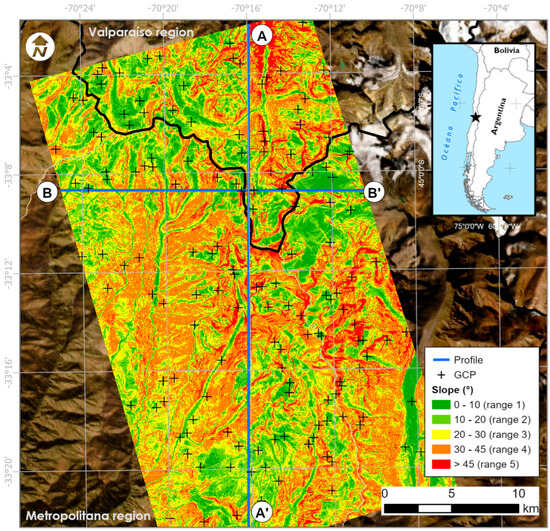
Figure 1.
Study area. Profile A–A’ runs north–south, and profile B–B’ runs east–west; we used both for comparisons between the interferometric DEM and the reference DEMs. The reclassification of slope ranges was carried out based on the criteria proposed by [34].
2.2. Data Acquisition
2.2.1. S1 and TSX Data
The interferometric pairs used in the evaluation correspond to SAR images from the S1 satellite, which orbits at 693 km and acquires data in C-band (5.405 GHz). These images have a Single Look Complex (SLC) processing level, cover 250 km, and have a 12-day repeat cycle. We downloaded them from the Alaska Satellite Facility’s free server [35]. Ascending and descending orbit images from S1 were combined, using two pairs from each orbit to cover the entire study area.
The TSX images, from the TerraSAR-X satellite orbiting at an altitude of 514 km, operate in the X-band (9.65 GHz), use SSC (Single Look Slant Range Complex) processing, cover 150–200 km, and have a temporal resolution of 11 days (Table 1). The incidence near-angle for S1 and TSX was 31° and 33.7°, respectively. The incidence of far-angle was 46 and 36.98 for S1 and TSX.

Table 1.
Characteristics of interferometric pairs. Where m is the master image, s is the slave image, Bp is the perpendicular baseline, and Bt is the temporal baseline.
Meteorological stations located in the study area recorded no rainfall during the image acquisition period [36].
2.2.2. Reference DEMs
We used two reference DEMs from the mountainous region of central Chile to evaluate the DEMs generated from S1 and TSX images. The first reference is a product generated by airborne LiDAR using a Trimble Harrier 68i system (2020). This has higher accuracy with a spatial resolution of 1 m. The second reference is provided by the Shuttle Radar Topography Mission (SRTM) from the year 2000, downloaded from the EarthExplorer platform [37]. This product is freely available with a resolution of 30 m.
We extracted 150 Ground Control Points (GCPs) from each reference DEM (LiDAR and SRTM) to assess the interferometric DEMs across different slope ranges.
2.3. Interferometric Processing of S1 and TSX
InSAR analyzes the phase-interference pattern of signals from two SAR images. A small antenna aboard an airborne or satellite platform transmits microwave signals sequentially along a flight path at an oblique angle. From these signals, the backscattered component is measured based on surface characteristics, including amplitude (echo response strength) and phase, which indicates the position of a point at a given moment in the wave cycle [27,38,39,40,41].
Interferometry uses the phase difference between two SAR observations acquired from slightly different sensor positions (master and slave). By combining these phases after co-registration, we can generate an interferogram, from which we extract topographic information and possible ground deformation.
The phase variation (δϕ) between acquisitions is the sum of the topographic phase (ϕ DEM), surface deformation (ϕ deform), atmospheric conditions such as humidity, temperature, and pressure changes (ϕ atm), and noise, which includes different viewing angles and volume scattering (ϕ noise) [27,42,43,44]. This is shown in Equation (1).
δϕ = ϕ (DEM) + ϕ (deform) + ϕ (atm) + ϕ (noise).
For the DEM generation, we assume that there is no ground deformation (considered zero), and that the contribution of noise phase (change of the scatterers, different look angle, and volume scattering) and atmospheric phase (humidity, temperature, and pressure changes between the two acquisitions) to the total phase difference is minimal [2,27]. Thus, this contribution can be neglected. Consequently, we consider the phase variation equal to the topographic phase, as shown in Equation (2).
δϕ = ϕ (DEM).
We processed S1 and TSX images following the methodological workflow described in Figure 2. We used the Sentinel Application Platform (SNAP) software 8.0, developed by the European Space Agency.
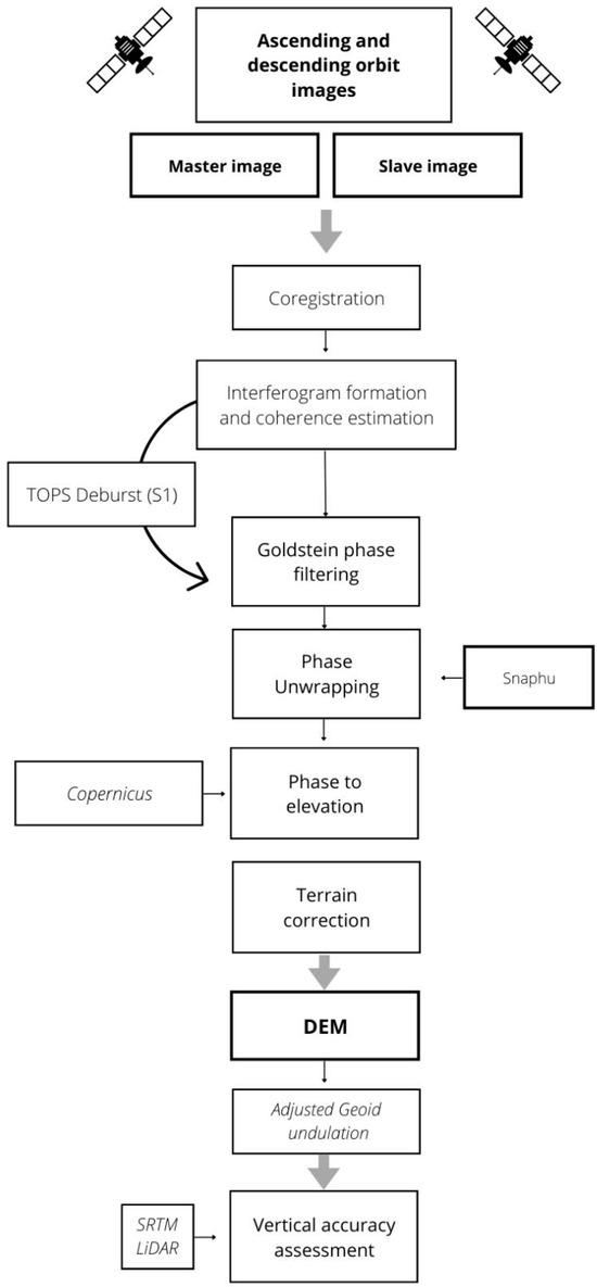
Figure 2.
Workflow for DEM generation from S1 and TSX images. Modified from Braun, 2021 [2].
First, we estimated the baseline from the orbital data. We generated the interferogram before co-registering the SAR images. For the S1 pair, the interferogram’s border fringes, resulting from the TopSAR or IW acquisition mode, were removed. For the TSX images acquired in StripMap mode, this step was not necessary.
Next, the Goldstein filter, which uses a Fast Fourier Transform (FFT), was applied to improve the image’s signal-to-noise ratio. This step is essential for phase unwrapping, which converts the phase from its original 2π cycle modulation to its absolute value. We performed this procedure using the SNAPHU algorithm (https://step.esa.int/main/snap-supported-plugins/snaphu/ (accessed on 21 December 2025)) [45], which operates as a plugin within the SNAP software.
Finally, in the SNAP Terrain Correction module, we geocoded the images to correct inherent SAR geometric distortions using the 30 m Copernicus Digital Elevation Model (DEM) provided by SNAP itself, thereby obtaining a product projected in a geographic coordinate system.
The DEMs obtained with the SNAP software contain ellipsoidal heights (h). To get models with orthometric heights (H) comparable to the reference models, it is necessary to apply a correction for geoid undulation (N) [14,46,47].
We obtained the N values at the Ground Control Points (GCPs) from (https://geographiclib.sourceforge.io/ (accessed on 5 January 2023)) using the EGM2008 geoid model, and the average geoid undulation in the study area is approximately 29.71 m. Finally, we subtracted this value from the generated DEMs using the formula H = h − N.
2.4. Vertical Accuracy Assessment
We generated a DEM average from the S1 images in ascending and descending orbits. Both the DEM-S1 and DEM-TSX were reprojected to the UTM coordinate system (Zone 19, southern hemisphere) and resampled to a 13-m resolution using the nearest-neighbor method. Subsequently, we created elevation profiles and a slope model to analyze the topographic variability of the study area. To extract height values from each DEM, a sample of 150 control points was randomly distributed across five slope ranges (30 points per range), as shown in Figure 1.
We evaluated the elevations (DEM) extracted from the control points using the LiDAR 2020 and SRTM 2000 reference DEMs. For this, standard error scores were used, such as the root Mean Squared Error (rMSE) [48], Mean Absolute Error (MAE) [48], Median Absolute Error (MedAE) [48], Mean Absolute Percentage Error (MAPE) [49], Explained Variance (EV) [49], and Pearson Correlation (Corr) [50], as shown in Equations (3)–(8), respectively. Additionally, the standard deviation was calculated. The MedAE and MAPE compute scores to detect errors in skew measurements.
In previous equations, Zni is the elevation value of point i in the generated DEM, Zri is the elevation value from the reference DEM of point i, n is the number of control points, variance () is the function that calculates the variance of the data, and mean () is the function that calculates the mean of the data.
3. Results
3.1. InSAR DEM Generation
The coherence values of the images (Figure 3), obtained during DEM generation, serve as a key indicator of the quality of the interferometric phase. In this study, the interferometric pair from the Sentinel-1 sensor, with VV polarization in ascending and descending orbits, showed a mean coherence of 0.56 and a standard deviation of 0.21, which represents a good result for a mountainous area. In contrast, the descending interferometric pair from the TerraSAR-X sensor in HH polarization showed a mean coherence of 0.24 and a standard deviation of 0.11, indicating low coherence in numerous pixels (Figure 3).
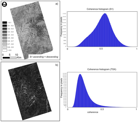
Figure 3.
(a) Coherence images from Sentinel-1 sensor (VV polarization), combining ascending and descending orbits, and corresponding coherence histogram. (b) Coherence images from the TerraSAR-X sensor (HH polarization) and associated coherence histogram. White areas indicate coherence values close to 1, while dark areas represent values close to 0.
Figure 4 shows the interferograms (range −π to π) corresponding to the S1 and TSX images. The TSX interferogram exhibits higher noise and lower coherence, attributed to temporal variations in backscattering mechanisms between acquisitions (temporal correlation). These variations are associated with a more extended temporal baseline (66 days) and, probably, the tropospheric delay between the two acquisitions due to changes in the local climate, and the signal penetration is different for each band, in which the C band (λ 5.6 cm) has greater penetration than the X band (λ 3.1 cm). Additionally, approximately 75% of the study area has slopes greater than 20°, and 38.78% are very steep, a typical characteristic of the central Chilean Andes. These complex topographic conditions can introduce geometric errors that significantly affect interferometric coherence.
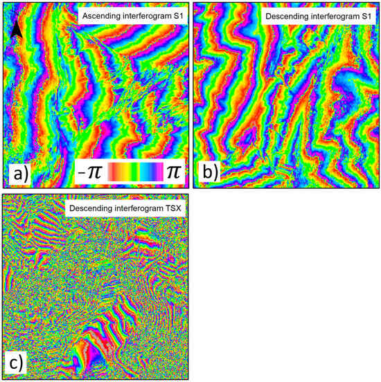
Figure 4.
(a) Ascending interferogram S1. (b) Descending interferogram S1. (c) Descending interferogram TerraSar-X.
Figure 5 displays the DEMs generated from InSAR, along with their corresponding hillshades. DEM-S1 presents elevation values ranging from 1356.63 to 5438.76 m, while the DEM-TSX ranges from 1357.26 to 5438.65 m. The differences between the minimum and maximum values of both models are in the millimeter range. For statistical evaluation against the reference DEMs, we resampled both models to 13 m. No apparent errors, such as data gaps or noticeable artifacts, were observed in the hillshades derived from the S1 and TSX DEMs.
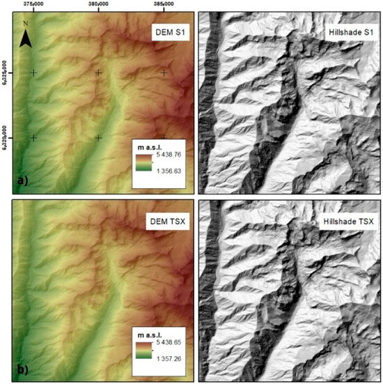
Figure 5.
(a) DEM InSAR and hillshade Sentinel-1, 2017. (b) DEM InSAR and hillshade TerraSar-X, 2017.
On the other hand, we found the most significant discrepancies between the DEM-S1 and the LiDAR DEM in areas affected by material removal activities, such as mining operations, where differences of up to 280 m occurred in the open-pit mine. Likewise, we identified underestimation of elevation in watershed-divided areas, with errors exceeding 100 m.
3.2. Comparison of DEM-S1 and DEM-TSX Profiles with SRTM and LiDAR Reference DEMs
In Figure 1, the traces of profiles A–A′ (N–S) and B–B′ (E–W), defined for the comparative evaluation of the generated DEMs, are shown. Figure 6 displays the resulting profiles extracted from the DEM-S1 and DEM-TSX models, superimposed on the SRTM reference DEM. These profiles reveal the altimetric variability of the InSAR models in relation to SRTM.
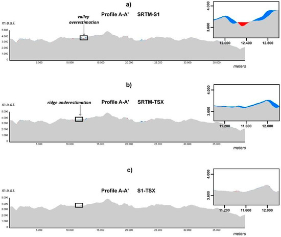
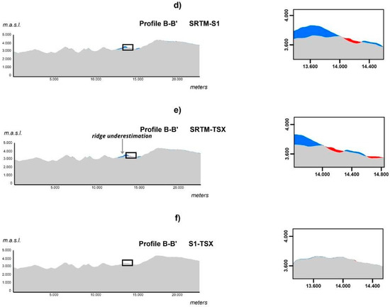
Figure 6.
Profiles A–A’ (NS) in the study area. (a) The comparison between DEM-S1 and SRTM. (b) The comparison between DEM-TSX and SRTM. (c) The comparison between DEM-S1 and DEM-TSX; next to this profile, a zoomed-in example is provided to illustrate the differences in greater detail. Blue areas indicate underestimations of the interferometric DEM values relative to the SRTM reference DEM, whereas red areas highlight overestimations of altitude values compared to the reference DEM. Profiles B–B’ (EW) in the study area. (d) The comparison between DEM-S1 and SRTM. (e) The comparison between DEM-TSX and SRTM. (f) The comparison between DEM-S1 and DEM-TSX; next to this profile, a zoomed-in example is included to provide greater detail of the observed differences. Blue areas indicate underestimations of the interferometric DEM values relative to the SRTM reference DEM, while red areas indicate sectors where altitude values are overestimated with respect to the reference DEM.
The blue areas indicate sectors where both DEM-S1 and DEM-TSX underestimate altitude compared to SRTM, while the red regions correspond to zones where both models overestimate it. In general, there is a tendency to overestimate altitude in flatter areas of the study zone, particularly in valleys. In addition, these products tend to underestimate the values in mountainous regions, where steep slopes predominate.
The comparison profiles of the S1 and TSX sensors show similar elevation values, as observed in Figure 6c,f.
In Figure 7, profiles A–A′ (N–S) and B–B′ (E–W) are shown for the DEMs derived from S1 and TSX images, including the LiDAR reference DEM. Profile B–B′ shows an overestimation of elevation values in the areas corresponding to the open-pit mines of Los Bronces (Anglo American) and Andina (Codelco), likely due to the continuous removal and accumulation of material in these extraction zones.
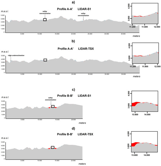
Figure 7.
Profile A–A’ (NS) y B–B’ (WE) in the study area. Profiles (a,c) show the comparison between DEM-S1 and LiDAR. Profiles (b,d) show the comparison between DEM-TSX and LiDAR.
It is important to note that we generated the interferometric DEMs for 2017; in contrast, the LiDAR reference DEM corresponds to 2020. This suggests significant topographic changes during this period due to mining operations.
The differences between the S1 and TSX DEMs relative to SRTM indicate that steep hillsides, glaciers, and areas altered by mining activities (Figure 8) exhibit the largest elevation differences.
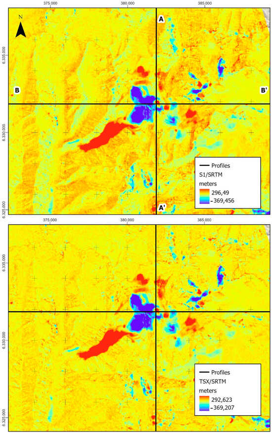
Figure 8.
Profile A–A’ (NS) y B–B’ (WE) in the study area. (top) The difference between S1 DEM and SRTM. (bottom) The difference between TSX DEM and SRTM.
3.3. Vertical Accuracy Assessment
In this section, we describe the assessment of elevation values generated from S1 (DEM-S1) and TSX (DEM-TSX), compared with two reference values extracted from SRTM and LiDAR, respectively.
First, in Figure 9, we depict the distribution of DEM values across the different sources. We do not observe any significant differences or groups of outliers across all configurations. Moreover, there is a tendency toward a normal distribution, with several values close to the mean and an exponential dispersion around it.
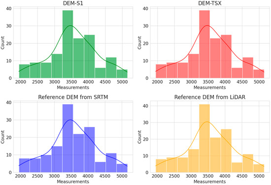
Figure 9.
Overview of the distribution of DEM values across different data sources.
In addition, we show the overall error scores in Table 2. Here, we observe that when SRTM is used as the reference DEM, the DEM-S1 values fit the elevation better, with lower error, higher explained variance, and higher correlation than DEM-TSX. However, when LiDAR serves as the reference DEM, DEM-TSX values fit better than those from DEM-S1. Nevertheless, with both DEMs, DEM-S1 and DEM-TSX, the correlation to the reference DEM exceeds 99%. In addition, these DEMs explain more than 99% of the variance in the reference DEMs.
Table 2.
Metric scores between different DEM sources and references from SRTM and LiDAR.
Furthermore, we show the MedAE and MAPE scores at different slope ranges in Figure 10, increasing from 1 to 5. We observe a slight tendency for errors in the MedAE and MAPE scores to increase as the slope range increases. This becomes clearer in the MedAE score when LiDAR serves as the reference DEM. This suggests that at higher slope ranges, estimating the DEM from either S1 or TSX sources becomes more difficult.
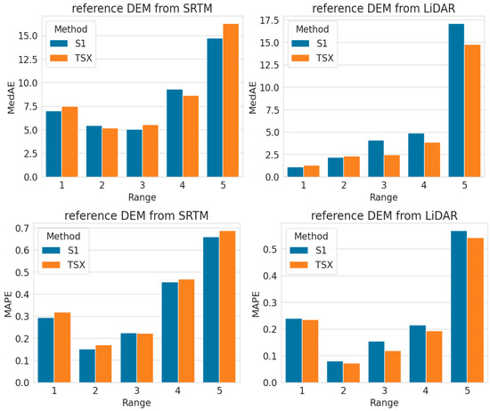
Figure 10.
MedAE and MAPE scores at different slope ranges for S1-based and TSX-based DEM compared to either SRTM (first column) or LiDAR (second column) as the reference DEM.
Meaning that the DEM measurements from LiDAR are more complex to estimate compared to the ones from SRTM at higher slope ranges. Nevertheless, at lower slope ranges, DEM measurements based on SRTM are more difficult to estimate than those from LIDAR.
The DEMs generated using the InSAR technique show high elevation similarity between the two sensors. Regarding the statistical metrics used, the overall Root Mean Squared Error (RMSE) relative to the LiDAR reference DEM was approximately 20 m for both S1 and TSX. When compared with the SRTM DEM, the RMSE values were 23 m for S1 and 24 m for TSX.
Using the Median Absolute Error (MedAE), a metric robust to outliers, the results against the LiDAR DEM were close to 4 m for S1 and 3 m for TSX. Compared with the SRTM DEM, the MedAE was approximately 7 m for both sensors.
Regarding terrain slope, we observed that elevation differences increase in proportion to the degree of inclination. In areas with slopes greater than 45°, MedAE values exceeded 14 m for both sensors relative to the LiDAR DEM, reaching approximately 15 m relative to the SRTM DEM. In contrast, in the first two slope ranges, MedAE values against the LiDAR DEM were below 2.5 m for both S1 and TSX, whereas in those same ranges, errors compared to the SRTM DEM exceeded 5 m.
4. Discussion
According to [21,27], an optimal interferometric pair for DEM generation should have a perpendicular baseline (Bp) of 150–300 m. When Bp is less than 30 m, sensitivity to phase noise increases, whereas values above 450 m tend to reduce coherence and, therefore, the quality of the interferogram [44,51]. In this study, the S1 interferometric pairs showed Bp values between 24 and 100 m, since this sensor is optimized for DInSAR studies [2] rather than precise DEM generation. In contrast, the TSX pair showed a Bp of 184 m, which is more suitable for this type of analysis.
In the mountainous central Andes of Chile, geomorphological conditions, with ridges aligned parallel to the satellite orbits, generate shadow zones and foreshortening that degrade interferometric coherence. This is stronger on slopes facing away from the sensor. We noticed this based on high rMSE values in steep areas due to low coherence. On the other hand, the low coherence of TSX images is probably due to the C band having greater penetration than the X band [2,27,52]. However, applying calibration and combining ascending and descending orbits in S1 enabled coherence values above 0.5, a threshold considered indicative of good quality for the interferometric phase [24]. Although the coherence of the TSX pair was lower (0.24), the rMSE values obtained were comparable to those of Sentinel-1.
Although the standard SNAP workflow applies the Goldstein phase filter for noise reduction, it is essential to acknowledge that more advanced phase-filtering and coherence-enhancement techniques could further improve DEM accuracy. Particularly in areas characterized by low coherence and strong phase variability. Non-local filtering approaches [53], block-matching methods [54], and more recent multilevel or learning-based algorithms have shown promising results in preserving phase information in complex terrains. The systematic implementation and evaluation of these techniques were beyond the scope of this study but represent a relevant direction for future research.
The elevation profiles in this study exhibited patterns similar to those described in previous studies [2,55]. This corresponds to an overestimation of altitude in flat areas (valleys) and an underestimation in mountainous regions with steep slopes. The A–A′ and B–B′ profiles obtained in this study are consistent with this behavior (Figure 6).
Statistical metrics confirmed that using the Median Absolute Error (MedAE) reduces the influence of outliers, improving evaluation accuracy. Compared to similar studies in the Andean region [29,30,46,47], favorable results were obtained. Concretely, for the interferometric model derived from TSX, despite its low coherence. The MedAE was similar to that reported in other studies conducted in high-mountain areas [29,31,32,46].
RMS values reported for DEMs generated from Sentinel-1 imagery in mountainous terrain reach 321 m [29] and between 39 and 58 [30]; TerraSAR-X data show an RMSE of 5.52 m [31]; TanDEM-X products exhibit RMSE values ranging between 11.99 and 13.01 m [32]; and PAZ-derived DEMs in similar environments range from 21 to 27 m [46]. In this study, when comparing the DEMs generated from S1 and TSX with the SRTM reference model, the resulting RMSE values were 23.26 m and 24.05 m, respectively. Moreover, as noted by [30], slopes greater than 35° will lead to larger errors in DEM generation, consistent with the findings of this study.
We recommend using images from the TanDEM-X mission (part of the same constellation) to improve coherence in TSX interferometric pairs, as it is explicitly designed for DEM generation and operates in tandem with TSX, reducing the temporal interval between acquisitions.
A relevant technical aspect was the need to convert ellipsoidal elevation data to orthometric heights, since SNAP generates values referenced to the ellipsoid. This adjustment was essential to ensure a valid comparison with the reference DEMs.
In line with [56], DEMs generated from InSAR data exhibit inherent errors, arising from acquisition geometry and processing, and can be affected by terrain morphology and land use. In this case, the steep slopes of the Andes significantly influence the accuracy obtained.
Furthermore, there are clear uncertainty considerations beyond our pixel-wise assessment. While the present study relies on point-based validation and therefore cannot derive spatially continuous uncertainty maps, we discuss the expected spatial distribution of elevation errors based on InSAR imaging geometry and terrain characteristics. In mountainous regions, elevation errors are expected to exhibit systematic spatial patterns driven by local slope, aspect, and sensor incidence angle. Steeper slopes oriented toward the radar line of sight may experience increased sensitivity to geolocation errors and residual layover effects, whereas slopes facing away from the sensor are more prone to shadowing and reduced coherence, potentially degrading elevation retrieval accuracy. Variations in local incidence angle can further modulate these effects, influencing the strength and stability of the backscattered signal and, consequently, the reliability of interferometric or pixel-based height estimates.
In this context, the slope-dependent analysis presented in this study can be interpreted as a partial proxy for spatially varying uncertainty, as slope encapsulates several geometric conditions that govern InSAR measurement performance. However, we emphasize that these considerations remain conceptual and cannot be quantified explicitly using the available point observations. A comprehensive spatial uncertainty characterization would require spatially continuous reference data and dedicated analysis of acquisition geometry, coherence, and terrain orientation, which lies beyond the scope of the present work.
5. Conclusions
This study demonstrates the potential of using multitemporal SAR data for DEM generation in complex mountainous environments with Sentinel-1 and TerraSAR-X data. The combination of ascending and descending orbits, together with processing in SNAP software, enabled the generation of DEMs with sufficient accuracy for environmental, land management, and hydrological basin analyses.
The DEMs generated using the InSAR technique with Sentinel-1 and TerraSAR-X show similar elevation values and comparable metrics against reference models, especially when using robust indicators such as the MedAE. Although the Sentinel-1 pairs have a perpendicular baseline shorter than optimal for DEM generation, the combination of ascending and descending orbits enabled coherence values above 0.5, sufficient to obtain acceptable results in mountainous areas.
The most significant elevation differences were observed in areas with steep slopes and in zones affected by mining activity, where the interferometric models significantly under- or overestimated topography relative to the LiDAR reference DEM. It has been confirmed that MedAE is a more appropriate metric than rMSE for accuracy assessment in this type of study, due to its lower sensitivity to outliers.
The multitemporal approach, based on interferometric pairs acquired at different dates, represents a viable and cost-effective alternative for updating topographic models in areas where high-resolution data are limited (e.g., ALOS, SRTM, and other global-scale DEMs). Furthermore, it demonstrates the usefulness of comparing DEMs obtained in different years with recent reference models, like LiDAR, to detect topographic changes associated with natural phenomena or anthropogenic activities, such as mining.
Author Contributions
Conceptualization, F.F., P.V.-P., P.O. and W.P.-M.; methodology, F.F. and F.M.; software, F.F. and F.M., formal analysis, F.F., P.V.-P. and F.M.; investigation, F.F. and P.V.-P.; resources, P.V.-P. and W.P.-M.; data curation, F.F., F.M. and P.V.-P.; writing—original draft preparation, P.V.-P. and F.F.; writing—review and editing, P.V.-P., F.F., F.M., W.P.-M. and P.O.; visualization, P.V.-P. and F.M. All authors have read and agreed to the published version of the manuscript.
Funding
This research was supported by internal funding from Universidad Mayor through the Publication Development Fund (FDP), 2021–2022 call (grant PEP I-2022004).
Data Availability Statement
The Sentinel-1 dataset is available from https://dataspace.copernicus.eu/, which is an open ecosystem that provides free and instant access to a wide range of Copernicus Sentinel data and services. On the other hand, the TSX data is subject to restrictions.
Acknowledgments
The authors thank the Magíster en Teledetección, Universidad Mayor, Chile.
Conflicts of Interest
The authors declare no conflicts of interest.
Correction Statement
This article has been republished with a minor correction to the readability of Figure 1. This change does not affect the scientific content of the article.
References
- Moore, I.D.; Grayson, R.B.; Ladson, A.R. Digital terrain modelling: A review of hydrological, geomorphological, and biological applications. Hydrol. Process. 1991, 5, 3–30. [Google Scholar] [CrossRef]
- Braun, A. Retrieval of digital elevation models from Sentinel-1 radar data–open applications, techniques, and limitations. Open Geosci. 2021, 13, 532–569. [Google Scholar] [CrossRef]
- Makineci, H.B.; Karabörk, H. Evaluation digital elevation model generated by synthetic aperture radar data. ISPRS Arch. Photogramm. Remote Sens. Spat. Inf. Sci. 2016, XLI–B1, 57–62. [Google Scholar] [CrossRef]
- Gheorghe, M.; Voda, A.-I. InSAR digital terrain models for mining areas based on Sentinel-1 imagery: A case study in Căliman area. Geopatterns 2020, 5, 21–26. [Google Scholar] [CrossRef]
- Głowacki, T.; Kasza, D. Assessment of morphology changes of the end moraine of the Werenskiold Glacier (SW Spitsbergen) using active and passive remote sensing techniques. Remote Sens. 2021, 13, 2134. [Google Scholar] [CrossRef]
- Kakavas, M.P.; Nikolakopoulos, K.G. Digital Elevation Models of Rockfalls and Landslides: A Review and Meta-Analysis. Geosciences 2021, 11, 256. [Google Scholar] [CrossRef]
- Zhou, H.; Zhang, J.; Gong, L.; Shang, X. Comparison and validation of different DEM data derived from InSAR. Procedia Environ. Sci. 2012, 12, 590–597. [Google Scholar] [CrossRef][Green Version]
- Deilami, K.; Hashim, M. Very High Resolution Optical Satellites for DEM Generation: A Review. Eur. J. Sci. Res. 2011, 49, 542–554. [Google Scholar]
- Bhushan, S.; Shean, D.; Alexandrov, O.; Henderson, S. Automated Digital Elevation Model (DEM) Generation from Very-High-Resolution Planet SkySat Triplet Stereo and Video Imagery. ISPRS J. Photogramm. Remote Sens. 2021, 173, 151–165. [Google Scholar] [CrossRef]
- Azmoon, B.; Biniyaz, A.; Liu, Z. Use of High-Resolution Multi-Temporal DEM Data for Landslide Detection. Geosciences 2022, 12, 378. [Google Scholar] [CrossRef]
- Li, J.; Wang, W.; Han, Z.; Li, Y.; Chen, G. Exploring the Impact of Multitemporal DEM Data on the Susceptibility Mapping of Landslides. Appl. Sci. 2020, 10, 2518. [Google Scholar] [CrossRef]
- Yan, L.; Wang, J.; Shao, D. Glacier Mass Balance in the Manas River Using Ascending and Descending Pass of Sentinel 1A/1B Data and SRTM DEM. Remote Sens. 2022, 14, 1506. [Google Scholar] [CrossRef]
- Geymen, A. Digital elevation model (DEM) generation using the SAR interferometry technique. Arab. J. Geosci. 2014, 7, 827–837. [Google Scholar] [CrossRef]
- Burgos, V.H.; Salcedo, A.P. Modelos Digitales de Elevación: Tendencias, Correcciones Hidrológicas y Nuevas Fuentes de Información; Encuentro de Investigadores en Formación en Recursos Hídricos: Ezeiza, Buenos Aires, Argentina, 2014. Available online: http://www.ina.gov.ar/ifrh-2014/Eje1/1.11.pdf (accessed on 1 October 2015).
- Md Ali, A.; Solomatine, D.P.; Di Baldassarre, G. Assessing the Impact of Different Sources of Topographic Data on 1-D Hydraulic Modelling of Floods. Hydrol. Earth Syst. Sci. 2015, 19, 631–643. [Google Scholar] [CrossRef]
- Mohammadi, A.; Karimzadeh, S.; Jalal, S.J.; Kamran, K.V.; Shahabi, H.; Homayouni, S.; Al-Ansari, N. A Multi-Sensor Comparative Analysis on the Suitability of Generated DEM from Sentinel-1 SAR Interferometry Using Statistical and Hydrological Models. Sensors 2020, 20, 7214. [Google Scholar] [CrossRef]
- Dai, K.; Li, Z.; Tomás, R.; Liu, G.; Yu, B.; Wang, X.; Singleton, A.; Milledge, D.; Jordan, C.; Stockamp, J. Monitoring Activity at the Daguangbao Mega-Landslide (China) Using Sentinel-1 TOPS Time Series Interferometry. Remote Sens. Environ. 2016, 186, 501–513. [Google Scholar] [CrossRef]
- Casagli, N.; Cigna, F.; Bianchini, S.; Hölbling, D.; Füreder, P.; Righini, G.; Gigli, G.; Tofani, V.; D’Amato Avanzi, G.; Lanteri, L.; et al. Landslide Mapping and Monitoring by Using Radar and Optical Remote Sensing: Examples from the EC-FP7 Project SAFER. Remote Sens. Appl. Soc. Environ. 2016, 4, 92–108. [Google Scholar] [CrossRef]
- Cigna, F.; Bianchini, S.; Righini, G.; Proietti, C.; Casagli, N. Updating Landslide Inventory Maps in Mountain Areas by Means of Persistent Scatterer Interferometry (PSI) and Photo-Interpretation: Central Calabria (Italy) Case Study. In Proceedings of the International Conference Mountain Risks, Florence, Italy, 24–26 November 2010. [Google Scholar]
- Massonnet, D.; Rabaute, T. Radar interferometry: Limits and potential. IEEE Trans. Geosci. Remote Sens. 1993, 31, 455–464. [Google Scholar] [CrossRef]
- Crosetto, M.; Crippa, B. Quality assessment of interferometric SAR DEMs. Int. Arch. Photogramm. Remote Sens. 2000, 33, 46–53. [Google Scholar]
- Yamane, N.; Fujita, K.; Nonaka, T.; Shibayama, T.; Takagishi, S. Accuracy Evaluation of DEM Derived by TerraSAR-X Data in the Himalayan Region. Int. Arch. Photogramm. Remote Sens. Spatial Inf. Sci. 2008, 37, 203–208. [Google Scholar]
- Abdelfattah, R.; Nicolas, J.M. Topographic SAR interferometry formulation for high-precision DEM generation. IEEE Trans. Geosci. Remote Sens. 2002, 40, 2415–2426. [Google Scholar] [CrossRef]
- Zhou, C.; Ge, L.; E, D.; Chang, H. A case study of using external DEM in InSAR DEM generation. Geo-Spat. Inf. Sci. 2005, 8, 14–18. [Google Scholar] [CrossRef]
- Liao, M.; Wang, T.; Lu, L.; Zhou, W.; Li, D. Reconstruction of DEMs from ERS-1/2 tandem data in mountainous area facilitated by SRTM data. IEEE Trans. Geosci. Remote Sens. 2007, 45, 2325–2335. [Google Scholar] [CrossRef]
- Liu, Z.; Zhou, C.; Fu, H.; Zhu, J.; Zuo, T. A framework for correcting ionospheric artifacts and atmospheric effects to generate high accuracy InSAR DEM. Remote Sens. 2020, 12, 318. [Google Scholar] [CrossRef]
- Ferretti, A.; Monti-Guarnieri, A.; Prati, C.; Rocca, F.; Massonnet, D. InSAR Principles—Guidelines for SAR Interferometry Processing and Interpretation, TM-19; ESA Publications: Noordwijk, The Netherlands, 2007; Available online: http://hdl.handle.net/11311/550055 (accessed on 23 March 2022).
- Wang, X.; Liu, L.; Shi, X.; Huang, X.; Geng, W. A High Precision DEM Extraction Method Based on InSAR Data. ISPRS Ann. Photogramm. Remote Sens. Spat. Inf. Sci. 2018, IV–3, 211–216. [Google Scholar] [CrossRef]
- Vidal, P.; Pérez, W.; Fernández-Sarría, A. Evaluación de Modelos Digitales de Elevación (MDEs) obtenidos a partir de imágenes Sentinel-1 en la Región Metropolitana de Chile. In Proceedings of the Teledetección: Hacia Una Visión Global del Cambio Climático. Actas del XVIII Congreso de la Asociación Española de Teledetección, Valladolid, Spain, 24–27 September 2019; pp. 373–376. [Google Scholar]
- Zhang, S.; Wang, J.; Feng, Z.; Wang, T.; Li, J.; Liu, N. Verification of the Accuracy of Sentinel-1 for DEM Extraction Error Analysis under Complex Terrain Conditions. Int. J. Appl. Earth Obs. Geoinf. 2024, 133, 104157. [Google Scholar] [CrossRef]
- Ali, S.; Arief, R.; Dyatmika, H.S.; Maulana, R.; Rahayu, M.I.; Sondita, A.; Setiyoko, A.; Maryanto, A.; Budiono, M.E.; Sudiana, D. Digital Elevation Model (DEM) Generation with Repeat Pass Interferometry Method Using TerraSAR-X/Tandem-X (Study Case in Bandung Area). IOP Conf. Ser. Earth Environ. Sci. 2019, 280, 012019. [Google Scholar] [CrossRef]
- Gdulová, K.; Marešová, J.; Moudrý, V. Accuracy assessment of the global TanDEM-X digital elevation model in a mountain environment. Remote Sens. Environ. 2020, 241, 111724. [Google Scholar] [CrossRef]
- Dirección Meteorológica de Chile (DGAC). Datos Climáticos Históricos. 2020. Available online: https://climatologia.meteochile.gob.cl/application/requerimiento/producto/RE3002 (accessed on 21 March 2024).
- Araya-Vergara, J.F.; Börgel, R. Definición de parámetros para establecer un banco nacional de riesgos y amenazas naturales, y criterios para su diseño; Oficina Nacional de Emergencia (ONEMI), Ministerio del Interior: Santiago, Chile, 1972. Available online: http://repositorio.uchile.cl/handle/2250/147470 (accessed on 10 January 2024).
- Alaska Satellite Facility (ASF). ASF Home. 2020. Available online: https://asf.alaska.edu/ (accessed on 5 January 2022).
- Centro de Ciencia del Clima y la Resiliencia (CR2). Explorador CR2. 2020. Available online: http://explorador.cr2.cl/ (accessed on 21 December 2025).
- USGS/NASA. EarthExplorer Platform. 2020. Available online: https://earthexplorer.usgs.gov/ (accessed on 5 January 2022).
- Zebker, H.A.; Goldstein, R.M. Topographic Mapping from Interferometric Synthetic Aperture Radar Observations. J. Geophys. Res. 1986, 91, 4993–4999. [Google Scholar] [CrossRef]
- Rosen, P.A.; Hensley, S.; Joughin, I.R.; Li, F.K.; Madsen, S.N.; Rodriguez, E.; Goldstein, R.M. Synthetic aperture radar interferometry. Proc. IEEE 2000, 88, 333–382. [Google Scholar] [CrossRef]
- Flores-Anderson, A.I.; Herndon, K.E.; Thapa, R.B.; Cherrington, E. The SAR Handbook: Comprehensive Methodologies for Forest Monitoring and Biomass Estimation; NASA: Washington, DC, USA, 2019. [CrossRef]
- Crosetto, M.; Solari, L. Satellite Interferometry Data Interpretation and Exploitation: Case Studies from the European Ground Motion Service (EGMS); Elsevier: Amsterdam, The Netherlands, 2023; ISBN 9780323995746. [Google Scholar]
- Bamler, R.; Hartl, P. Synthetic Aperture Radar Interferometry. Inverse Probl. 1998, 14, R1–R54. [Google Scholar] [CrossRef]
- Arbiol, R.; Palà, V.; Pérez, F.; Castillo, M.; Crosetto, M. Aplicaciones de la tecnología InSAR a la cartografía. In Proceedings of the IX Congreso Nacional de Teledetección, Lleida, Spain, 19–21 September 2001. [Google Scholar]
- Hanssen, R.F. Radar Interferometry: Data Interpretation and Error Analysis; Kluwer Academic Publishers: Dordrecht, The Netherlands, 2001; 328p. [Google Scholar]
- Chen, C.W.; Zebker, H.A. Network approaches to two-dimensional phase unwrapping: Intractability and two new algorithms. J. Opt. Soc. Am. A 2000, 17, 401. [Google Scholar] [CrossRef]
- Vidal Páez, P.; Fernández-Sarría, A.; González-Bonilla, M.J.; Cuerda, J.M.; Casal, N.; Pérez-Martínez, W.; Ortega, J.; Sarricolea, P. Evaluación de Modelos Digitales de Elevación Obtenidos Mediante Imágenes PAZ y la Técnica InSAR en una Zona Cordillerana de la Región Metropolitana de Chile. In XX Congreso de la Asociación Española de Teledetección “Teledetección y Cambio Global: Retos y Oportunidades para un Crecimiento Azul”; Caballero, I., Navarro, G., Barbero, L., Gómez-Enri, J., Eds.; Instituto de Ciencias Marinas de Andalucía (ICMAN-CSIC) y Universidad de Cádiz: Cádiz, Spain, 2024; pp. 679–682. ISBN 978-84-9828-941-1. [Google Scholar]
- Soza, D.A.; Falaschi, D. Validation of Digital Elevation Models in the Central Andes of Chile. Rev. Geogr. Chile Terra Australis 2020, 56, 22–40. [Google Scholar] [CrossRef]
- Heuvelink, G.B.M. Error Propagation in Environmental Modelling with GIS, 1st ed.; CRC Press: Boca Raton, FL, USA, 1998. [Google Scholar] [CrossRef]
- Hyndman, R.J.; Athanasopoulos, G. Forecasting: Principles and Practice, 2nd ed.; OTexts: Melbourne, Australia, 2018; Available online: https://otexts.org/fpp2/ (accessed on 12 December 2025).
- Benesty, J.; Chen, J.; Huang, Y.; Cohen, I. Pearson Correlation Coefficient. In Noise Reduction in Speech Processing; Springer: Berlin/Heidelberg, Germany, 2009; Volume 2, pp. 1–4. [Google Scholar] [CrossRef]
- Kovács, I.P.; Bugya, T.; Czigány, S.; Székely, B.; Timár, G. How to Avoid False Interpretations of Sentinel-1A TOPSAR Interferometric Data in Landslide Mapping? A Case Study: Recent Landslides in Transdanubia, Hungary. Nat. Hazards 2019, 96, 693–712. [Google Scholar] [CrossRef]
- Bru, G.; Ezquerro, P.; López-Vinielles, J.; Reyez-Carmona, C.; Guardiola, A.; Béjar, P. Manual Básico Sobre el uso de Datos InSAR para Medir Desplazamientos de la Superficie del Terreno, 1st ed.; CSIC: Madrid, Spain, 2024. [Google Scholar]
- Deledalle, C.A.; Denis, L.; Tupin, F. NL-InSAR: Nonlocal interferogram estimation. IEEE Trans. Geosci. Remote Sens. 2010, 49, 1441–1452. [Google Scholar] [CrossRef]
- Sica, F.; Cozzolino, D.; Zhu, X.X.; Verdoliva, L.; Poggi, G. InSAR-BM3D: A nonlocal filter for SAR interferometric phase restoration. IEEE Trans. Geosci. Remote Sens. 2018, 56, 3456–3467. [Google Scholar] [CrossRef]
- Ramirez, R.; Lee, S.-R.; Kwon, T.-H. Long-Term Remote Monitoring of Ground Deformation Using Sentinel-1 Interferometric Synthetic Aperture Radar (InSAR): Applications and Insights into Geotechnical Engineering Practices. Appl. Sci. 2020, 10, 7447. [Google Scholar] [CrossRef]
- Mukherjee, S.; Joshi, P.K.; Mukherjee, S.; Ghosh, A.; Garg, R.D.; Mukhopadhyay, A. Evaluation of Vertical Accuracy of Open Source Digital Elevation Model (DEM). Int. J. Appl. Earth Obs. Geoinf. 2013, 21, 205–217. [Google Scholar] [CrossRef]


Disclaimer/Publisher’s Note: The statements, opinions and data contained in all publications are solely those of the individual author(s) and contributor(s) and not of MDPI and/or the editor(s). MDPI and/or the editor(s) disclaim responsibility for any injury to people or property resulting from any ideas, methods, instructions or products referred to in the content. |
© 2025 by the authors. Licensee MDPI, Basel, Switzerland. This article is an open access article distributed under the terms and conditions of the Creative Commons Attribution (CC BY) license.