Featured Application
The integrated framework proposed in this study combining satellite derived NDVI time series with hydraulic indices (SEDI and TEDI) from a two-dimensional flow model provides a practical tool for diagnosing spatial vulnerability in urban river floodplains. The method enables managers and planners to identify erosion prone meander bends, vegetation unstable zones, and rainfall sensitive segments with high precision. This application can support riverfront design, maintenance prioritization of hydraulic infrastructure, and climate resilient planning for multifunctional waterfront spaces. This framework has been structured to be readily transferable to a wide range of urban river environments. By combining satellite-derived vegetation indicators with hydraulically driven erosion–deposition metrics, the approach can be adapted to other urban watersheds provided that comparable remote-sensing and fundamental hydrological datasets are available.
Abstract
Urban river floodplains function not only as zones for flood regulation and ecological buffering but have increasingly been utilized as multifunctional spaces that support leisure, waterfront, and cultural activities. However, overlapping hydraulic and geomorphic factors such as channel meandering, vegetation distribution, and flood-induced flow redistribution have amplified environmental risks, including recurrent erosion deposition, vegetation disturbance, and infrastructure damage, yet quantitative assessment frameworks remain limited. This study systematically evaluates the environmental safety of an urban floodplain by estimating vegetation variability using Sentinel-2 derived NDVI time series and deriving SEDI and TEDI through FaSTMECH two-dimensional hydraulic modeling. NDVI response cases were identified for different rainfall intensities, and interpolation-based hazard maps were generated using spatial cross-validation. Results show that the left bank exhibits higher vegetation variability, indicating strong sensitivity to hydrological fluctuations, while outer meander bends repeatedly display elevated SEDI and TEDI values, revealing concentrated structural vulnerability. Integrated analyses across rainfall conditions indicate that overall safety remains high; however, low-safety zones expand in the upstream meander and several outer bends as rainfall intensity increases.
1. Introduction
Floodplains adjacent to urban rivers have traditionally served as buffer zones for flood mitigation and levee stabilization. However, their value as waterfront spaces has grown rapidly in recent years. As rapid urbanization becomes inevitable and environmental pressures associated with population growth and climate change continue to intensify, urban planning increasingly demands designs and spatial management strategies that emphasize ecological connectivity [1,2,3]. In this context, public demand for spaces that support leisure activities, ecological experiences, and landscape appreciation has grown substantially, and high-quality outdoor environments now function as essential drivers of environmentally friendly mobility and public health enhancement [4,5,6,7,8]. Consequently, floodplains are being reinterpreted not merely as hydraulic control zones, but as sustainable river spaces that integrate disaster prevention, environmental, landscape, and recreational functions.
Floodplains developed as waterfront spaces are directly exposed to river flow, and during flood events, high hydraulic instability increases the likelihood of diverse geomorphic changes, including erosion, deposition, and bank failure. Critical social infrastructure (SOC) such as levees, access roads, and bridge abutments is highly sensitive to such changes and is often recognized as requiring routine maintenance or redesign due to its vulnerability. Intensifying rainfall and increased frequency of extreme floods driven by climate change further amplify hydraulic hazards, posing significant threats to the safety and sustainable use of waterfront spaces. Nevertheless, such spaces offer ecological, social, and psychological benefits that exceed those of ordinary urban green areas and are widely considered key contributors to urban environmental quality [9,10,11]. Accordingly, the design and management of waterfront spaces must move beyond basic spatial layout to incorporate scientific evidence and hydrological–ecological analysis that support climate resilience. Given their dynamic spatiotemporal characteristics, planning must integrate river flow behavior, sediment transport, and vegetation dynamics. Vegetation, in particular, functions as a natural buffer that regulates both erosion and deposition; thus, analyzing vegetation–hydrodynamic interactions represents a critical step in assessing safety within waterfront spaces.
Urban waterfront areas have also emerged as essential spaces for examining the ecological functions of urban green infrastructure, with well-documented benefits for biodiversity and ecosystem services [12,13,14]. These areas provide ecological advantages such as water quality improvement, flood regulation, and urban climate moderation while simultaneously enhancing human health and well-being [15,16]. However, historical urbanization processes including levee construction, channelization, vegetation removal, and pollutant accumulation have degraded ecological functions and diminished landscape quality [17,18]. As a result, the restoration of urban river corridors requires an integrated approach that incorporates ecological and social considerations [19,20], with enhanced vegetation diversity and aesthetic quality emerging as central strategies within this framework [21,22,23].
Within waterfront spaces, floodplains constitute low-lying areas adjacent to rivers, lakes, or other water bodies that undergo repeated cycles of inundation and exposure during flood events, forming core depositional environments within river systems [24,25]. Floodplains play vital roles in biodiversity, nutrient cycling, productivity, and ecosystem functioning, while also serving as natural filters for flood attenuation and water purification [26]. However, dual pressures from climate change and human activities—such as extreme rainfall, snowmelt, dam construction, urbanization, and deforestation—are increasing the complexity and instability of floodplain hydrodynamics [27,28,29], significantly affecting water quality and ecological stability as flood frequency rises. Acting as key mediators of water and energy exchanges between river and terrestrial systems, floodplains facilitate sediment transport, nutrient exchange, and organic matter distribution through flood pulses [26]. During heavy rainfall, organic matter and pollutants in soils can be mobilized and transported into waterways, degrading water quality [30,31], and the expansion of impervious surfaces due to urbanization further intensifies these impacts [32]. In this regard, floodplains have increasingly been recognized as multifunctional systems that simultaneously provide diverse ecosystem services (ES), including water purification, biodiversity support, and greenhouse-gas mitigation [33,34].
Conventional field monitoring and hydrological modeling approaches face limitations in quantifying large-scale hydrological changes due to spatial–temporal constraints and substantial computational complexity [35,36,37]. An approach utilizing numerical modeling complements these limitations and offers advantages in reproducing and interpreting complex mechanisms that are difficult to observe directly in the field. Previous studies conducted on reservoirs have also shown effective results [38,39].
Sustainable use and stable management of floodplains and waterfront spaces require scientific frameworks that integrate hydrological and ecological factors. Combining remote-sensing vegetation indicators such as the Normalized Difference Vegetation Index (NDVI) with hydraulic indices such as the Steady Erosion and Deposition Index (SEDI) and the Transient Erosion and Deposition Index (TEDI) enables quantitative assessment of spatial relationships between erosion–deposition processes and vegetation stability. Building upon this integrated perspective, the present study evaluates erosion–deposition patterns and vegetation changes within floodplain waterfront spaces and identifies the spatiotemporal dynamics of environmental safety under varying rainfall conditions. Through this analysis, the study aims to provide scientific evidence that supports climate-resilient waterfront design and river management policy development.
2. Materials and Methods
2.1. Study Area and Data Configuration
Flood alerts for Musimcheon, one of the major tributaries of the Miho River within the Geum River basin, are issued at the Heungdeok Bridge gauge station in Cheongju. A flood watch is declared when the gauge reaches 4.00 m (EL. 40.43 m), and a flood warning is issued at 5.00 m (EL. 41.43 m). According to the issuance records of the Geum River Flood Control Office, flood watches have occurred since 2009, with one in 2020, 2022, 2023, and 2024, and a single flood warning was issued in 2023. Overall, the flood risk in the basin is considered relatively low. Accordingly, this study defined a 4.5 km section of the floodplain from 300 m upstream of Yongpyeong Bridge to 200 m downstream of Heungdeok Bridge as the primary area of investigation. The study site is a heterogeneous environment in which roads, river corridors, and vegetation coexist, and it represents a characteristic reach where hydraulic fluctuations occur actively during floods (Figure 1).
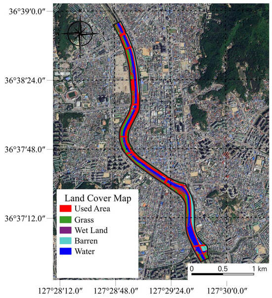
Figure 1.
Spatial structure of the study-area floodplain showing the distribution of land-cover types.
Spatial data were obtained from Sentinel-2 satellite imagery (10 m resolution) via the Copernicus Data Space Browser (https://browser.dataspace.copernicus.eu (accessed on 1 August 2025)). The Copernicus Programme jointly operated by the European Union, ESA, EUMETSAT, and participating member states constitutes an integrated Earth-observation infrastructure. Through its constellation of Sentinel satellites, in situ monitoring networks, and thematic services, Copernicus processes, stores, and distributes a vast volume of EO data via its core ground segment and collaborative hubs, providing stable access to Sentinel-2 optical imagery and a cloud-based processing environment that enables efficient acquisition and analysis of high-resolution datasets [40,41]. In this study, only images with less than 30% cloud cover from 2020 to 2024 were selected to construct the NDVI time series. Under the monsoon-driven weather conditions of the study watershed, persistent cloud cover often limited the availability of usable satellite images. To minimize this issue, we adopted the guideline suggested in [42] and applied a 30% cloud-coverage threshold when selecting scenes.
To minimize potential degradation that may occur when processing the entire area as a single extent, the study reach was subdivided into upper, middle, and lower sections for data acquisition and preprocessing (Figure 2).

Figure 2.
Preprocessing of Sentinel-2 imagery for NDVI analysis. (a) Original image before spatial clipping; (b) Extracted study-area floodplain after clipping.
Hydraulic data were generated using FaSTMECH (Flow and Sediment Transport with Morphological Evolution of Channels), a two-dimensional unsteady hydraulic model implemented within the International River Interface Cooperative (iRIC) platform. iRIC is an open-source, integrated modeling system capable of simulating diverse hydrological and hydraulic processes, including floods, rainfall–runoff, and geomorphic change [43]. FaSTMECH is based on the Reynolds-Averaged Navier–Stokes (RANS) equations and assumes incompressible, hydrostatic, quasi-steady flow conditions [44]. The model simulates in channel flow variations, sediment transport, and morphological evolution, making it suitable for riverine hydraulic analysis [45]. The model setup for this study including terrain data integration, mesh construction, and boundary condition assignment followed the methodological framework presented in earlier research [46]. Calibration of the model involved iteratively refining the Manning’s roughness values so that the simulated water depths and velocities aligned with the ADV observations obtained at six cross-sectional points. After calibration, the model was able to reproduce key hydraulic features, including backwater zones, accelerated flow near channel bends, and changes in inundation width. Using the same observational dataset for validation, the model showed strong agreement with measurements, with RMSE values of 0.0176 m for depth and 0.0160 m/s for velocity.
Hourly precipitation data from the Korea Meteorological Administration (KMA) ASOS network were used to classify rainfall intensity into four categories (light rain, moderate rain, heavy rain, and very heavy rain) according to official KMA criteria (Table 1). At the Cheongju station, the nearest to the study reach, the proportion of rainfall events was 17.0% light rain, 10.3% moderate rain, 1.4% heavy rain, and 0.5% very heavy rain. The maximum hourly rainfall recorded during the period was 54.9 mm, indicating that no extreme rainfall events occurred.

Table 1.
Classification of hourly rainfall intensity based on the criteria of the Korea Meteorological Administration (KMA).
2.2. NDVI Time-Series Processing and Variability Analysis
To quantify vegetation variability within the study reach, a time series of NDVI was constructed using Sentinel-2 multispectral imagery. NDVI was calculated using the reflectance values from the near-infrared band (Band 8; 10 m resolution) and the red band (Band 4), following the standard expression (Equation (1)). NDVI was calculated using the common expression (B08 − B04)/(B08 + B04), based on the 10-m red (B04) and near-infrared (B08) bands provided in the Sentinel-2 dataset. Because these products include atmospheric correction, variations caused by aerosols or water vapor are largely removed, and reflectance values remain comparable across different dates. With this preprocessing in place, the resulting NDVI time series reflects surface conditions in a consistent manner.
NDVI ranges from −1 to 1, with higher values indicating greater vegetation vigor and higher biomass. All images in the time series were resampled to a unified coordinate reference system and grid structure to ensure temporal consistency and spatial comparability across acquisition dates.
To evaluate vegetation sensitivity to rainfall, representative rainfall events during the analysis period were selected, and NDVI before and after each event (Before–After) was compared. By examining the changes in NDVI between the two time points, short-term vegetation responses to rainfall were assessed. Vegetation variability associated with rainfall events was quantified using the Coefficient of Variation (CV), as defined in Equation (2). The coefficient of variation is useful for comparing vegetation variability across the study floodplain, but it can respond strongly to outliers or short-term NDVI jumps, especially when cloud shadows or localized canopy disturbance occur. To reduce these effects, we removed scenes with cloud cover above 30% and manually checked the remaining images to filter values that were clearly inconsistent before calculating the variability metrics.
CV is a dimensionless index calculated by dividing the standard deviation of NDVI by its mean, where larger values indicate stronger relative sensitivity of vegetation to rainfall. After computing CV for each rainfall event, condition-specific mean CV values were derived to systematically evaluate NDVI fluctuation patterns and vegetation responsiveness under different rainfall intensities. As a relative measure of variability normalized by the mean, CV enables effective comparison of NDVI sensitivity across varying rainfall conditions.
2.3. Computation of Hydraulic Indices: SEDI and TEDI
In this study, the SEDI and the TEDI were computed to quantify erosion and deposition tendencies within the floodplain. These indices were derived from water depth, depth-averaged velocity (u), and bed shear stress (τ) outputs obtained from the FaSTMECH two-dimensional unsteady flow model. The computation followed the formulations and procedures proposed in previous research [47], incorporating variations in shear stress, flow velocity, acceleration (du/dt), and mean flow characteristics that collectively influence fluvial erosion and deposition.
SEDI evaluates long-term and average erosion–deposition tendencies based on the mean bed shear stress during a given flood wave, making it suitable for identifying relative depositional potential across floodplains. In contrast, TEDI utilizes the temporal rate of change in velocity (acceleration term) to identify localized, instantaneous erosion-prone areas under unsteady hydraulic conditions. This makes TEDI well-suited for representing the spatial distribution of transient erosion–deposition tendencies throughout the floodplain.
Together, these two indices provide complementary representations of steady and transient erosion–deposition dynamics under flood conditions. Accordingly, they were used as key indicators for assessing hydraulic effects and identifying potential zones of impact within the floodplain based on the model results.
SEDI and TEDI both span a 0–1 scale, with values near zero reflecting stronger erosional or depositional behavior. For comparison with the NDVI-based vegetation metrics, we rescaled the two indices within the range observed in the study reach and expressed them on the same 0–1 basis. This allowed the hydraulic and vegetation indicators to be placed on a common, dimensionless scale and made spatial comparison across the floodplain more straightforward.
In this study, SEDI and TEDI are used to characterize how susceptible each part of the floodplain is to hydraulic forcing, rather than to quantify actual geomorphic change. Since the hydraulic model had been evaluated through comparisons with field measurements, its outputs provide a credible basis for identifying areas where erosion or deposition is more likely to occur, even though direct sediment data were not available.
2.4. Spatial Interpolation
Because TEDI and SEDI are computed at discrete model grid points, converting these point-based indices into continuous raster surfaces is necessary to evaluate spatial patterns of erosion and deposition across the entire floodplain. To achieve this, three representative spatial interpolation methods Inverse Distance Weighting (IDW), Radial Basis Function (RBF), and Ordinary Kriging (Kriging) were applied to generate continuous spatial fields.
TEDI and SEDI values calculated at model grid points were used as input data for interpolation at a uniform spatial resolution. IDW estimates unknown values by computing a weighted average of nearby observations, where weights are inversely proportional to distance; it is widely used for spatial estimation due to its global applicability and strong ability to capture local patterns [48,49]. RBF interpolation constructs predictions using radial basis functions centered on sample points; its distance-based structure provides numerical stability and high-dimensional capability, making it effective even under complex geometries and boundary conditions [50,51,52]. Kriging, in contrast, models spatial autocorrelation to optimally estimate unknown values within a finite domain without bias. It performs probabilistic and local interpolation based on the variability of primary data without covariates and provides prediction variance, offering superior spatial estimation performance compared to deterministic methods [53,54,55].
To compare the spatial reliability of the three interpolation outcomes, Spatial K-Fold Cross-Validation was performed. Conventional random K-Fold methods ignore spatial autocorrelation and may yield overly optimistic accuracy, so this study employed a spatial block-based K-Fold approach that accounts for spatial dispersion. The entire set of model grid points was divided into K spatially separated blocks, and training-validation sets were generated iteratively for each fold. Interpolation accuracy was evaluated using root mean square error (RMSE), coefficient of determination (R2), Bias, and Spearman rank correlation (Table 2).
Table 2.
Performance Summary of Spatial Interpolation Methods.
3. Results
3.1. Changes in Floodplain Land Cover and Spatial Characteristics
Grass occupied the largest proportion of land cover in the floodplain at approximately 36.9%, followed by Used Area (23.6%) and Water (21.6%), indicating a heterogeneous landscape composed of vegetation, roadway areas, and river channels. In contrast, Agricultural Land accounted for only 0.1%, suggesting that the floodplain functions less as an agricultural zone and more as a space supporting recreation, waterfront activities, and ecological functions. This configuration forms a belt-shaped distribution of vegetation communities (Grass, Wet Land, Barren) with spatial continuity, providing conditions under which slight adjustments of the flow path may occur depending on hydrological fluctuations.
Vegetation density was notably higher along the left bank than on the right bank, consistent with the NDVI results showing larger variance in vegetation cover on the left bank (Figure 3). This structural heterogeneity contributes to asymmetry in flow velocity distribution during floods and increases the likelihood of erosion and deposition. Analysis of NDVI mean and standard deviation further revealed pronounced spatial heterogeneity. While NDVI mean values across most areas ranged from 0.4 to 0.7, indicating relatively stable vegetation, the outer bend locations exhibited standard deviation values exceeding 0.15, suggesting vegetation zones that are highly sensitive to seasonal and hydrological changes. In particular, regions with pronounced curvature displayed high NDVI variability, indicating persistent susceptibility to hydraulic disturbances such as cyclic erosion and deposition during flood events.
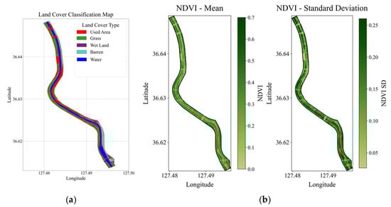
Figure 3.
Spatial analysis of land-cover structure and vegetation characteristics in the study floodplain. (a) Distribution of land-cover types, including Used Area, Agricultural Land, Forest, Grass, Wet Land, Barren, and Water; (b) Spatial patterns of mean NDVI and NDVI standard deviation, highlighting areas with high vegetation variability and sensitivity to hydrological fluctuations.
In grass dominated areas, the NDVI standard deviation reached 0.176, while wetland zones showed the largest spread at 0.200. These differences point to notable spatial irregularities in vegetation structure across the floodplain. Such variability can alter local hydraulic resistance, and areas with higher NDVI variation tend to experience more uneven inundation patterns and localized differences in shear stress during floods.
These findings clearly demonstrate that the floodplain is not a single-function space but rather a complex geomorphic environment where seasonal variability in vegetation vigor, the linear arrangement of waterfront facilities, and the meandering characteristics of the river channel overlap.
3.2. Vegetation Variability Assessment Based on the NDVI Time Series
Monthly-averaged Sentinel-2 NDVI values (Figure 4) show that while mean NDVI remains relatively stable across the study reach, variability is distinctly higher along the left bank. The spatial pattern indicates that vegetation along the left bank covers a broader area and exhibits stronger seasonal responsiveness compared to the right bank. NDVI variability, assessed using standard deviation, is concentrated along the left bank, suggesting the presence of zones where vegetation vigor is relatively unstable and more sensitive to hydrological fluctuations.
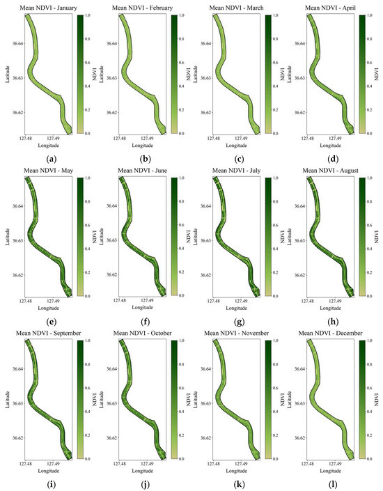
Figure 4.
Monthly spatial variation of NDVI across the study-area floodplain. (a) January; (b) February; (c) March; (d) April; (e) May; (f) June; (g) July; (h) August; (i) September; (j) October; (k) November; (l) December.
Variability is particularly pronounced in meander sections, where spatial gradients in NDVI become more evident. These areas are likely exposed to repeated cycles of erosion and deposition due to their hydraulic characteristics, leading to disruptions in the spatial continuity of vegetation cover. Moreover, the localized increases in standard deviation demonstrate that the floodplain does not function as a homogeneous ecological space but rather comprises segments with distinct and uneven vegetation stability.
Table 3 summarizes the observation periods before and after each case selected under different rainfall conditions. To minimize the influence of seasonal vegetation growth patterns on NDVI, the temporal window between the pre- and post-rainfall observations for all cases was restricted to within 30 days. The dormant season during which vegetation vigor declines significantly was excluded, and only data from the growing season (April to November) were used. This criterion was established to clearly capture the short-term effects of rainfall events on vegetation.
Table 3.
Observation periods for each case categorized by rainfall condition.
Classification of rainfall conditions was based on the cumulative rainfall recorded between the Before and After NDVI observations for each case. When cumulative rainfall exceeded 30 mm, the event was classified as Heavy rainfall; rainfall between 10 mm and 30 mm was classified as Moderate rainfall; rainfall of 10 mm or less was classified as Light rainfall; and 0 mm was classified as Dry conditions (Figure 5). This classification enables a quantitative comparison of the magnitude of NDVI responses to individual rainfall events and provides an essential basis for identifying spatial patterns in NDVI change and CV variation according to rainfall intensity.
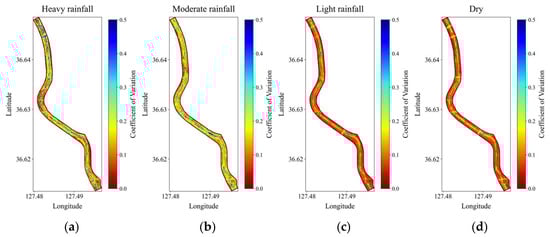
Figure 5.
Spatial distribution of NDVI coefficient of variation (CV) under different rainfall conditions. (a) Heavy rainfall; (b) Moderate rainfall; (c) Light rainfall; (d) Dry.
The CV for NDVI under different rainfall intensities showed that CV remained low under Dry and Light rainfall conditions, indicating that vegetation structure experienced minimal change. This suggests that small rainfall events are insufficient to induce direct disturbance to vegetation growth conditions. In contrast, under Moderate rainfall or stronger events, repeated fluctuations in NDVI were observed after rainfall, indicating reduced short-term resilience of vegetation cover and clearly expressed structural vulnerability. Variability was particularly pronounced in the downstream segment, likely because the lower reach is more frequently exposed to hydraulic disturbances such as flow concentration, lateral bank erosion, and changes in depositional patterns.
Additionally, certain meander sections and left-bank areas exhibited a proportional increase in CV with increasing rainfall intensity. This pattern indicates that these zones are inherently vulnerable geomorphic areas that remain sensitive to hydrological fluctuations even under normal flow conditions.
3.3. Spatial Characteristics of Erosion–Deposition Tendencies Based on SEDI and TEDI
The spatial distributions of SEDI and TEDI derived from the FaSTMECH hydraulic simulations exhibited distinct erosion and deposition tendencies across the upstream, midstream, and downstream sections of the study reach (Figure 6). In the upstream section, where flow velocities were relatively gentle and bed topography varied minimally, depositional tendencies dominated over a wide area. In contrast, the midstream section showed alternating patterns of erosion and deposition, resulting from the combined effects of channel-width transitions and increased curvature. This mixed pattern is interpreted as the outcome of flow deflection and changes in water-surface slope.

Figure 6.
Spatial distribution of erosion–deposition indices (SEDI and TEDI) across the study-area floodplain. (a) SEDI: Long-term/steady erosion–deposition tendencies; (b) TEDI: Instantaneous/transient erosion-prone zones.
In the downstream section, where the channel width narrows and localized high-velocity zones become more frequent, both SEDI and TEDI values increased, indicating a pronounced intensification of erosion. Higher index values were concentrated along the outer bends and near levee junctions, reflecting areas where hydraulic disturbances particularly the repeated erosion–deposition cycle are most active.
To secure reliability in the spatial distributions of SEDI and TEDI and to integrate these patterns with the spatial distribution of NDVI variability, cross-validation was conducted for the three interpolation methods applied (IDW, RBF, and Kriging) (Figure 7 and Figure 8). Under Random K-Fold validation, RBF demonstrated the lowest RMSE and highest R2, indicating the best overall predictive accuracy. However, under Spatial K-Fold validation, the spatial generalization ability of RBF declined substantially, whereas IDW exhibited the most stable RMSE, Bias, and Spearman ρ values, demonstrating relatively robust performance in areas with strong spatial heterogeneity (Figure 9 and Figure 10). Although Kriging effectively reproduced smoothed mean spatial patterns, it excessively flattened localized vulnerable zones, limiting its ability to detect spatially concentrated areas of risk.

Figure 7.
Comparison of SEDI interpolation results using three spatial interpolation methods. (a) IDW; (b) RBF; (c) Kriging.

Figure 8.
Comparison of TEDI interpolation results using three spatial interpolation methods. (a) IDW; (b) RBF; (c) Kriging.
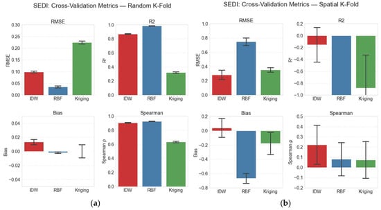
Figure 9.
Cross-validation results for SEDI interpolation using Random K-Fold and Spatial K-Fold methods. (a) Random K-Fold; (b) Spatial K-Fold.

Figure 10.
Cross-validation results for TEDI interpolation using Random K-Fold and Spatial K-Fold methods. (a) Random K-Fold; (b) Spatial K-Fold.
Therefore, for environments exhibiting high spatial heterogeneity such as reaches characterized by meandering, channel-width transitions, and localized flow concentration IDW is determined to be the most suitable interpolation method. IDW was selected not only for its stable performance in cross-validation but also for its ability to preserve sharp spatial gradients, which frequently occur near outer bends, constricted reaches, or areas of concentrated flow. Capturing these features is essential because erosion and deposition often develop in highly localized portions of the floodplain.
Kriging, by contrast, tended to oversmooth these transitions, and RBF occasionally produced unrealistic surface shapes in regions with sparse data. The IDW interpolations more closely reflected patterns commonly observed in river systems for example, elevated values along outer bends and reduced values toward inner banks indicating that the resulting surfaces provide a reasonable approximation of hydraulic tendencies. Nonetheless, we recognize that IDW can introduce artifacts where data availability is limited, and future efforts should explore the integration of physical constraints or advanced interpolation techniques to enhance spatial realism.
3.4. Environmental Safety Assessment Integrating NDVI CV, SEDI, and TEDI
The integrated environmental safety score combining the NDVI CV, SEDI, and TEDI under each rainfall condition ranged from 0.2 to 0.7, with higher values indicating greater safety. In the visualization, regions exceeding 0.7 were displayed in white to distinguish areas classified as highly stable (Figure 11). Across all rainfall conditions, a continuous band with values above 0.5 formed along the river axis, indicating generally stable conditions, while localized reductions in safety were observed primarily in specific meander sections.
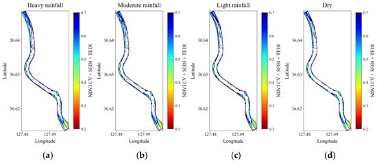
Figure 11.
Spatial patterns of environmental safety scores under varying rainfall conditions. (a) Heavy rainfall; (b) Moderate rainfall; (c) Light rainfall; (d) Dry.
Under Heavy rainfall conditions, integrated scores were predominantly within the 0.4–0.7 range, with continuous high-safety zones (≥0.7) appearing along the channel center and inner bank slopes. However, point-like clusters of values below 0.4 emerged in the upstream meander and in portions of the downstream outer bends, indicating that localized low-safety zones selectively develop under stronger rainfall conditions. The Moderate rainfall condition exhibited a spatial structure similar to that of Heavy rainfall, but with slightly fewer low-safety zones. A continuous band of 0.5–0.7 aligned with the riverflow direction, while regions below 0.4 appeared only in small portions near the upstream meander, becoming increasingly homogeneous toward the downstream section.
Under Light rainfall conditions, the extent of areas with scores between 0.5 and 0.7 expanded further. Values below 0.4 were limited to point-shaped patches mainly in the upstream meander and a few outer bends. Although the spatial locations of vulnerable zones were generally consistent with the heavier rainfall categories, their size and severity diminished. The Dry condition yielded the highest overall safety distribution among all four categories.
Comparing the four rainfall conditions reveals that scores above 0.5 consistently form a stable band along the channel axis, while low-safety zones persist primarily in the lower upstream meander and several outer bends. As rainfall intensity increases, these vulnerable zones expand modestly in area and distribution. Although the study reach is generally characterized by high environmental safety, the upstream meander and selected outer bends repeatedly exhibit low scores across multiple rainfall conditions, confirming these areas as structurally vulnerable zones that respond sensitively to hydrological disturbances.
4. Discussion
This study quantitatively evaluated the spatial safety of an urban river floodplain by integrating NDVI-based vegetation variability with erosion–deposition dynamics represented by SEDI and TEDI. This study does not interpret NDVI variability as a direct proxy for erosion risk. Rather, the coefficient of variation is employed to describe spatial contrasts in vegetation stability, and its combined use with hydraulically derived indicators such as SEDI and TEDI allows for improved identification of areas where hydrodynamic stress coincides with ecological sensitivity. Although geotechnical properties could not be incorporated due to limited data availability, the joint analysis of vegetation variability and hydraulic forcing provides a reconnaissance level perspective on floodplain susceptibility. The high NDVI variability observed along the left bank reflects vegetation disturbance driven by the combined influence of seasonality and localized hydrological fluctuations, corresponding structurally to the elevated TEDI and SEDI values that repeatedly appear along outer meander bends. This alignment indicates that areas vulnerable to hydraulic disturbances are also zones where vegetation stability is reduced, suggesting a heightened likelihood of long-term geomorphic change.
The objective of the study, is not to quantify the absolute magnitude of geomorphic change; rather, it is to delineate areas that are relatively more susceptible to erosion or deposition driven responses under varying hydraulic conditions. Because SEDI and TEDI are derived from shear stress and flow acceleration two governing variables in sediment entrainment they provide a meaningful basis for screening spatial patterns of vulnerability, especially in settings where high resolution geotechnical information is limited at the watershed scale. Incorporating spatially resolved soil properties or conducting targeted geotechnical field surveys would be a valuable direction for future work to enhance erosion–deposition assessments and extend their applicability to heterogeneous urban floodplains.
The interpolation comparison results, in which IDW demonstrated the most stable predictive performance under Spatial K-Fold validation, highlight that in highly heterogeneous riverine terrains, methods that preserve local spatial patterns are more appropriate than smoothing approaches such as Kriging. This finding underscores the importance of accurately reproducing local vulnerability zones in river management applications.
The integrated NDVI CV–SEDI–TEDI analysis under varying rainfall intensities revealed that low-safety zones expanded in the upstream meander and selected outer bends as rainfall increased, demonstrating the combined influence of rainfall events on both vegetation and hydraulic conditions. The occurrence of repeated low scores at the same locations under Dry and Light rainfall conditions further suggests that geometric vulnerability is intrinsically embedded in these sections.
This study evaluated rainfall events up to 54.9 mm/h, which represent moderate to strong storms within the region. The analysis was designed to examine how the floodplain responds under hydrological conditions that occur relatively frequently, rather than during rare, extreme flood events. We acknowledge that severe storms can activate additional processes notably bank failure, subsurface erosion or piping, and soil instability that fall outside the scope of the present framework. These mechanisms are critical for disaster risk reduction, and future scenario-based investigations that incorporate extreme hydrological and geotechnical conditions would provide a more comprehensive understanding of floodplain behavior during high impact events.
Future research should incorporate long-term erosion–deposition monitoring datasets, scenario-based projections of future safety under climate change, and integration with high-resolution data sources such as UAV and LiDAR to refine multifunctional management strategies for urban waterfront spaces.
5. Conclusions
This study assessed environmental safety in an urban river floodplain by integrating Sentinel-2 NDVI time series with the SEDI and TEDI indices derived from the FaSTMECH hydraulic model. The major findings are as follows:
- (1)
- The floodplain exhibits a heterogeneous spatial structure composed of vegetation, roadway areas, and river channels. Vegetation along the left bank shows higher variability, forming hydrologically sensitive zones susceptible to changes in flow conditions.
- (2)
- SEDI and TEDI exhibited a spatial gradient characterized by dominant deposition in the upstream section, mixed erosion–deposition patterns in the midstream section, and concentrated erosion in the downstream section. Recurrent local erosion risks were identified along outer meander bends.
- (3)
- Among the interpolation methods tested, IDW showed the best performance under Spatial K-Fold validation, confirming that methods preserving local spatial patterns are more suitable for river environments with strong spatial heterogeneity.
- (4)
- Integrated NDVI CV–SEDI–TEDI analysis showed that although most of the river axis maintains an environmental safety score above 0.5, the upstream meander and several outer bends repeatedly produced low scores as rainfall intensity increased, indicating structurally vulnerable zones.
This study provides scientific evidence to support effective use and spatial design of waterfront spaces developed within urban river floodplains and contributes to establishing spatial planning directions in river and urban design practice.
Author Contributions
Conceptualization, Y.D.K. and S.L.; methodology, S.L.; validation, J.K.; formal analysis, S.L.; investigation, S.L.; data curation, S.L. and J.K.; writing—original draft preparation, S.L. and J.K.; writing—review and editing, Y.D.K.; visualization, S.L.; supervision, Y.D.K.; funding acquisition, Y.D.K. All authors have read and agreed to the published version of the manuscript.
Funding
This work was funded by Korea Environment Industry & Technology Institute (KEITI) through Research and Development on the Technology for Securing the Water Resources Stability in Response to Future Change, funded by Korea Ministry of Climate, Energy, Environment (MCEE), grant number RS-2024-00397820.
Institutional Review Board Statement
Not applicable.
Informed Consent Statement
Not applicable.
Data Availability Statement
The datasets presented in this article are not readily available because they include results from an ongoing study and data acquired from areas managed by local governments, which are subject to restrictions. Requests to access the datasets should be directed to [ydkim@mju.ac.kr].
Conflicts of Interest
The authors declare no conflicts of interest. The funder had no role in the design of the study; in the collection, analyses, or interpretation of data; in the writing of the manuscript; or in the decision to publish the results.
Abbreviations
The following abbreviations are used in this manuscript:
| NDVI | Normalized Difference Vegetation Index |
| FaSTMECH | Flow and Sediment Transport with Morphological Evolution of Channels |
| TEDI | Transient Erosion and Deposition Index |
| SEDI | Steady Erosion and Deposition Index |
| CV | Coefficient of Variation |
| IDW | Inverse Distance Weighting |
| RBF | Radial Basis Function |
| RMSE | Root Mean Square Error |
References
- Wang, K.; Fang, C. Revealing the synergy between carbon reduction and pollution control in the process of new-type urbanization: Evidence from China’s five major urban agglomerations. Sustain. Cities Soc. 2025, 120, 106154. [Google Scholar] [CrossRef]
- Zhang, H.; Nijhuis, S.; Newton, C.; Tao, Y. Healthy urban blue space design: Exploring the associations of blue space quality with recreational running and cycling using crowdsourced data. Sustain. Cities Soc. 2024, 117, 105929. [Google Scholar] [CrossRef]
- Ortega, E.; Martín, B.; LÓPez-Lambas, M.E.; Soria-Lara, J.A. Evaluating the impact of urban design scenarios on walking accessibility: The case of the Madrid ‘Centro’district. Sustain. Cities Soc. 2021, 74, 103156. [Google Scholar] [CrossRef]
- Gao, W.; Qian, Y.; Chen, H.; Zhong, Z.; Zhou, M.; Aminpour, F. Assessment of sidewalk walkability: Integrating objective and subjective measures of identical context-based sidewalk features. Sustain. Cities Soc. 2022, 87, 104142. [Google Scholar] [CrossRef]
- Kim, Y.; Yeo, H.; Lim, L. Sustainable, walkable cities for the elderly: Identification of the built environment for walkability by activity purpose. Sustain. Cities Soc. 2024, 100, 105004. [Google Scholar] [CrossRef]
- Huang, Z.; Liu, Y.; Pan, C.; Wang, Y.; Yu, H.; He, W. Energy-saving effects of yard spaces considering spatiotemporal activity patterns of rural Chinese farm households. J. Clean. Prod. 2022, 355, 131843. [Google Scholar] [CrossRef]
- Qiao, S.; Yeh, A.G.O. Understanding the effects of environmental perceptions on walking behavior by integrating big data with small data. Landsc. Urban Plan. 2023, 240, 104879. [Google Scholar] [CrossRef]
- Remme, R.P.; Frumkin, H.; Guerry, A.D.; King, A.C.; Mandle, L.; Sarabu, C.; Bratman, G.N.; Giles-Corti, B.; Hamel, P.; Han, B.; et al. An ecosystem service perspective on urban nature, physical activity, and health. Proc. Natl. Acad. Sci. USA 2021, 118, e2018472118. [Google Scholar] [CrossRef]
- Vian, F.D.; Izquierdo, J.J.P.; Martínez, M.S. River-city recreational interaction: A classification of urban riverfront parks and walks. Urban For. Urban Green. 2021, 59, 127042. [Google Scholar] [CrossRef]
- Mishra, H.S.; Bell, S.; Vassiljev, P.; Kuhlmann, F.; Niin, G.; Grellier, J. The development of a tool for assessing the environmental qualities of urban blue spaces. Urban For. Urban Green. 2020, 49, 126575. [Google Scholar] [CrossRef]
- Elliott, L.R.; White, M.P.; Taylor, A.H.; Herbert, S. Energy expenditure on recreational visits to different natural environments. Soc. Sci. Med. 2015, 139, 53–60. [Google Scholar] [CrossRef] [PubMed]
- Naiman, R.J.; Decamps, H. The ecology of interfaces: Riparian zones. Annu. Rev. Ecol. Syst. 1997, 28, 621–658. [Google Scholar] [CrossRef]
- Yi, X.; Huang, Y.; Ma, M.; Wen, Z.; Chen, J.; Chen, C.; Wu, S. Plant trait-based analysis reveals greater focus needed for mid-channel bar downstream from the Three Gorges Dam of the Yangtze River. Ecol. Indic. 2020, 111, 105950. [Google Scholar] [CrossRef]
- Zheng, J.; Arif, M.; Zhang, S.; Yuan, Z.; Zhang, L.; Li, J.; Ding, D.; Li, C. Dam inundation simplifies the plant community composition. Sci. Total Environ. 2021, 801, 149827. [Google Scholar] [CrossRef]
- Völker, S.; Kistemann, T. The impact of blue space on human health and well-being–Salutogenetic health effects of inland surface waters: A review. Int. J. Hyg. Environ. Health 2011, 214, 449–460. [Google Scholar] [CrossRef]
- Higgins, S.L.; Thomas, F.; Goldsmith, B.; Brooks, S.J.; Hassall, C.; Harlow, J.; Stone, D.; Völker, S.; White, P. Urban freshwaters, biodiversity, and human health and well-being: Setting an interdisciplinary research agenda. Wiley Interdiscip. Rev. Water 2019, 6, e1339. [Google Scholar] [CrossRef]
- Gurnell, A.; Lee, M.; Souch, C. Urban rivers: Hydrology, geomorphology, ecology and opportunities for change. Geogr. Compass 2007, 1, 1118–1137. [Google Scholar] [CrossRef]
- Davis, J.; O’Grady, A.P.; Dale, A.; Arthington, A.H.; Gell, P.A.; Driver, P.D.; Bond, N.; Casanova, M.; Finlayson, M.; Watts, R.J.; et al. When trends intersect: The challenge of protecting freshwater ecosystems under multiple land use and hydrological intensification scenarios. Sci. Total Environ. 2015, 534, 65–78. [Google Scholar] [CrossRef]
- Smith, R.F.; Hawley, R.J.; Neale, M.W.; Vietz, G.J.; Diaz-Pascacio, E.; Herrmann, J.; Lovell, A.C.; Prescott, C.; Rios-Touma, B.; Smith, B.; et al. Urban stream renovation: Incorporating societal objectives to achieve ecological improvements. Freshw. Sci. 2016, 35, 364–379. [Google Scholar] [CrossRef]
- De Bell, S.; Graham, H.; White, P.C. Evaluating dual ecological and well-being benefits from an urban restoration project. Sustainability 2020, 12, 695. [Google Scholar] [CrossRef]
- McCormick, A.; Fisher, K.; Brierley, G. Quantitative assessment of the relationships among ecological, morphological and aesthetic values in a river rehabilitation initiative. J. Environ. Manag. 2015, 153, 60–67. [Google Scholar] [CrossRef]
- Tribot, A.S.; Deter, J.; Mouquet, N. Integrating the aesthetic value of landscapes and biological diversity. Proc. R. Soc. B Biol. Sci. 2018, 285, 20180971. [Google Scholar] [CrossRef] [PubMed]
- Aboufazeli, S.; Jahani, A.; Farahpour, M. Aesthetic quality modeling of the form of natural elements in the environment of urban parks. Evol. Intell. 2024, 17, 327–338. [Google Scholar] [CrossRef]
- Pekel, J.F.; Cottam, A.; Gorelick, N.; Belward, A.S. High-resolution mapping of global surface water and its long-term changes. Nature 2016, 540, 418–422. [Google Scholar] [CrossRef] [PubMed]
- Pickens, A.H.; Hansen, M.C.; Hancher, M.; Stehman, S.V.; Tyukavina, A.; Potapov, P.; Marroquin, B.; Sherani, Z. Mapping and sampling to characterize global inland water dynamics from 1999 to 2018 with full Landsat time-series. Remote Sens. Environ. 2020, 243, 111792. [Google Scholar] [CrossRef]
- Pander, J.; Knott, J.; Mueller, M.; Geist, J. Effects of environmental flows in a restored floodplain system on the community composition of fish, macroinvertebrates and macrophytes. Ecol. Eng. 2019, 132, 75–86. [Google Scholar] [CrossRef]
- Rogers, J.S.; Maneta, M.P.; Sain, S.R.; Madaus, L.E.; Hacker, J.P. The role of climate and population change in global flood exposure and vulnerability. Nat. Commun. 2025, 16, 1287. [Google Scholar] [CrossRef]
- Tellman, B.; Sullivan, J.A.; Kuhn, C.; Kettner, A.J.; Doyle, C.S.; Brakenridge, G.R.; Erickson, T.A.; Slayback, D.A. Satellite imaging reveals increased proportion of population exposed to floods. Nature 2021, 596, 80–86. [Google Scholar] [CrossRef]
- Devitt, L.; Neal, J.; Coxon, G.; Savage, J.; Wagener, T. Flood hazard potential reveals global floodplain settlement patterns. Nat. Commun. 2023, 14, 2801. [Google Scholar] [CrossRef]
- Kuo, N.W.; Jien, S.H.; Hong, N.M.; Chen, Y.T.; Lee, T.Y. Contribution of urban runoff in Taipei metropolitan area to dissolved inorganic nitrogen export in the Danshui River, Taiwan. Environ. Sci. Pollut. Res. 2017, 24, 578–590. [Google Scholar] [CrossRef]
- Kumar, B.; Verma, V.K.; Mishra, M.; Piyush; Kakkar, V.; Tiwari, A.; Kumar, S.; Yadav, V.P.; Gargava, P. Assessment of persistent organic pollutants in soil and sediments from an urbanized flood plain area. Environ. Geochem. Health 2021, 43, 3375–3392. [Google Scholar] [CrossRef] [PubMed]
- Gao, Z.; Zhang, Q.; Li, J.; Wang, Y.; Dzakpasu, M.; Wang, X.C. First flush stormwater pollution in urban catchments: A review of its characterization and quantification towards optimization of control measures. J. Environ. Manag. 2023, 340, 117976. [Google Scholar] [CrossRef] [PubMed]
- Manning, P.; Van Der Plas, F.; Soliveres, S.; Allan, E.; Maestre, F.T.; Mace, G.; Whittingham, M.J.; Fischer, M. Redefining ecosystem multifunctionality. Nat. Ecol. Evol. 2018, 2, 427–436. [Google Scholar] [CrossRef]
- Wohl, E. An integrative conceptualization of floodplain storage. Rev. Geophys. 2021, 59, e2020RG000724. [Google Scholar] [CrossRef]
- Alsdorf, D.E.; Rodríguez, E.; Lettenmaier, D.P. Measuring surface water from space. Rev. Geophys. 2007, 45. [Google Scholar] [CrossRef]
- Huang, C.; Chen, Y.; Zhang, S.; Wu, J. Detecting, extracting, and monitoring surface water from space using optical sensors: A review. Rev. Geophys. 2018, 56, 333–360. [Google Scholar] [CrossRef]
- Papa, F.; Frappart, F. Surface water storage in rivers and wetlands derived from satellite observations: A review of current advances and future opportunities for hydrological sciences. Remote Sens. 2021, 13, 4162. [Google Scholar] [CrossRef]
- Li, M.; Liu, J.; Xia, Y. Risk prediction of gas hydrate formation in the wellbore and subsea gathering system of deep-water turbidite reservoirs: Case analysis from the south China Sea. Reserv. Sci. 2025, 1, 52–72. [Google Scholar] [CrossRef]
- Cao, L.; Lv, M.; Li, C.; Sun, Q.; Wu, M.; Xu, C.; Dou, J. Effects of crosslinking agents and reservoir conditions on the propagation of fractures in coal reservoirs during hydraulic fracturing. Reserv. Sci. 2025, 1, 36–51. [Google Scholar] [CrossRef]
- Storch, T.; Reck, C.; Holzwarth, S.; Wiegers, B.; Mandery, N.; Raape, U.; Strobl, C.; Volkmann, R.; Böttcher, M.; Hirner, A.; et al. Insights into CODE-DE–Germany’s Copernicus data and exploitation platform. Big Earth Data 2019, 3, 338–361. [Google Scholar] [CrossRef]
- Hagos, D.H.; Kakantousis, T.; Vlassov, V.; Sheikholeslami, S.; Wang, T.; Dowling, J.; Paris, C.; Marinelli, D.; Weikmann, G.; Bruzzone, L.; et al. ExtremeEarth meets satellite data from space. IEEE J. Sel. Top. Appl. Earth Obs. Remote Sens. 2021, 14, 9038–9063. [Google Scholar] [CrossRef]
- Corbane, C.; Politis, P.; Kempeneers, P.; Simonetti, D.; Soille, P.; Burger, A.; Pesaresi, M.; Sabo, F.; Syrris, V.; Kemper, T. A global cloud free pixel-based image composite from Sentinel-2 data. Data Brief 2020, 31, 105737. [Google Scholar] [CrossRef] [PubMed]
- Hosseiny, H. A deep learning model for predicting river flood depth and extent. Environ. Model. Softw. 2021, 145, 105186. [Google Scholar] [CrossRef]
- Sansom, B.J.; Call, B.C.; Legleiter, C.J.; Jacobson, R.B. Performance evaluation of a channel rehabilitation project on the Lower Missouri River and implications for the dispersal of larval pallid sturgeon. Ecol. Eng. 2023, 194, 107045. [Google Scholar] [CrossRef]
- Shimizu, Y.; Nelson, J.; Arnez Ferrel, K.; Asahi, K.; Giri, S.; Inoue, T.; Iwasaki, T.; Jang, C.; Kang, T.; Kimura, I.; et al. Advances in computational morphodynamics using the International River Interface Cooperative (iRIC) software. Earth Surf. Process. Landf. 2020, 45, 11–37. [Google Scholar] [CrossRef]
- Kim, J.; Ku, T.G.; Lee, S.; Ok, G.; Kim, Y.D. Application of Hydraulic Safety Evaluation Indices to Waterfront Facilities in Floodplains. Appl. Sci. 2025, 15, 11627. [Google Scholar] [CrossRef]
- Song, C.G.; Ku, T.G.; Kim, Y.D.; Park, Y.S. Floodplain stability indices for sustainable waterfront development by spatial identification of erosion and deposition. Sustainability 2017, 9, 735. [Google Scholar] [CrossRef]
- Liu, Y.; Qian, Y.; Zhu, Y.; Xu, W.; Wei, G.; Huang, J.; Qiao, Y.; Ma, Q. Spatial estimation of large-scale soil salinity using enhanced inverse distance weighting method and identifying its driving factors. Agric. Water Manag. 2025, 317, 109645. [Google Scholar] [CrossRef]
- Kearney, K.M.; Harley, J.B.; Nichols, J.A. Inverse distance weighting to rapidly generate large simulation datasets. J. Biomech. 2023, 158, 111764. [Google Scholar] [CrossRef]
- Lin, C.C.; Lin, Y.C.; Cheng, C.W.; Tsai, M.C. Enhancing measurement efficiency for 3D printed magnet through radial basis function interpolation. J. Magn. Magn. Mater. 2024, 602, 172192. [Google Scholar] [CrossRef]
- Wang, Y.; Yuan, F.; Cammarano, D.; Liu, X.; Tian, Y.; Zhu, Y.; Cao, W.; Cao, Q. Integrating machine learning with spatial analysis for enhanced soil interpolation: Balancing accuracy and visualization. Smart Agric. Technol. 2025, 11, 101032. [Google Scholar] [CrossRef]
- He, B.; He, X.; Chen, M. Solving parabolic partial differential equations via hybrid radial basis functions with the Adam optimization algorithm. Eng. Anal. Bound. Elem. 2025, 179, 106391. [Google Scholar] [CrossRef]
- Kumar, A.; Mishra, R.K.; Sarma, K. Mapping spatial distribution of traffic induced criteria pollutants and associated health risks using kriging interpolation tool in Delhi. J. Transp. Health 2020, 18, 100879. [Google Scholar] [CrossRef]
- Guisande, C.; Rueda-Quecho, A.J.; Rangel-Silva, F.A.; Heine, J.; García-Roselló, E.; González-Dacosta, J.; González-Vilas, L.; Pelayo-Villamil, P. SINENVAP: An algorithm that employs kriging to identify optimal spatial interpolation models in polygons. Ecol. Inform. 2019, 53, 100975. [Google Scholar] [CrossRef]
- Ling, J.; Yang, D.; Liu, C.; Gong, W. A novel boundary meshfree method with two kinds of interpolations for spatially varying coefficient orthotropic thermal transfer. Case Stud. Therm. Eng. 2025, 72, 106455. [Google Scholar] [CrossRef]
Disclaimer/Publisher’s Note: The statements, opinions and data contained in all publications are solely those of the individual author(s) and contributor(s) and not of MDPI and/or the editor(s). MDPI and/or the editor(s) disclaim responsibility for any injury to people or property resulting from any ideas, methods, instructions or products referred to in the content. |
© 2025 by the authors. Licensee MDPI, Basel, Switzerland. This article is an open access article distributed under the terms and conditions of the Creative Commons Attribution (CC BY) license.