Featured Application
The proposed BIM-Machine Learning framework applies to early-stage assessment of building energy performance, providing an expeditious data-driven approach to support sustainable design decision-making.
Abstract
A Building Information Modeling (BIM)-based Machine Learning (ML) framework was developed to predict the energy performance of office buildings at the early design stage. The framework provides a reproducible and data-driven workflow that shortens simulation time while maintaining accuracy. Revit and Insight were integrated with statistical modeling in Weka to create an automated and regionally adaptable process derived from BIM-generated data. A reduced-factorial Design of Experiments (DOE) guided the generation of 210 parametric simulations representing base, generalization, and stress-test models for Orlando, Florida. Each model combined geometric, envelope, system, and operational variations, forming a dataset of 14 independent parameters and two dependent energy metrics: Energy Use Intensity (EUI) and Operational Energy (OE). Four regression algorithms—Linear Regression (LR), M5P, SMOReg, and Random Forest (RF)—were trained and validated through 10-fold cross-validation. All models achieved R2 values above 0.95, with the RF model reaching the highest overall accuracy under default parameter settings, with R2 > 0.97 and mean absolute errors below 5% across both metrics, EUI and OE. Feature-importance analysis identified HVAC system type, window-to-wall ratio, and operational schedule as the most influential variables. Results confirm that BIM-ML integration enables rapid and reliable energy-performance prediction, supporting informed, energy-efficient design decisions in the earliest phases of the building lifecycle.
1. Introduction
Building energy consumption used for heating, cooling, ventilation, and lighting has a direct impact on the environment because most electricity is still produced from fossil fuels—coal, natural gas, petroleum, and other gases [1,2]. The extraction, conversion, and combustion of these fuels to supply the energy releases large amounts of greenhouse gases, contributing to global warming and ecosystem degradation. For this reason, building energy performance evaluation is fundamental in sustainable design for conscious decision-making.
As the construction sector faces the challenge to reduce energy demands throughout the building life cycle, architects and engineers require tools capable of providing rapid, accurate, and interpretable feedback at the earliest design stages. Traditional simulation techniques, while precise, are often data-intensive and lag behind for practical use during the conceptual phase, when multiple options are reviewed and revised.
In response, recent research has shifted toward data-driven approaches that leverage Building Information Modeling (BIM) and Machine Learning (ML) to automate prediction, reduce analysis time, and enhance decision support. This section provides an overview of the state of knowledge in building-energy assessment, covering traditional simulation methods, statistical and ML-based models, BIM integration, and uncertainty management. It concludes by identifying the research gap that motivates the present study.
1.1. Overview of State of Knowledge
The building sector plays a pivotal role in achieving global sustainability goals, accounting for approximately 34% of total final energy demand and 37% of energy and process-related carbon dioxide (CO2) emissions [3]. Due to continued urbanization and construction growth, early-stage design decisions have a major relevance on long-term energy performance.
Building Performance Simulation (BPS) tools—such as EnergyPlus (v9.6.0), DesignBuilder (v6.1.8.021), and eQuest (v3.65build7175)—model heat transfer, HVAC system operation, and lighting loads to estimate energy consumption and efficiency [4]. Although they provide accurate results, their high data and computational requirements make them impractical during conceptual design, where multiple iterations must be explored rapidly.
Integrating BIM, such as Autodesk Revit (2024), and analysis engines, such as Autodesk Insight Carbon Analysis (2023.1), has improved workflow accessibility and collaboration. However, even BIM-linked simulations remain iterative and time-consuming, limiting their scalability. This context has motivated the use of ML models that can learn patterns from simulation or measured data to predict building energy use with minimal input, offering faster and more responsive evaluation for early-stage decision making.
1.2. Energy Assessment Approaches
Energy-performance assessment methods are typically categorized as engineering, simulation, and statistical approaches [5].
Engineering and simulation models provide high-fidelity analysis by explicitly describing thermodynamic and mechanical system interactions. However, their complexity and data demands constrain their applicability in conceptual design.
To reduce computational effort, statistical regression models have been applied to identify empirical relationships between design variables and energy use. Regression techniques can effectively capture overall consumption trends but generally fail to represent nonlinear dependencies among multiple design parameters [6].
Researchers have increasingly adopted data-driven models capable of describing complex, nonlinear relationships between building-design features and energy performance without relying on explicit physical equations.
1.3. Machine Learning for Building Energy Prediction
ML offers strong potential for accelerating building energy evaluation through predictive modeling. Early studies applied Artificial Neural Network (ANN) to model building thermal behavior, demonstrating that data-driven models can approximate simulation outputs with high accuracy [7]. Additional supervised algorithms, including Support Vector Machine (SVM) and Random Forest (RF), have been widely explored for energy forecasting.
Ahmad et al. [8] reported Mean Absolute Error (MAE) values below 10% when predicting building energy consumption using ANN and SVM, while Duarte et al. [9] confirmed that both methods outperform linear regression for nonlinear datasets. Ensemble methods such as RF have shown outstanding performance and robustness: Wang et al. [10] achieved a statistical performance indicator—Coefficient of Determination (R2)—near 0.95, with minimal parameter tuning, and Walker et al. [11] demonstrated that RF maintains high predictive accuracy across different temporal resolutions.
Feature-importance analysis from RF models provides valuable insights for design decision-making, identifying HVAC efficiency, envelope U-value, glazing ratio, and orientation as the most influential parameters affecting annual Energy Use Intensity (EUI) [11,12].
Comprehensive reviews [5,13] confirm that ML can reach simulation-level accuracy with up to 90% less computation time. More recent research has also integrated ML with optimization algorithms to enhance prediction and automate parameter tuning during design-space exploration [14,15].
1.4. BIM-Based Data Generation and Integration with Machine Learning
Accurate ML prediction depends on high-quality, structured data, an advantage provided by BIM, which encodes geometry, materials, and system information within a coordinated digital model [16]. BIM facilitates automatic extraction of energy-relevant features such as window-to-wall (WWR) and lighting power density (LPD), enabling the creation of consistent datasets for ML training.
Ma, Liu & Shang [17] developed a BIM-ANN plug-in that generated real-time energy-performance feedback, while Pan et al. [18] and Khan et al. [19] reviewed BIM-ML frameworks and confirmed that integration accelerates sustainability evaluation. However, Hollberg et al. [20] identified persistent challenges related to interoperability, data exchange formats, and the scarcity of open BIM-energy repositories.
Despite these obstacles, coupling BIM and ML offers two critical advantages: (1) generation of parametric datasets for model training and (2) embedding of predictive analytics directly within design workflows—key goals addressed in this study.
1.5. Managing Uncertainty in the Early-Design Stage
The conceptual design phase involves high uncertainty regarding geometry, material properties, and operational schedules. Traditional simulations handle this variability poorly, as each design adjustment requires a new computation.
Ning & You [21] proposed using ML and parametric modeling to explore uncertain design spaces automatically, while Feng, Lu & Wang [22] demonstrated that parametric-ML frameworks quantify sensitivity and identify critical design parameters affecting energy use.
BIM’s parametric capabilities make it possible to generate synthetic datasets, with controlled variations of design attributes and corresponding simulated outputs, to train ML models that remain reliable across diverse configurations.
D’Amico et al. [23] emphasized the need for such structured datasets to overcome data scarcity and improve model generalization.
This approach forms the methodological foundation for the present research, which employs BIM-generated simulations to train surrogate ML models capable of predicting EUI and Operational Energy (OE) efficiently under early-stage uncertainty.
1.6. Research Gap and Motivation
The reviewed literature illustrates a clear evolution from physics-based simulation to BIM-enabled, ML-assisted energy prediction. However, several limitations persist:
- Data scarcity and standardization: open, validated BIM-energy datasets for ML training remain limited, reducing reproducibility and comparative analysis across studies [20];
- Workflow integration: most ML approaches rely on external preprocessing, requiring users to export and format simulation outputs before training or prediction, since real-time evaluation within BIM platforms is still underdeveloped [19]; and
- Model transparency: many ML algorithms function as “black boxes,” providing accurate predictions but offering limited interpretability for architects and engineers during design decision-making [24].
Addressing these challenges, this study proposes a BIM-based ML framework that bridges simulation and prediction through structured data generation and external supervised learning. The approach integrates Revit and Insight simulations with ML modeling in Weka to predict EUI and OE during the early design stage. Although the workflow requires data preprocessing outside the BIM environment, it establishes a reproducible, adaptable method that enables designers to use simulation results directly in surrogate energy models.
By combining the accuracy of simulation with the efficiency of ML, the framework accelerates early-stage sustainability evaluation, enhances understanding of parameter influence, and supports informed architectural decision-making for energy-efficient office buildings.
Despite the growing interest in integrating BIM and ML for building energy prediction, existing workflows continue to face significant interoperability challenges. Common limitations include inconsistent data schemas between BIM platforms and ML environments, the absence of seamless native data exchange requiring intermediary data handling, loss of semantic information during export, and limited bidirectional data exchange. These issues often introduce preprocessing uncertainty and reduce reproducibility across platforms. In addition, prior studies employ a wide range of ML algorithms under heterogeneous conditions, with limited discussion on their suitability for different data structures. Linear models are typically applied to small, well-behaved datasets but struggle with nonlinearity, whereas tree-based and ensemble models offer improved performance at the expense of interpretability and higher data requirements. However, few studies explicitly analyze these trade-offs in relation to dataset structure, parameter interaction, and generalization capability.
Beyond these general limitations, substantial structural challenges remain in the transformation of BIM data for use in predictive modeling.
Although previous studies have integrated BIM and ML for building energy prediction [5,13,16], most existing frameworks rely on either unstructured simulation datasets, limited robustness testing, or partial methodological disclosure, which restricts reproducibility and generalization. Furthermore, few studies explicitly document statistically balanced reduced-factorial Design of Experiments (DOE) [25,26] construction, boundary stress-testing, and full dataset replication protocols within a BIM-driven workflow [5,13].
Compared with existing BIM-ML frameworks such as those reported in the literature [17,18,19], which typically focus on single-case parametric dataset generation or tool-specific BIM-ML plug-in implementations, the present study adopts a statistically structured experimental design that explicitly targets generalizability and reproducibility. While prior studies demonstrate the feasibility of BIM-ML coupling for energy prediction, they often rely on limited parameter spaces, non-balanced datasets, or case-specific workflows that restrict external validation. In contrast, this study formalizes the data-generation process through a reduced-factorial DOE, integrates systematic dataset expansion and stress-testing, and provides a fully documented replication protocol. These methodological differences position the proposed framework as a generalizable research infrastructure rather than a single-application BIM-ML implementation.
This study uniquely contributes by (i) establishing a fully documented reduced-factorial BIM-based experimental design, (ii) integrating systematic dataset expansion and stress-testing for robustness verification, and (iii) providing an open, reproducible BIM-ML dataset with full procedural transparency. These contributions distinguish the proposed framework from prior BIM-ML implementations and directly address data scarcity, reproducibility, and methodological rigor.
It is essential to distinguish between model generalization and framework generalizability. The surrogate models presented in this study are deliberately trained for a specific building typology (office), and climatic context (ASHRAE Climate Zone 2A) [27], and no claim is made regarding their direct transferability beyond these bounds. In contrast, the proposed BIM–ML framework is intrinsically typology- and region-agnostic. The reduced-factorial DOE [25,26], BIM-driven parameterization, and machine-learning training workflow together define a systematic and reproducible methodology that can be straightforwardly extended to other building types and climates through redefinition of input ranges and retraining using context-specific simulation data. The primary contribution of this work is therefore not a universally applicable predictive model, but a robust, generalizable framework for generating reliable early-stage surrogate models across diverse design contexts.
2. Materials and Methods
The workflow developed for this study integrated Revit for geometric and locational modeling, Insight for parametric energy simulation and data generation, and Weka for statistical analysis and ML. This combination established a transparent, repeatable, and adaptable data-driven process linking BIM-based modeling with predictive analytics for early-stage building design.
2.1. Research Design
A reduced-factorial DOE [25,26] was adopted to systematically vary key building design parameters while maintaining statistical efficiency and minimizing computational effort. This approach enabled the exploration of geometric, envelope, system, and operational variations without the exponential growth in runs associated with a full-factorial design.
The reduced-factorial method preserved the essential DOE principles of level balance, approximate orthogonality, and sufficient degrees of freedom to estimate main effects and selected interactions.
A total of 210 parametric building models were generated and organized into three experimental stages:
- 168 base models, representing the principal combination of design parameters;
- 32 generalization models, expanding the dataset to include additional parameter interactions; and
- 10 stress-test models, evaluating robustness under extreme design and operational conditions.
Each model represented a unique configuration capturing the combined effects of early-stage design decisions on building energy performance. All simulations corresponded to Orlando, Florida (ASHRAE Climate Zone 2A) [27], representative of warm-humid climates.
2.2. Experimental Parameters and Levels
The experimental framework considered 11 independent parameters corresponding to dominant architectural and operational variables influencing building energy performance: shape, orientation, HVAC system, infiltration rate, LPD, operation schedule, plug loads, and WWR for each façade (North, East, South, and West).
Other aspects, such as building lifespan (20 years) and emission factor (0.45 kg CO2e/kWh), were held constant to ensure consistency across all simulations. Additionally, the gross floor area (GFA) was kept within a narrow range of approximately 27,000–31,000 ft2 among all prototypes to guarantee geometric comparability and isolate the effects of shape and parameter variations rather than scale differences.
Although Insight provides a broad range of default parameter options, the number of levels per factor was intentionally limited to maintain statistical balance, reduce computational complexity, and ensure that each selected level represented realistic and distinct design conditions for contemporary office buildings in a warm-humid climate.
Specifically, HVAC systems uncommon for this building typology (e.g., radiant floor, evaporative cooling, district chilled water) were excluded, and upper limits were imposed on infiltration (≤0.12 CFM/ft2) and LPD (≤1.00 W/ft2).
Operation schedules were narrowed to three representative modes—8 a.m.–5 p.m., 12/5, and 24/7—capturing typical, extended, and continuous operations.
As summarized in Table 1, the selected parameters exhibited unequal numbers of levels (7, 4, 4, 3, 3, 3, 2, 3, 3, 3, 3), which would yield a theoretical 1,632,960 possible combinations under a full-factorial design before reduction.

Table 1.
Experimental parameters and corresponding levels used in the reduced-factorial design.
2.3. Reduced-Factorial Framework
To maintain statistical efficiency while avoiding the exponential growth of a full-factorial design, a custom reduced-factorial framework was developed in Microsoft Excel.
The final run size (N = 168) provided balanced representation across all 11 factors and was divisible by the major level counts (7, 4, 3, 2), ensuring sufficient coverage of the design space while remaining computationally feasible for Revit-Insight simulations.
Two coupling constraints were enforced to maintain architectural realism:
- HVAC-orientation applicability, restricting system-orientation pairs to realistic combinations (e.g., 0°/45° with GSHP w/DOAS + ERV; 90°/180° with VAV w/WC systems).
- Façade WWR coordination, limited to nine predefined glazing patterns (e.g., [0, 0, 0, 0], [30, 30, 30, 30], [50, 50, 50, 50]) to ensure practical design coherence.
Level balance and approximate orthogonality were verified through iterative frequency checks, ensuring deviations remained within ±12 runs per level.
The Excel-constructed reduced-factorial matrix served as the master input schedule for Revit-Insight simulations.
The reduced-factorial DOE [25,26] was selected over optimization-based sampling methods (e.g., D-optimal and Bayesian optimization [28,29]) because the objective of this study was not design optimization, but rather the construction of a statistically balanced, replication-ready training dataset for supervised ML. Optimization-based DOE methods prioritize convergence toward optimal solutions but do not guarantee uniform level representation or transparency for surrogate-model training. In contrast, the reduced-factorial approach ensured controlled coverage of mixed-level parameters, replicability across BIM platforms, and direct interpretability of factor effects, which are essential for ML generalization studies at the conceptual design stage.
Orthogonality was assessed at the practical level through systematic inspection of marginal frequency distributions and factor co-occurrence patterns, rather than formal algebraic D-efficiency metrics [26,28], which is appropriate given the study objective of balanced surrogate-model training rather than numerical optimization.
2.4. Dataset Expansion and Stress Testing
After the first ML training with the 168 initial models, to enhance the statistical diversity and generalization capacity of the dataset, the 168-run base design was expanded by 32 generalization models (M-169 to M-200). These additional configurations preserved established coupling and façade-pattern rules while improving marginal balance among underrepresented levels.
Furthermore, 10 stress-test models (M-201 to M-210) were created to evaluate robustness under boundary conditions.
Five high-load cases combined elevated internal and envelope demands—LPD = 1.00 W/ft2, plug loads = 1.3 W/ft2, infiltration rate = 0.12 CFM/ft2, 24/7 operation schedule, and high-glazing façades (WWR = [50, 50, 50, 50] or [50, 50, 0, 0]).
Five low-load cases applied the opposite boundary conditions (LPD = 0.45 W/ft2, plug loads = 1.0 W/ft2, infiltration rate = 0.04 CFM/ft2, 8 a.m.–5 p.m. operation schedule) and efficient HVAC configurations (GSHP w/DOAS + ERV, low-glazing façades).
All cases maintained the same shape-area mapping and parameter consistency as the main dataset, ensuring methodological coherence while probing the predictive range of the model.
The resulting Excel-based reduced-factorial DOE, informed by orthogonal-array balance principles and validated through manual coupling rules, established a statistically rigorous and computationally efficient framework for Insight simulations.
By integrating structured parameter variation, dataset expansion, and boundary stress testing, the experimental design achieved comprehensive yet feasible coverage of the multifactor design space.
The finalized dataset—210 unique configurations—served as the foundation for subsequent Revit-Insight simulations and ML-based energy performance prediction. A complete replication protocol is available in Appendix A, ensuring transparency and reproducibility of the entire workflow.
2.5. Model Development
Seven three-story office prototypes were developed in Revit to represent distinct geometric configurations: square, rectangular, cross, L, U, H, and T shapes. Each prototype maintained a comparable GFA (≈27,000–31,000 ft2) and identical floor heights to ensure geometric consistency and analytical comparability across all cases.
The project location and weather data corresponded to Orlando, Florida (ASHRAE Climate Zone 2A) [27], selected for its representativeness of a warm-humid subtropical climate. Revit’s analytical modeling environment was used to ensure geometric precision and direct interoperability with Insight’s simulation engine.
The modeling workflow strategically distributes parameter control between Revit and Insight to optimize efficiency, maintain consistency across simulations, and align with each platform’s computational strengths. Once the Revit prototypes were completed, parameter control and data integration were systematically managed between Revit and Insight to ensure consistency across all simulations within the reduced-factorial design.
2.6. Parameter Control and Integration with the Reduced-Factorial Design
As previously described in this chapter, the modeling workflow integrated Revit for geometric and locational modeling and Insight for energy simulation and parameter control. To ensure consistency and reproducibility across the reduced-factorial design, parameters were systematically distributed between both platforms according to their dependency and computational role. Revit controlled all geometric and location-specific parameters that directly influence the analytical model’s form and solar context, while Insight managed the operational, system-level, and performance-related variables associated with energy simulation algorithms. This distribution optimized parameter traceability, reduced modeling redundancy, and ensured that each variable was adjusted within the platform best suited to handle its data type and simulation dependencies.
2.6.1. Revit Controlled Parameters
Revit governed geometry and location-dependent factors that define each prototype’s physical form and environmental context. These parameters directly influence analytical surfaces, solar exposure, and the boundary conditions of the energy model.
- Shape determined building footprint, façade area, and volume, defining the structural and thermal envelope.
- Location (climate) specified solar path and weather data, automatically transferred to Insight from Revit’s project settings.
Because both parameters affect the analytical geometry, they were modeled natively in Revit. This ensured accurate translation of spatial properties and solar orientation into the analytical model used by Insight.
2.6.2. Insight Controlled Parameters
All non-geometric, operational, and system-level variables were managed in Insight, which provides a parametric interface linked to the Department of Energy-2 (DOE-2) [30] and EnergyPlus (v9.6.0) [31] algorithms. These included:
- HVAC system type
- Infiltration rate
- LPD
- Plug load density
- Operation schedule
- WWR
Managing these parameters directly in Insight eliminated the need to rebuild hundreds of unique Revit models, enabling fast parametric variation while maintaining a consistent analytical geometry. In Insight’s simulation, each parameter’s levels are according to the reduced-factorial design matrix created in Excel.
2.6.3. Integration with the Reduced-Factorial Design Framework
The division of parameter control directly supported the reduced-factorial methodology.
- Revit handled geometry-dependent factors (shape and location).
- Insight controlled systemic and operational variables based on the DOE plan.
Each geometric prototype corresponded to a single Revit model, while Insight automatically generated and simulated multiple parameter combinations derived from the 210-run DOE matrix (168 base + 32 generalization + 10 stress-test models). This modular integration preserved DOE fidelity while drastically reducing modeling.
Revit established each prototype’s structural identity—geometry and site—while Insight defined its operational behavior, including systems, loads, and glazing conditions. This two-tiered configuration enabled an efficient Revit-Insight workflow that ensured complete parametric coverage of the reduced-factorial dataset without redundant Revit modeling, in line with BIM-based energy modeling best practices.
2.7. Energy Simulation
Each Revit prototype was linked to Insight for parametric energy simulation. Individual simulation scenarios were generated according to the DOE matrix, ensuring that geometric, envelope, system, and operational parameters matched the experimental combinations established in Excel.
All models were simulated under identical environmental and analytical settings, maintaining consistent project location and building thermal zoning.
Insight produced two primary energy performance indicators:
- EUI—kBtu/ft2·year; and
- OE—kBtu/yr
The results from all 210 Insight simulations were compiled into a structured Excel dataset, organized by geometric, envelope, system, and operational attributes. This dataset served as the foundation for the subsequent ML analysis.
2.8. Dataset Preparation
Simulation outputs were consolidated, verified, and formatted in Excel to ensure consistency across all models. The dataset was then converted into the Attribute-Relation File Format (ARFF) using Notepad for use in Weka.
Each record in the dataset represented a single model configuration and included 14 independent variables and two dependent variables:
- Independent variables: building shape, orientation, HVAC system type, infiltration rate, LPD, plug loads, operation schedule, and façade-specific WWRs (North, East, South, West). Contextual parameters such as building area and lifespan were included for completeness. Building lifespan remained constant at 20 years, while variations in area were minor and statistically insignificant. The emission factor (0.45 kg CO2e/kWh) was defined as a fixed constant within Insight and was therefore not included as an attribute in the ARFF file.
- Dependent variables: EUI (kBtu/ft2·yr) and OE (kBtu/yr).
Categorical predictors (e.g., shape, HVAC type, schedule) were defined as nominal attributes, and numerical predictors retained their native units—Appendix B.
This consistent formatting ensured compatibility with Weka’s regression algorithms and reproducibility across training sessions.
2.9. Machine Learning Modeling and Validation
The ML stage aimed to establish predictive relationships between the input design parameters and the simulation-derived performance outcomes. The dataset exported from Insight was preprocessed and formatted into ARFF to ensure full compatibility with the Weka environment. Both operational and geometric parameters were used as independent variables, while EUI and OC served as dependent variables. Supervised regression algorithms were selected to capture nonlinear interactions and evaluate model interpretability, accuracy, and generalization.
2.9.1. Model Training
Four supervised regression algorithms implemented in Weka were employed to predict building energy performance:
- Linear Regression (LR)
- Model Tree (M5P)
- Sequential Minimal Optimization Regression (SMOReg) with Polynomial and Radial Basis Function (RBF) Kernels
- Random Forest (RF)
All models were trained and validated using a 10-fold cross-validation method to assess predictive accuracy and generalization. Performance metrics included the R2, Root Mean Square Error (RMSE), and MAE.
2.9.2. Feature Importance Methodology
To interpret parameter influence, a feature-ranking analysis was conducted using ClassifierAttributeEval with the Ranker method, employing RF as the base learner.
This quantified the relative contribution of each input parameter to the prediction of EUI and OE, providing interpretability and supporting the sensitivity discussion in the Results section.
2.9.3. Model Validation
Model validation applied a two-level verification strategy. First, 10-fold cross-validation was used during training to evaluate internal model stability and prevent data leakage. Second, model robustness was assessed using the 32 generalization models and 10-stress-test models that were generated to expand the design space and probe model response under under-represented and extreme parameter combinations. These additional configurations were used to evaluate extrapolation stability and were subsequently incorporated into the final expanded training dataset. No hyperparameter tuning was employed; all ML algorithms were executed with Weka’s default parameter settings to avoid data-dependent optimization. The consistent predictive accuracy observed across baseline, expanded, and stress-test cases indicates stable learning behavior rather than overfitting.
The combination of structured DOE [25,26] sampling, 10-fold cross-validation, unseen generalization cases, and boundary stress-test scenarios constitutes a multi-layer validation strategy that explicitly mitigates overfitting and confirms stable learning behavior across the explored design space.
2.10. BIM-ML Data Integration Workflow
The BIM-ML framework followed a structured six-stage data integration pipeline: (1) a reduced-factorial DOE was first constructed in Excel to define parameters, levels, and coupling rules; (2) geometric and locational parameters were modeled in Revit based on the DOE configurations; (3) parametric energy simulations were executed in Insight through automated application of the DOE matrix; (4) simulation outputs were manually extracted from Insight and organized into structured Excel spreadsheets; (5) the spreadsheets were converted into ARFF files text-editor reformatting for ML compatibility; and (6) model training, validation, and feature-importance analysis were conducted in Weka. This pipeline ensured traceability of all energy predictions to their originating BIM parameters and enabled full reproducibility of the proposed predictive workflow (Figure 1).
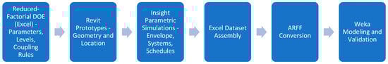
Figure 1.
BIM-ML data integration workflow illustrating the six-stage pipeline used in this study: (1) reduced-factorial DOE construction in Excel with parameter levels and coupling rules; (2) geometric and locational prototype modeling in Revit; (3) parametric energy simulations executed in Insight; (4) simulation output assembly and structuring in Excel; (5) ARFF file preparation for ML compatibility; and (6) model training, validation, and feature-importance analysis in Weka.
Both coupling constraints—namely (i) HVAC-orientation applicability and (ii) façade WWR coordination through predefined glazing patterns—were enforced directly within the reduced-factorial scheduling rules defined in Section 2.3, ensuring physically realistic system-orientation combinations, controlled façade parametrization, and full repeatability across the BIM-ML pipeline.
3. Results
This section presents the outcomes of the ML analysis developed to predict building energy performance based on the dataset generated from Revit-Insight simulations. The results are organized to describe the predictive accuracy of the trained models, compare the performance of the four algorithms, and interpret the influence of design and operational parameters on the two dependent indicators: EUI (kBtu/ft2·yr) and OE (kBtu/yr).
3.1. Model Training and Predictive Performance
Four regression algorithms—LR, M5P, SMOReg (with polynomial and radial basis function kernels), and RF—were evaluated using 10-fold cross-validation. Model accuracy was measured through the R2, RMSE, and MAE.
Table 2 summarizes the comparative performance of the ML algorithms used. All algorithms demonstrated strong predictive capability for both EUI and OE, achieving R2 values above 0.95. Among them, the RF model provided the highest overall accuracy, with R2 = 0.977 for EUI and R2 = 0.974 for OE, along with lower RMSE (6.57 kBtu/ft2·yr and 4.10 × 10⁶ kBtu/yr) and MAE (2.81 kBtu/ft2·yr and 1.75 × 10⁶ kBtu/yr). The LR and SMOReg (Polynomial) models also achieved competitive results, confirming that both linear and kernel-based methods effectively captured relationships among BIM-derived variables.
Table 2.
Comparative performance of ML algorithms for energy prediction.
These findings indicate that the ML algorithms successfully modeled the nonlinear interactions between geometric, envelope, system, and operational parameters. The RF model exhibited the best balance between accuracy and robustness, with minimal error dispersion across model types.
The scatterplots of predicted versus simulated values (Figure 2 and Figure 3) show a near-linear alignment along the 1:1 diagonal, demonstrating that the models, particularly RF, accurately replicated the simulation trends and achieved unbiased predictions across the energy range.
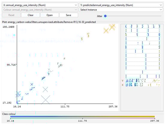
Figure 2.
Predicted versus simulated EUI values for the RF model. Derived from BIM-ML results in Weka.
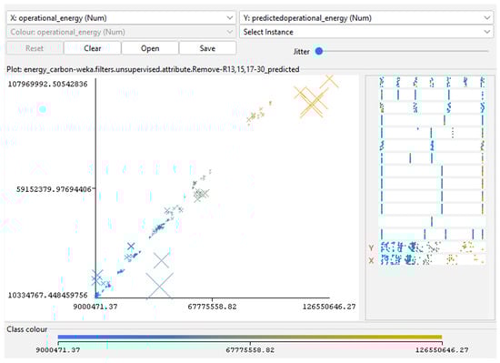
Figure 3.
Predicted versus simulated OE values for the RF model. Derived from BIM-ML model results in Weka.
Beyond numerical accuracy, the results highlight the practical applicability of the trained surrogate models for early design decision-making. The near-linear correspondence between simulated and predicted outcomes suggests that the ML models can reliably approximate simulation-based results with substantially reduced computation time. Such consistency reinforces the potential of the BIM-ML workflow to function as a rapid screening tool for design alternatives, supporting sensitivity analysis and guiding parameter prioritization prior to detailed energy modeling. This capability is particularly valuable for iterative concept development, where timely performance feedback can significantly improve energy-conscious architectural decisions.
3.2. Feature Importance Analysis
Feature importance was evaluated using the ClassifierAttributeEval method combined with the Ranker approach in Weka, employing RF as the base learner. This analysis quantified the relative contribution of each independent variable to EUI and OE prediction.
As summarized in Table 3, HVAC system type, WWR, and operation schedule emerged as the most influential predictors of building energy performance. Plug loads and infiltration rate followed as secondary variables, reflecting their role in internal heat gains and air exchange. Orientation exhibited moderate influence, confirming the impact of façade alignment on solar exposure and envelope performance. In contrast, geometric descriptors such as shape and GFA contributed minimally, indicating that system-level and operational variables outweighed form-based variations in the warm-humid context of ASHRAE Climate Zone 2A [27].
Table 3.
Feature importance ranking for EUI and OE prediction based on the RF model.
When the 168-model baseline was expanded to the 210-model dataset, sensitivity patterns remained consistent, though the magnitude of influence increased for HVAC, WWR, and schedule variables. This shift suggests that as model diversity improved, the RF surrogate model converged toward stronger dependence on system-driven and envelope-related parameters, reinforcing the importance of efficiency and façade configuration in energy-performance prediction.
The results collectively confirm that energy consumption in hot-humid climates is primarily governed by:
- HVAC performance (system efficiency);
- Façade composition (glazing ratios and orientation); and
- Occupant-driven operation schedules.
These findings align with the observed feature-importance scores illustrated in Figure 4, which compare EUI and OE results across the 168 and 210-model datasets.
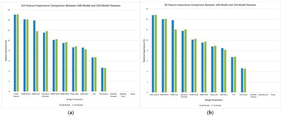
Figure 4.
Comparison of feature-importance scores for EUI and OE prediction between the 168-model baseline dataset and the expanded 210-model dataset: (a) EUI feature-importance comparison; (b) OE feature-importance comparison. The 168-model dataset refers to the reduced-factorial baseline DOE, while the 210-model dataset includes the baseline plus 32 generalization and 10 stress-test models. Bars represent normalized relative importance scores derived from the RF model in Weka.
4. Discussion
The integration of BIM-based simulation data with ML regression techniques proved highly effective for predicting building energy performance during the conceptual design phase. Among the four algorithms tested, the RF model overall outperformed the others under default parameter settings, achieving high predictive accuracy (R2 > 0.97) and low error rates. The consistently high R2 values observed across all models reflect the strong deterministic physical relationships inherent to building energy performance under a structured parametric design, rather than data overfitting, as confirmed by cross-validation, generalization testing, and stress-testing. These findings are consistent with previous studies demonstrating that ensemble learning algorithms can deliver robust and generalizable predictions for building energy analysis while reducing computational demand compared to physics-based simulations [9,10].
The feature-importance analysis further revealed that system, envelope, and operational parameters, particularly HVAC system type, WWR, and operation schedule, were the dominant factors influencing energy performance. This result aligns with prior research identifying mechanical system efficiency, envelope, and occupancy control as key drivers of operational energy consumption, surpassing the influence of geometric characteristics such as building shape and orientation [32]. In warm-humid climates such as Orlando (ASHRAE Climate Zone 2A) [27], earlier investigations similarly found that façade transparency and HVAC performance have a compounded effect on cooling loads and overall energy use [33].
The strong agreement between predicted and simulated results demonstrates that ML-based surrogate models can replicate energy simulation outcomes with minimal deviation. By integrating Revit, Insight, and Weka within a unified workflow, this study bridges the gap between simulation-based and data-driven evaluations, offering an interpretable and repeatable framework for early-stage performance prediction. This integration enables design teams to estimate energy implications rapidly, prioritize impactful parameters, and make more informed design decisions before proceeding to detailed analysis.
Overall, these results corroborate emerging research advocating BIM-ML integration as a practical and transparent approach to early-stage sustainability assessment [19]. The proposed framework advances energy modeling by combining predictive accuracy with interpretability, promoting data-driven design practices that support the creation of energy-efficient and environmentally responsible buildings.
All reported predictive performances reflect algorithm behavior under default parameter settings, as no hyperparameter tuning was performed in this study. This modeling choice was intentional and aligned with the primary objective of evaluating the intrinsic predictive capability and generalization behavior of different algorithms on a statistically balanced DOE-generated dataset, rather than maximizing performance through data-dependent optimization. Accordingly, the superior performance observed for the RF model should be interpreted strictly as performance under default settings, ensuring methodological transparency and preventing over-interpretation of algorithm optimality.
Dataset Sufficiency and Overfitting Control
While the dataset size (N = 210) may appear modest relative to the number of input parameters, the reduced-factorial DOE [25,26] was purposefully constructed to ensure statistically rigorous and non-redundant coverage of the design space, effectively mitigating collinearity and sampling bias inherent to random designs. The consistently strong predictive performance observed across baseline, expanded, and stress-test scenarios demonstrates that the models are learning the governing physical relationships embedded in building energy simulations, rather than overfitting to the available samples. Furthermore, the intentional omission of hyperparameter tuning enforces conservative model behavior, prioritizing robustness and generalizability over performance-driven optimization.
5. Conclusions
This study developed and validated a BIM-based ML framework for predicting the energy performance of office buildings during early design stages. By integrating Revit and Insight simulations with Weka-based regression analysis, the workflow provided an automated, transparent, and reproducible process for assessing EUI and OE using design and operational parameters.
Among the four algorithms tested—LR, M5P, SMOReg, and RF—the RF model achieved the best predictive performance overall under default parameter settings, with R2 values exceeding 0.97 and mean errors below 5%. Feature importance analysis identified HVAC system type, WWR, and operation schedule as the most influential variables affecting energy outcomes. These findings emphasize the strong impact of system, envelope and operational choices compared to geometric characteristics during the conceptual design phase.
The results confirm that ML-based surrogate modeling can effectively replicate simulation outcomes and provide rapid feedback without the need for additional energy runs. The proposed BIM-ML framework thus supports early decision-making by enabling architects and engineers to evaluate multiple design scenarios quickly and objectively, improving energy efficiency outcomes while reducing modeling complexity.
From an engineering practice perspective, the proposed BIM-ML framework enables rapid screening of alternative early-stage design solutions without the need for repeated energy simulations. Designers can directly evaluate the energy implications of multi-parameter design decisions, including building geometry, orientation, envelope properties, glazing ratios, HVAC system selection, infiltration levels, lighting and plug load densities, and operational schedules, with near-simulation accuracy, substantially reducing decision-making time during conceptual design. This allows project teams to identify high-impact performance drivers early, optimize system selection, and reduce downstream rework. The framework is therefore directly applicable to feasibility studies, sustainability-driven design iterations, and performance-based design workflows in professional practice.
Despite the strong predictive performance and practical applicability of the proposed framework, several limitations should be acknowledged to properly define the scope and transferability of the present findings.
5.1. Limitations and Scope of Applicability
This study is limited to office-building prototypes located in Orland, Florida (ASHRAE Climate Zone 2A [27]), and therefore primarily reflects cooling-dominated energy behavior characteristic of warm-humid climates. The trained surrogate models may not be directly transferable to cold or arid climates without retraining using region-specific datasets. Additionally, simulations relied on typical meteorological year (TMY) weather files automatically assigned by the Insight engine for the selected project location and did not incorporate real-time weather variability or measured operational data. The dataset represents a controlled parametric design space rather than an uncontrolled real-world building operation. Addressing these limitations would require multi-climate dataset expansion, integration of measured building performance data, and comparative benchmarking against other BIM-ML platforms.
External validation using measured building performance data was intentionally excluded from the present study, as the primary objective was to rigorously assess surrogate-model learning behavior under controlled, reproducible simulation conditions where ground-truth relationships are explicitly defined. Introducing empirical datasets at this stage would confound the interpretation of model behavior due to measurement noise, operational variability, and undocumented control strategies that are extraneous to the methodological contribution of this work. Validation across multiple climates and against real-world building performance using independent datasets is, therefore, a logical and necessary extension of the proposed framework and is explicitly identified as a direction for future research.
5.2. Future Research Directions
Future research should extend this approach to multi-climate datasets and integrate embodied carbon and lifecycle metrics to create a unified predictive framework for total building performance assessment. Expanding the dataset with real-world building data and incorporating physics-informed or hybrid modeling techniques may further enhance prediction accuracy and broaden the applicability of the proposed framework across diverse building typologies and design contexts.
Future studies should also include systematic cross-platform benchmarking of the proposed framework against alternative ML environments (e.g., Python-based platforms such as Scikit-Learn and TensorFlow) to further quantify algorithmic consistency, robustness, and computational scalability.
Future work should also focus on validating the proposed framework using independent external datasets derived from measured building performance and alternative simulation environments, to formally quantify out-of-sample generalization and transferability.
Author Contributions
Conceptualization, L.M.d.P., A.O., and O.T.; methodology, L.M.d.P.; software, L.M.d.P.; validation, L.M.d.P.; formal analysis, L.M.d.P.; investigation, L.M.d.P.; resources, L.M.d.P.; data curation, L.M.d.P.; writing—original draft preparation, L.M.d.P.; writing—review and editing, A.O. and O.T.; visualization, L.M.d.P.; supervision, A.O. and O.T. All authors have read and agreed to the published version of the manuscript.
Funding
This research received no external funding.
Institutional Review Board Statement
Not applicable.
Informed Consent Statement
Not applicable.
Data Availability Statement
The dataset supporting this study is openly available at Zenodo, titled “BIM-Based Dataset for ML Energy Prediction.” All data used for model training and validation can be downloaded at: https://doi.org/10.5281/zenodo.17417879 (accessed on 22 October 2025), Excel File: BIM-Based Dataset for Energy Prediction.xlsx, Attribute-Relation File Format: relation final_eui_regressor.arff and relation final_oe_regressor.arff.
Acknowledgments
The authors thank the University of Central Florida for providing the academic environment that supported this research.
Conflicts of Interest
The authors declare no conflict of interest.
Abbreviations
The following abbreviations are used in this manuscript:
| ANN | Artificial Neural Network |
| ARFF | Attribute-Relation File Format |
| ASHRAE | American Society of Heating, Refrigerating and Air-Conditioning Engineers |
| BIM | Building Information Modeling |
| BPS | Building Performance Simulation |
| CO2 | Carbon Dioxide |
| DOE | Design of Experiments |
| DOE-2 | Department of Energy-2 |
| EUI | Energy Use Intensity |
| GFA | Gloss Floor Area |
| GSHP with DOAS + ERV | Ground Source Heat Pump system with Dedicated Outdoor Air System and Energy Recovery Ventilation |
| HVAC | Heating, Ventilation, and Air Conditioning |
| LPD | Lighting Power Density |
| LR | Linear Regression |
| M5P | Model Tree |
| MAE | Mean Absolute Error |
| ML | Machine Learning |
| OE | Operational Energy |
| R2 | Coefficient of Determination |
| RBF | Radial Basis Function |
| RF | Random Forest |
| RMSE | Root Mean Square Error |
| SMOReg | Sequential Minimal Optimization Regression |
| SVM | Support Vector Machine |
| TMY | Typical Meteorological Year |
| VAV w/WC and EB | Variable Air Volume system with Water-Cooled chiller and Electric Boiler |
| VAV w/WC and GAS | Variable Air Volume system with Water-Cooled chiller and Gas Boiler |
| WWR | Window-to-Wall Ratio |
Appendix A
Appendix A.1. Experimental Matrix Construction
This appendix documents the step-by-step method used to construct the reduced-factorial dataset that guided the Revit-Insight simulations. All procedures were executed in Microsoft Excel to ensure transparency, traceability, and reproducibility.
Appendix A.1.1. Definition of Parameters and Levels
Eleven independent design parameters were listed in separate Excel columns as defined in Table 1 of the main text: shape, orientation, HVAC system, infiltration rate, LPD, operation schedule, plug loads, and WWR for each façade (North, East, South, West).
Each column contained only the predefined levels selected for the reduced-factorial design. For example:
- Orientation: {0°, 45°, 90°, 180°}
- HVAC: {Base by Design, VAV w/WC and Gas, VAV w/WC and EB, GSHP w/DOAS + ERV}
- Infiltration: {0.04, 0.09, 0.12 CFM/ft2}
Appendix A.1.2. Shape Area Mapping
Each geometric type was linked to its GFA using a static lookup Table A1.
Table A1.
Shape area mapping is used in the reduced-factorial design.
Table A1.
Shape area mapping is used in the reduced-factorial design.
| Shape | GFA (ft2) |
|---|---|
| Square | 30,401 |
| Rectangular | 30,411 |
| Cross | 29,421 |
| T | 27,061 |
| H | 28,641 |
| U | 29,421 |
| L | 30,744 |
Based on Revit model bounding box measurements.
The GFA column was automatically populated using the VLOOKUP function referencing this table.
Appendix A.1.3. Initial Combination Assembly
Feasible combinations were expanded using Excel’s Fill Down, INDEX, and CONCATENATE functions to produce an initial list of candidate configurations across the 11 columns.
This list represented the unfiltered factorial space prior to the application of coupling rules and pruning.
Appendix A.1.4. Coupling and Filtering Rules
- 1.
- HVAC-orientation coupling
To ensure realistic system-orientation pairs, only six combinations were retained:
(1) Base by Design-0°, (2) Base by Design-45°, (3) GSHP w/DOAS + ERV-0°, (4) GSHP w/DOAS + ERV-45°, (5) VAV w/WC and Gas-90°, (6) VAV w/WC and EB-180°.
Invalid pairs were filtered using IF and MATCH formulas, with non-compliant rows flagged and excluded.
- 2.
- WWR pattern coordination
Façade glazing ratios were constrained to nine curated patterns representing architecturally coherent distributions of WWRs:
[0, 0, 0, 0], [0, 0, 0, 30], [0, 0, 50, 50], [0, 30, 0, 0], [30, 0, 30, 30], [30, 30, 30, 0], [30, 30, 30, 30], [50, 50, 0, 0], [50, 50, 50, 50].
Patterns outside these combinations were automatically excluded.
- 3.
- Manual balancing and selection
From the filtered combinations, 168 unique configurations were manually selected to achieve near-uniform level representation and approximate orthogonality.
Level frequencies were monitored using COUNTIFS and summarized through PivotTables until deviations from ideal counts remained within ±12 runs per level.
No configuration was duplicated.
Each valid configuration received a sequential model ID (M-001–M-168) using the Fill Series function.
This reduced-factorial dataset formed the base matrix for the simulations.
- 4.
- Dataset expansion
To broaden parameter coverage, 32 generalization models (M-169–M-200) were later appended to improve representation of under-sampled combinations while preserving coupling constraints and façade-pattern rules.
For model robustness assessment, 10 stress-test cases (M-201–M-210) were manually added:
- High-load group: LPD = 1.00 W/ft2, plug load = 1.3 W/ft2, infiltration rate = 0.12 CFM/ft2, 24/7 operation schedule, high-glazing façades ([50, 50, 50, 50]/[50, 50, 0, 0]).
- Low-load group: LPD = 0.45 W/ft2, plug load = 1.0 W/ft2, infiltration rate = 0.04 CFM/ft2, 8 a.m.–5 p.m. operation schedule, low-glazing façades, GSHP w/DOAS + ERV systems.
All stress-test and generalization models adhered to the same shape-area mapping and parameter dependencies as the base design.
- 5.
- Validation and diagnostics
Level balance diagnostics compared actual versus ideal level frequencies (ideal = N/L, where N = 168 and L represents the number of levels defined for each parameter in Table 1 of the main text).
Deviations across all parameters remained within ±12 runs per level, confirming satisfactory statistical balance and approximate orthogonality consistent with DOE best practices.
The verified Excel matrix served as the master control file for generating Revit building prototypes and corresponding Insight simulations.
Appendix A.1.5. Replication Notes
- Software: Autodesk Revit 2024 + Insight Carbon Analysis 2023.1; Microsoft Excel 2024; Weka 3.8.6.
- Location and weather: Orlando, Florida (ASHRAE Climate Zone 2A) [27].
- Simulation consistency: identical project location, floor heights, and baseline geometry across all prototypes.
Appendix A.1.6. Summary
This protocol provides the full procedural transparency required to reproduce the 210-model dataset used in this study.
By combining structured parameterization, manual level balancing, and controlled boundary testing, the Excel-based DOE framework ensures reproducibility and methodological rigor in data-driven building performance research.
Appendix B
Dataset Attributes and Structure of the ARFF Files
This appendix supports the reproducibility of the BIM-ML framework by detailing the structure and attributes of the dataset used for ML analysis in Table A2.
All variables were derived from Insight simulations linked to Revit-generated models and compiled into an ARFF in Notepad for use in Weka.
The dataset includes both categorical and numerical parameters representing geometric, envelope, system, and operational characteristics of the modeled office buildings. Two dependent variables—EUI and OE—served as the predictive targets for model training and evaluation.
Table A2.
Dataset attributes included in the ARFF file used for ML modeling.
Table A2.
Dataset attributes included in the ARFF file used for ML modeling.
| Parameter | Type | Range |
|---|---|---|
| Shape | Categorical | Square, Rectangular, Cross, L, U, H, and T |
| Orientation (°) | Numeric | 0, 45, 90, 180 |
| HVAC System | Categorical | Base by Design, VAV w/WC and Gas, VAV w/WC and EB, GSHP w/DOAS + ERV |
| Infiltration (CFM/ft2) | Numeric | 0.04, 0.09, 0.12 |
| Lighting Power Density (W/ft2) | Numeric | 0.45, 0.72, 1.00 |
| Operation Schedule | Categorical | 8 a.m.–5 p.m., 12/5, 24/7 |
| Plug Loads (W/ft2) | Numeric | 1.0, 1.3 |
| WWR East (%) | Numeric | 0, 30, 50 |
| WWR North (%) | Numeric | 0, 30, 50 |
| WWR South (%) | Numeric | 0, 30, 50 |
| WWR West (%) | Numeric | 0, 30, 50 |
| Building Lifespan (years) | Numeric | Fixed (20) |
| Emissions Factor (kg CO2e/ft2.y) | Numeric | Fixed (0.45) |
| Gross Floor Area (ft2) | Numeric | ≈27,000–31,000 |
| Dependent Variable 1: EUI (kBtu/ft2.yr) | Numeric | 17–180 |
| Dependent Variable 2: OE (kBtu/year) | Numeric | 1.8 × 10⁶–12.0 × 10⁶ |
Note: EUI and OE values were derived from BIM-ML model results in Weka. The emission factor (0.45 kg CO2e/kWh) was a fixed constant defined within Insight simulations and therefore was not included as a variable in the ARFF dataset. Building lifespan was kept constant across all simulations, and the gross floor area was maintained within a narrow range to ensure geometric comparability.
References
- Ritchie, H.; Rosado, P. Energy Mix; Our World in Data. January 2024. Available online: https://ourworldindata.org/energy-mix (accessed on 20 October 2025).
- U.S. Energy Information Administration (EIA). Electricity Explained. 2023. Available online: https://www.eia.gov/energyexplained/electricity/electricity-in-the-us.php (accessed on 20 October 2025).
- United Nations Environment Programme; International Energy Agency (IEA). Global Status Report for Buildings and Construction 2024; UN Environment Programme: Nairobi, Kenya, 2024; Available online: https://globalabc.org/resources/publications/global-status-report-buildings-and-construction-20242025-not-just-another (accessed on 20 October 2025).
- Harish, V.S.K.V.; Kumar, A. A review on modeling and simulation of building energy systems. Renew. Sustain. Energy Rev. 2016, 56, 1272–1292. [Google Scholar] [CrossRef]
- Seyedzadeh, S.; Ramezani, P.F.; Glesk, I.; Roper, M. Machine learning for estimation of building energy consumption and performance: A review. Vis. Eng. 2018, 6, 5. [Google Scholar] [CrossRef]
- Fumo, N.; Biswas, M.A.R. Regression analysis for prediction of residential energy consumption. Renew. Sustain. Energy Rev. 2015, 47, 332–343. [Google Scholar] [CrossRef]
- Kalogirou, S.A. Applications of artificial neural networks in energy systems: A review. Energy Convers. Manag. 1999, 40, 1073–1087. [Google Scholar] [CrossRef]
- Ahmad, A.S.; Hassan, M.Y.; Abdullah, H.; Rahman, H.A.; Hussin, F.; Abdullah, M.P.; Said, D.M. A review on applications of ANN and SVM for building electrical energy consumption forecasting. Renew. Sustain. Energy Rev. 2018, 33, 102–109. [Google Scholar] [CrossRef]
- Duarte, G.R.; Fonseca, L.G.; Goliatt, P.V.Z.C.; Lemonge, A.C.C. Comparison of machine learning techniques for predicting energy loads in buildings. Ambient Constr. 2017, 17, 3. [Google Scholar]
- Wang, Z.; Wang, Y.; Zeng, R.; Srinivasan, R.S.; Ahrentzen, S. Random Forest based hourly building energy prediction. Energy Build. 2018, 171, 11–25. [Google Scholar] [CrossRef]
- Walker, S.; Khan, W.; Katic, K.; Maassen, W.; Zeiler, W. Accuracy of different machine learning algorithms and added-value of predicting aggregated-level energy performance of commercial buildings. Energy Build. 2020, 209, 109705. [Google Scholar] [CrossRef]
- Robinson, C.; Dilkina, B.; Hubbs, J.; Zhang, W.; Guhathakurta, S.; Brown, M.A.; Pendyala, R.M. Machine learning approaches for estimating commercial building energy consumption. Appl. Energy 2017, 208, 889–904. [Google Scholar] [CrossRef]
- Amasyali, K.; El-Gohary, N.M. A review of data-driven building energy consumption prediction studies. Renew. Sustain. Energy Rev. 2018, 81, 1192–1205. [Google Scholar] [CrossRef]
- Gao, T.; Han, X.; Wang, J.; Geng, Y.; Zhang, H.; Song, T. Enhancing building energy efficiency: An integrated approach to predicting heating and cooling loads using machine learning and optimization algorithms. J. Build. Eng. 2024, 98, 110759. [Google Scholar] [CrossRef]
- Bouathri, Y.; Tilioua, A. Machine learning-based predictive model for thermal comfort and energy optimization in smart buildings. Results Eng. 2024, 22, 102148. [Google Scholar] [CrossRef]
- Lu, Y.; Wu, Z.; Chang, R.; Li, Y. Building Information Modeling (BIM) for green buildings: A critical review and future directions. Autom. Constr. 2017, 83, 134–148. [Google Scholar] [CrossRef]
- Ma, G.; Liu, Y.; Shang, S. A building information model (BIM) and artificial neural network (ANN) based system for personal thermal comfort evaluation and energy efficient design of interior space. Sustainability 2019, 11, 4972. [Google Scholar] [CrossRef]
- Pan, X.; Khan, A.M.; Eldin, S.M.; Aslam, F.; Rehman, S.K.U.; Jameel, M. BIM adoption in sustainability, energy modelling and implementing using ISO 19650: A review. Ain Shams Eng. J. 2024, 15, 102252. [Google Scholar] [CrossRef]
- Khan, A.A.; Khan, M.A.; Ahmad, N.; Jamil, F.; Imran, M.; Abaker, M. Integrating Building Information Modelling and artificial intelligence: A systematic review of challenges and mitigation strategies. Technologies 2024, 12, 185. [Google Scholar] [CrossRef]
- Hollberg, A.; Genova, G.; Habert, G. Evaluation of BIM-based LCA results for building design. Autom. Constr. 2020, 109, 102972. [Google Scholar] [CrossRef]
- Ning, C.; You, F. Optimization under uncertainty in the era of big data and deep learning: When machine learning meets mathematical programming. Comput. Chem. Eng. 2019, 125, 434–448. [Google Scholar] [CrossRef]
- Feng, K.; Lu, W.; Wang, Y. Assessing environmental performance in early building design stage: An integrated parametric design and machine learning method. Sustain. Cities Soc. 2019, 50, 101596. [Google Scholar] [CrossRef]
- D’Amico, B.; Myers, R.J.; Sykes, J.; Voss, E.; Cousins-Jenvey, B.; Fawcett, W.; Richardson, S.; Kermani, A.; Pomponi, F. Machine learning for sustainable structures: A call for data. Structures 2019, 19, 1–4. [Google Scholar] [CrossRef]
- Hong, T.; Luo, X.; Zhang, W. Ten questions on data-driven building performance modeling. Build. Environ. 2020, 168, 106508. [Google Scholar] [CrossRef]
- Box, G.E.P.; Hunter, J.S.; Hunter, W.G. Statistics for Experimenters: Design, Innovation, and Discovery, 2nd ed.; John Wiley & Sons: Hoboken, NJ, USA, 2005. [Google Scholar]
- Montgomery, D.C. Design and Analysis of Experiments, 9th ed.; John Wiley & Sons: Hoboken, NJ, USA, 2017. [Google Scholar]
- ASHRAE. ANSI/ASHRAE/IES Standard 90.1-2019: Energy Standard for Buildings Except Low-Rise Residential Buildings; American Society of Heating, Refrigerating and Air-Conditioning Engineers: Atlanta, GA, USA, 2019. [Google Scholar]
- Atkinson, A.C.; Donev, A.N.; Tobias, R.D. Optimum Experimental Designs, with SAS; Oxford University Press: Oxford, UK, 2007. [Google Scholar]
- Shahriari, B.; Swersky, K.; Wang, Z.; Adams, R.P.; de Freitas, N. Taking the Human Out of the Loop: A Review of Bayesian Optimization. Proc. IEEE 2016, 104, 148–175. [Google Scholar] [CrossRef]
- Lawrence Berkeley National Laboratory (LBNL). DOE-2: Building Energy Use and Cost Analysis Tool. Available online: https://doe2.com/DOE2 (accessed on 20 October 2025).
- U.S. Department of Energy (DOE). Energyplus: Building Energy Simulation Program. Available online: https://energyplus.net (accessed on 20 October 2025).
- Khan, A.M.; Tariq, M.A.; Rehman, S.K.U.; Saeed, T.; Alqahtani, F.K.; Sherif, M. BIM Integration with XAI Using LIME and MOO for Automated Green Building Energy Performance Analysis. Energies 2024, 17, 3295. [Google Scholar] [CrossRef]
- Rahmani Asl, M.; Xu, W.; Shang, J.; Tsai, B.; Molloy, I. Regression-Based Building Energy Performance Assessment Using Building Information Model (BIM). In Proceedings of the ASHRAE and IBPSA-USA SimBuild 2016 Building Performance Modeling Conference, Salt Lake City, UT, USA, 8–12 August 2016. [Google Scholar]
Disclaimer/Publisher’s Note: The statements, opinions and data contained in all publications are solely those of the individual author(s) and contributor(s) and not of MDPI and/or the editor(s). MDPI and/or the editor(s) disclaim responsibility for any injury to people or property resulting from any ideas, methods, instructions or products referred to in the content. |
© 2025 by the authors. Licensee MDPI, Basel, Switzerland. This article is an open access article distributed under the terms and conditions of the Creative Commons Attribution (CC BY) license.