EGA: An Efficient GPU Accelerated Groupby Aggregation Algorithm

Abstract

With the exponential growth of big data, efficient groupby aggregation (GA) has become critical for real-time analytics across industries. GA is a key method for extracting valuable information. Current CPU-based solutions (such as large-scale parallel processing platforms) face computational throughput limitations. Since CPU-based platforms struggle to support real-time big data analysis, the GPU is introduced to support real-time GA analysis. Most GPU GA algorithms are based on hashing methods, and these algorithms experience performance degradation when the load factor of the hash table is too high or when the data volume exceeds the GPU memory capacity limit. This paper proposes an efficient hash-based GPU-accelerated groupby aggregation algorithm (EGA) that addresses these limitations. EGA features different designs for different scenarios: single-pass EGA (SP-EGA) maintains high efficiency when data fit in the GPU memory, while multipass EGA (MP-EGA) supports GA for data exceeding the GPU memory capacity. EGA demonstrates significant acceleration: SP-EGA outperforms SOTA hash-based GPU algorithms by 1.16–5.39× at load factors >0.90 and surpasses SOTA sort-based GPU methods by 1.30–2.48×. MP-EGA achieves 6.45–29.12× speedup over SOTA CPU implementations.

1. Introduction

With the rapid development of information technology, the generation and application of big data have become significant characteristics of contemporary society. Traditional data processing methods, especially in distributed environments, struggle with data’s rapid growth and diversification. The efficient analysis of massive datasets remains a critical research challenge [1]. In this context, Group By Aggregation (GA) has demonstrated considerable for application potential in the field of large-scale data analysis. GA is primarily utilized to extract valuable information from vast datasets; by grouping and aggregating data, GA enables organizations to identify trends, optimize decision-making, and enhance efficiency. This method proves essential for log analysis, social media, finance, and healthcare applications [2,3,4,5].

Currently, many big data processing tasks rely on Massively Parallel Processing (MPP) platforms, such as Dremel, Apache Spark (v3.4.4), and Redshift (v3.5.11) [6,7]. These platforms achieve efficient data processing by distributing computational tasks across multiple computing nodes. However, existing MPP platforms exhibit several notable characteristics in practical applications. First, the low density of computing cores results in insufficient computational throughput, making it difficult to meet the demands of real-time data processing. Second, the dispersed storage of data significantly increases the overhead of data exchange, thereby reducing the overall performance of the system. Furthermore, many computational tasks often undergo multiple stages, akin to the Map/Reduce computation process, which adds latency and affects the ability to perform real-time computations.

When dealing with operators that require substantial computational resources such as GA, achieving near-real-time computation becomes challenging. To address this challenge, the application of Graphics Processing Units (GPUs) in the field of big data analysis has garnered increasing attention [8,9,10]. For instance, platforms like Apache Spark and NVIDIA RAPIDS (v25.02) leverage the GPU acceleration for data analysis, significantly enhancing computational efficiency. Apache Spark supports the allocation of computational tasks to GPUs, thereby accelerating data processing and machine learning tasks, while NVIDIA RAPIDS provides a comprehensive suite of GPU-accelerated libraries that optimize data science and analytical workflows.

GPUs have been widely used in the acceleration of GA. Existing GPU GA algorithms are either hash-based or sort-based. Some previous studies have shown that hash-based GA methods are superior to sort-based GA methods [11]. However, existing hash-based GA algorithms that utilize GPU acceleration exhibit certain limitations [1,12]. Hash-based algorithms require a hash table. In the following two scenarios, hash-based algorithms will face performance degradation: first, when the load factor of hash table is excessively high, the computational efficiency of the platform significantly declines, failing to fully exploit the advantages of GPUs; second, when the data volume exceeds the GPU’s memory capacity, there are no platforms available that can make full use of the GPU for GA acceleration.

To address the aforementioned challenges, this paper proposes EGA, an efficient GPUaccelerated groupby aggregation algorithm. In this paper, our main contributions are as follows: In the situation that data could fit in GPU memory, single-pass EGA (SP-EGA) is designed to maintain high computational efficiency even when the load factor of the hash table is 1.0. SP-EGA achieves acceleration factors ranging from 1.16 to 5.39 times compared to the state-of-the-art (SOTA) hash-based GA algorithm on the GPU when the load factor exceeds 0.90 and achieves acceleration factors ranging from 1.30 to 2.48 times compared to the SOTA sort-based GA algorithm on the GPU. In situations where data could not fit in GPU memory, multi-pass EGA (MP-EGA) is designed to support data GA that exceeds GPU memory capacity. MP-EGA still achieves acceleration factors of 6.45 to 29.12 times compared to SOTA algorithms on a CPU. This innovative method provides a new solution for large-scale data analysis.

2. Related Work

Early work investigated multi-core CPUs for groupby acceleration. Müller et al. observed that, in multi-core CPU architectures, groupby operations using hash-based methods and sorting-based methods share significant similarities [13]. Cieslewicz et al. proposed several parameter recommendations for data structures to optimize groupby operations in multi-core CPU environments [14].

In recent years, with the rapid development of GPU technology, researchers have increasingly focused on implementing groupby operations on GPUs. Research on GPU acceleration algorithms for GA can be mainly divided into the following two categories: hash-based methods and sorting-based methods.

In the sorting-based approach, He et al. were among the first to utilize GPU-based sorting to enhance groupby aggregation algorithms [15]. Additionally, Bakkum et al. implemented a sorting-based groupby aggregation in SQLite, showcasing its effectiveness in database operations [16]. Do et al. proposed a sorting algorithm with adaptive capabilities that integrates the advantages of traditional sorting and hashing algorithms, eliminating the need for users to select different algorithms based on conditions such as data size and data distribution characteristics [17]. Bala et al. found that current sorting solutions cannot fully utilize modern GPUs’ parallel processing capabilities due to the need for synchronizing threads accessing shared memory [18]. To address this, they propose a novel method to reduce the overhead of accessing aggregate memory locations through atomic operations.

The advantage of sorting-based methods is that their performance is relatively stable and can maintain good performance across various data group sizes. However, previous research has indicated that hash-based methods outperform sorting-based methods when the data group size is medium or small [1]. Therefore, in order to achieve better performance when the number of data groups is moderate or small, there are also studies on hash-based data grouping and aggregation algorithms.

In the hash-based approach, Amenta et al. implemented a set of parallel hash table techniques, including open addressing, chaining, and cuckoo hashing, and evaluated their performance in terms of memory usage, construction time, and retrieval efficiency under different scenarios [19]. This study preliminarily confirms the possibility of accelerating hashing with GPUs, but it has not yet been applied to data analysis applications such as group aggregation of data. Karnagel et al. proposed a hash table-based groupby aggregation algorithm that employs linear probing to resolve conflicts [1]. However, they noted that the hash table design must align with the constraints of the GPU global memory (GM), with a recommended load factor of approximately 0.5. That is to say, in this study, half of the hash table will be empty, which will result in significant space wastage. Tome et al. proposed using hash tables of different granularities in different scenarios: when the data volume is small, the hash table can be placed in shared memory or even registers; when the data volume is large, the hash table can be placed in global memory. However, this division requires the ability to estimate the number of data groups in advance to determine whether to place the hash table in faster storage (such as GPU L2 or shared memory), thus limiting the applicability of this method. Rosenfeld et al. systematically analyzed the impact of GPU architectures (covering four NVIDIA generations and two AMD GCN) on hash aggregation performance, revealing that hardware dependency fundamentally limits the generalizability of prior heuristic methods (NVIDIA Corporation, Santa Clara, CA, USA; Advanced Micro Devices, Inc., Santa Clara, CA, USA). They proposed a dynamic tuning algorithm leveraging the convexity of configuration space, achieving less than 1% performance loss in 90% cases within 1% of full search time, establishing a new paradigm for operator optimization in heterogeneous computing [20]. However, this method is highly dependent on hardware, requiring the search for corresponding optimal parameters for each type of hardware, which limits the widespread use of this approach.

The above studies were conducted under the assumption that the data could be fully loaded into GPU memory. We found that these methods perform excellently in specific scenarios, but none of them can maintain excellent performance in general scenarios. For example, the sorting-based GPU-accelerated data grouping and aggregation algorithm perform poorly when the number of data groups is moderate or small, while the hash-based GPU-accelerated grouping and aggregation algorithm generally requires that the load factor of the hash table should not be too large, typically recommended not to exceed 0.5, which leads to significant space waste. Therefore, our research aims to find a GPU-accelerated data grouping and aggregation algorithm that maintains ultra-high performance in general scenarios. Our work has chosen the hash-based acceleration direction, so we attempt to overcome a major drawback of current hash-based GPU-accelerated data grouping and aggregation algorithms: the space waste in GPU memory caused by the load factor of the hash table not being too large.

The above research assumes that the data can be fully accommodated in GPU memory. So, what happens when the size of the data exceeds the GPU memory capacity? Consequently, there has been some research on data grouping and aggregation algorithms based on CPU–GPU heterogeneous computing systems. For instance, Abdelhafeez et al. proposed a distributed query architecture that utilizes a global distributed spatial index to construct partitions, thereby accelerating groupby operations [21]. Similarly, Diego et al. improved the performance of CPU–GPU heterogeneous systems by employing parallelism-friendly compression techniques and efficient scheduling strategies, demonstrating superior performance compared to single-system implementations in groupby tasks [20].

However, the performance of GPU–CPU heterogeneous systems is often constrained by the bandwidth limitations of the PCIe bus connecting GPUs and CPUs [22]. The performance of the grouping and aggregation algorithms in the aforementioned studies is primarily limited by the PCIe bandwidth, preventing the GPU’s computational power from being fully utilized. To overcome this bottleneck, some researchers have started exploring the possibility of integrating GPUs onto CPU chips. Luan et al. compared the performance of this novel coupled CPU–GPU architecture with traditional architectures for groupby operations, highlighting the potential advantages of the integrated design [23]. However, this research requires chip-level integration of CPUs and GPUs, heavily relies on hardware implementation, and lacks universality.

Therefore, when the data volume exceeds the GPU memory, although current research has proposed some algorithms based on heterogeneous computing systems, the efficiency is not high enough, and the algorithm performance is severely limited by the PCIe bandwidth. Hence, our work attempts to optimize the performance of the group aggregation algorithm in heterogeneous computing systems, ensuring that the PCIe bandwidth is no longer a bottleneck for the algorithm.

3. Background and Motivation

3.1. Groupby Aggregation Problem Definition

In data processing, the groupby aggregation operation is a fundamental technique used to aggregate data based on unique key values. Suppose we have a key array K and a corresponding value array V stored in GPU memory, where the length of both K and V is L. We can utilize an SQL query to specify the desired result. The SQL query is as follows:

  SELECT K, AGG(V)

  FROM (K, V)

  GROUP BY K

This operation produces key-aggregate pairs that summarize the dataset.

3.2. Single Pass Hash-Based GPU-Accelerated SOTA Method

In previous works, many different groupby aggregation algorithms have been proposed. Our research indicates that the single pass hash-based GPU-accelerated SOTA GA algorithm is a linear probing GA algorithm with parameter tuning based on GPU architecture [12]. We will hereafter refer to this algorithm as LPHGA. LPHGA first initializes a hash table $HT$ of size S in GPU memory. The hash table can be viewed as two arrays: $HTK$ and $HTV$, where $HTK$ stores keys and $HTV$ stores values. Each GPU thread is responsible for processing one or more key-value pairs (k-v).

During execution, each thread computes the hash value of its assigned key using a specific hash function to determine the appropriate position for inserting the k-v pair into the hash table. Since multiple threads may attempt to insert into the same position, a synchronization mechanism is required to handle this contention. In CPU implementations, locks are typically used for synchronization; in GPU implementations, atomic operations are employed to ensure thread safety.

Once all k-v pairs are inserted into $HT$, they need to be collected into contiguous GPU memory. To this end, LPHGA defines a collection key array and a collection value array to store the final results. Additionally, a helper array, referred to as the indicator array I, is used to track the occupancy of each slot in $HT$. During the hash insertion process, the indicator array I marks whether each slot contains a k-v pair.

After the insertion process is complete, LPHGA computes the prefix sum of I in place to determine the appropriate positions for each k-v pair in the collection array.

Regarding the size S of the hash table $HT$, previous research suggests that S should be twice the number of groups in the key array K, meaning that the load factor of $HT$ should ideally be maintained around 0.5 [1]. However, in practical applications, the cardinality of K (the number of distinct groups) is unknown. To ensure that the load factor does not exceed 0.5, it is common to set S to $2L$.

We present an example to clarify the process of this method. The flow of the algorithm is illustrated in Figure 1.

In this example, each thread is responsible for managing a single key-value (k-v) pair. All threads concurrently insert k-v pairs into the hash table. For instance, consider thread $T_0$, which attempts to insert the key ′15′ into the hash table $HT$. Initially, $T_0$ targets the third slot in $HT$ for insertion. However, upon discovering that the slot already contains the key ′3′, it employs linear probing to check the next slot: the fourth slot. This slot also results in a collision with the key ′2′, prompting $T_0$ to continue probing for an available slot. Eventually, it locates an empty slot, successfully inserting the key ′15′ and updating the indicator array from ′0′ to ′1′ to signify that this slot is now occupied.

Once all threads have completed their insertion tasks, the subsequent step involves scanning the indicator array to ascertain the locations where each k-v pair should be collected. Following this scan, the next phase is to gather the k-v pairs into a designated collection array. Each thread first verifies whether its designated slot is empty; if it is occupied, the thread collects the corresponding key into the collection array based on the results obtained from the indicator scan.

From the algorithm flow of LPHGA, we can see a significant issue with this algorithm: when there are relatively few empty slots in the hash table, a GPU thread attempting to insert a key/value pair into the hash table may need to probe through many non-empty slots.

To address this issue, our approach is to perform group aggregation in multiple stages. First, we perform group aggregation on a subset of key/value pairs. The selection criterion for this subset is that the key/value pairs can be inserted into the hash table in a single probe. If a key/value pair encounters a position that is already occupied during the first probe, its insertion is skipped during the first aggregation.

After the first group aggregation, we have partial results. In the second group aggregation, we use a linear probing method to aggregate the remaining key/value pairs. Since we already have partial results from the first aggregation, the hash table will not be overly full during the second aggregation. This significantly reduces the average number of probes required, thereby improving the efficiency of inserting key/value pairs into the hash table.

We can see that since LPHGA uses linear probing to resolve collisions in the hash table, it faces performance degradation issues due to excessively long probing distances when the load factor of the hash table is too high. This motivates us to propose a GA algorithm, SP-EGA, that maintains good performance even when the load factor of the hash table is 1.

3.3. Multiple Pass Hash-Based GPU-Accelerated SOTA Method

Currently, there are many mature DBMSs that support multi-pass GA algorithms on CPUs, with DuckDB (v1.2.0) and ClickHouse (v25.1.3.23-stable) being among the most performant [24,25]. Our systematic evaluation of state-of-the-art GPU-accelerated database management systems (DBMSs)—including Crystal, HeavyDB (v7.1.0), BlazingSQL (v21.08), and TQP—reveals critical limitations in out-of-core processing capabilities [9,26,27,28]. We found that when the data size exceeds what the GPU can handle in a single pass, these DBMSs tend to throw errors. This motivated us to design an efficient GA algorithm capable of handling data sizes larger than the GPU’s memory capacity: MP-EGA.

4. Materials and Methods

4.1. SP-EGA

This section will be used to introduce how our algorithm SP-EGA is designed when the data volume can be processed by the GPU in a single pass. Figure 2 illustrates SP-EGA’s five-stage workflow.

SP-EGA employs three sequential memory buffers, similar to LPHGA, to maintain consistent space utilization. For clarity in explanation, we utilize distinct colors to represent each memory buffer: the first buffer is designated as the red array, the second as the yellow array, and the third as the blue array. In both the red and yellow arrays, each item corresponds to a key-value pair, while each item in the blue array is an integer. All three arrays have the same length, denoted as L.

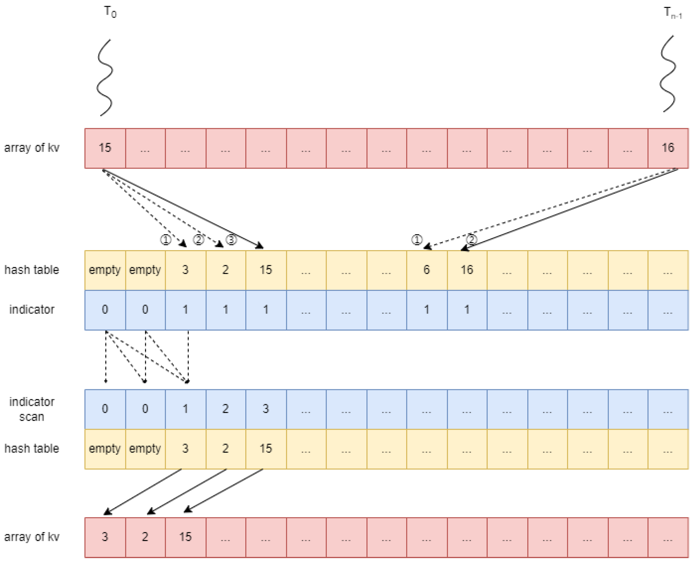
4.1.1. Phase 1: No Probe Hash into Partial Hash Table

First, we clarify the roles of the three arrays in this stage. The red array is utilized to store the key-value pairs, while the blue array serves as an indicator of whether the key-value pairs in the red array have been inserted into the hash table. If a key-value pair located at index i in the red array has been inserted into the hash table, then the i-th item in the blue array is set to 0; otherwise, it is set to 1. The yellow array is divided into three parts: the first part functions as the hash table during this stage, the second part acts as the hash table indicator (where the i-th item in the hash table indicator is set to 1 if the corresponding slot in the hash table is not empty), and the third part remains unused in this stage.

Next, we describe the process of this stage. Each thread is responsible for a key-value pair and calculates the hash value of the key. Let us denote the hash value of the key as $hv$. Each thread $T_i$ computes the insertion position via $hvmodL$ and attempts insertion. There are three possible scenarios:

• The insertion location is not within the first part of the yellow array.
• The insertion location is within the first part of the yellow array, but a key is already present at that location.
• The insertion location is within the first part of the yellow array, and no key is present at that location.

In scenarios (1) and (2), the key is not inserted into the hash table, and the indicator is set to 1. In scenario (3), the key is inserted into the hash table, and the indicator is set to 0.

4.1.2. Phase 2: Collect Key/Value in Hash Table

In this stage, only the yellow array is utilized. The first two parts of the yellow array function similarly to the previous stage, while the third part is designated for collecting key-value pairs from the hash table. To determine where each key-value pair should be collected, we first perform an in-place scan of the hash table indicator. Subsequently, we utilize $L/3$ threads to collect key-value pairs from the hash table, with each thread responsible for one item in the hash table. For thread $T_i$, it first checks whether the key is empty; if it is empty, the thread returns immediately. If it is not empty, the thread reads the i-th item in the hash table indicator, which indicates the collection location of the key-value pair, and collects the key-value pair into the collection array.

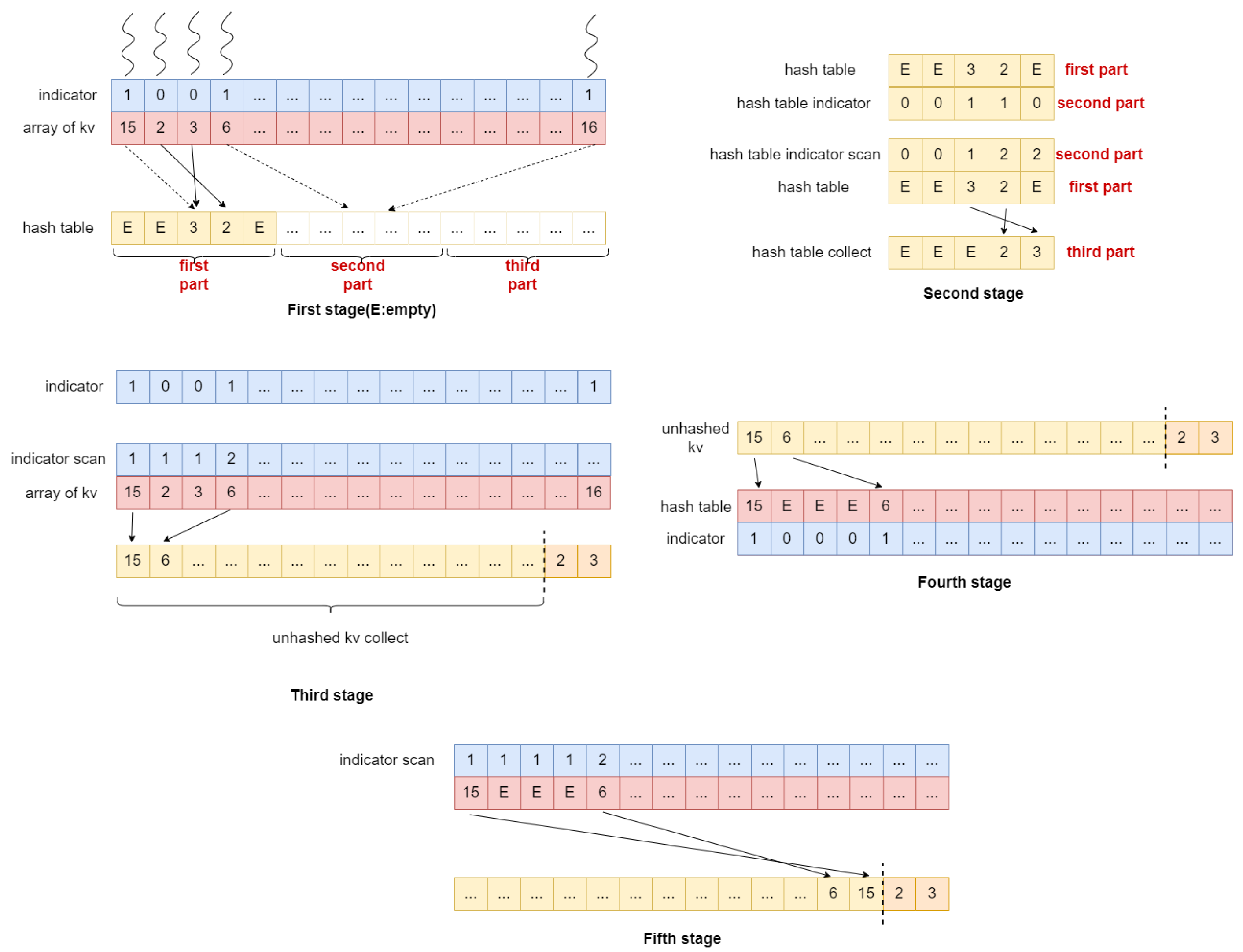
4.1.3. Phase 3: Collect Unhashed Key/Value Pairs

In this stage, the blue and red arrays function similarly to the first stage. The right part of the yellow array is used to collect key-value pairs from the last stage, while the remaining part is used to collect key-value pairs that were unhashed in the first stage. The process is analogous to that of the second stage. We first perform an in-place scan of the key-value indicator array. Each thread is responsible for one key-value pair in the key-value array. For thread $T_i$, it first checks if the key-value pair is unhashed by evaluating the result of $\mathrm{indicator}\left[i\right]-\mathrm{indicator}[i-1]$. If the result equals 1, then this key-value pair is considered unhashed. If the key-value pair is unhashed, it is collected into the collection array based on the i-th item of the indicator scan result; otherwise, $T_i$ returns immediately.

4.1.4. Phase 4: Hash Aggregate Remaining Key/Value Pairs Using Linear Probe

In this stage, the unhashed key-value pairs have been collected into the left part of the yellow array. This stage aims to hash aggregate these key-value pairs. The red array serves as the hash table, while the blue array functions as the hash table indicator. Each thread is responsible for one key-value pair in the key-value array. For thread $T_i$, it first calculates the hash value of the key. Let us denote the hash value as $hv$. The thread $T_i$ then calculates the insertion location in the hash table using $hvmodL$ and attempts to insert the key-value pair at this location. There are three possible scenarios:

• The key at the insertion location is empty.
• The key at the insertion location is the same as the key that $T_i$ is responsible for.
• The key at the insertion location is different from the key that $T_i$ is responsible for.

In scenario (1), $T_i$ inserts the key-value pair into the hash table and sets the indicator to 1. In scenario (2), $T_i$ aggregates the value with the value in the hash table. In scenario (3), $T_i$ linearly probes the hash table to find an empty position, which leads it back to scenario (1).

4.1.5. Phase 5: Collect Key/Value Pairs in Hash Table and Combine with Previous Results

This stage is similar to the second stage. We first perform an in-place scan of the hash table indicator (blue array). Then, we collect the key-value pairs from the hash table (red array) based on the scan results and place them into positions that are close to the corresponding positions in the collection array (yellow array) from the second stage.

4.1.6. Summary

In stages one to two, SP-EGA does not perform linear probing but instead ignores the key-value pairs that require probing. This has two benefits: first, for a significant portion of key-value pairs, we do not perform linear probing; second, in the remaining stages, we have already generated some GA results (in stage one to two), which we can temporarily store and then clear the hash table. This way, when we perform GA on the remaining key-value pairs (stages three to five), since the hash table size is sufficiently large relative to the remaining key-value pairs, even if we use linear probing at this point, it will not result in excessively long probing distances. Longer probing distances mean more atomic operations, which are very costly for GPUs and can even be considered the primary overhead in the GPU GA. Through the algorithm design of SP-EGA, we significantly reduce the average probing distance for all key-value pairs. Although we need to incur some additional data movement to combine the GA results from the two stages, it is worthwhile.

4.2. MP-EGA

Consider a scenario where the volume of data exceeds the storage capacity of the GPU. In such cases, SP-EGA is no longer applicable. A viable solution is to segment the data into multiple partitions, ensuring that each partition fits within the GPU’s memory constraints. In this scenario, we designed the MP-EGA algorithm. Below, we first discuss the key design points of MP-EGA and then present the algorithm flow of MP-EGA.

Determining the optimal number of partitions is crucial. If the number of partitions is too small, some partitions may not fit into the GPU memory, leading to inefficiencies. Conversely, if the number of partitions is excessively large, we may not fully utilize the GPU’s computational capabilities. Therefore, we need a partitioning strategy that achieves balance between memory constraints and computational efficiency. Even if we choose the right number of partitions, there may still be some partitions that are too large or too small (depending on the key/val pairs distribution). We need strategies to handle these partitions that are too large or too small. Since MP-EGA is a heterogeneous algorithm, it needs to copy data back and forth between the CPU and the GPU. Thus, we need a way to reduce copying overhead.

4.2.1. Using Balls into Bins Model to Determine Number of Partitions

We can partition the data into P partitions, ensuring that each partition fits within the GPU memory, which reduces the problem to that discussed in the previous section. However, determining the optimal number of partitions is critical. Too many partitions result in smaller partition sizes, leading to insufficient GPU utilization. Additionally, an excessive number of partitions increases the number of GPU kernel invocations, which raises the fixed costs associated with these invocations. Conversely, too few partitions lead to larger partition sizes, potentially exceeding the GPU memory limits.

Although we cannot guarantee that each partition will fit within GPU memory, it is acceptable for only a very small portion of partitions to exceed this limit. Intuitively, increasing the number of partitions reduces the probability of any single partition exceeding GPU memory. We can analyze this problem using the “balls into bins” model, where we consider the group of key-value pairs as balls and the partitions as bins. Given the limited GPU memory, the number of groups in each partition is also constrained.

Let k represent the maximum number of groups allowed in each partition. Our goal is to ensure that the number of balls (key-value pairs) in each bin (partition) remains below k. While we cannot guarantee that the number of balls in some bins will not exceed k, we aim to keep the probability of this occurrence very low. Intuitively, as we increase the number of bins, the probability of any single bin exceeding k diminishes.

The question then arises: how many bins are sufficient? We have established the following theorem to address this question.

Theorem 1.

Consider n balls randomly distributed across m bins. k is a positive integer greater than 1. p is a real number greater than 0 and less than 1. Let $m_0=e^{{\displaystyle \frac{kln\frac{ne}{k}-lnp}{k-1}}}$. If $m\ge \lceil m_0\rceil$, then we have

$$Pr\left[allbinshaveatmostk-1balls\right]\ge 1-p.$$

Proof. 

First, let us define some events as follows: $A_i$: “bin i has at least k balls”, $B_{ij}$: “the $j^{th}$ subset whose size is k of n balls falls into the $ith$ bin”, C: “at least one bin has at least k balls”, D: “all bins have at most $k-1$ balls”.

Suppose n balls have s subsets whose size are k; it is obvious that $s=\left({\displaystyle \genfrac{}{}{0pt}{}{n}{k}}\right)$. We can conclude that $A_i\subset {\bigcup }_{j\in \{1,2,\dots ,\left({\displaystyle \genfrac{}{}{0pt}{}{n}{k}}\right)\}}{B}_{ij}$, so we have $Pr\left[A_i\right]\le {\sum }_{j=1}^{\left({\displaystyle \genfrac{}{}{0pt}{}{n}{k}}\right)}Pr\left[B_{ij}\right]={\displaystyle \frac{\left(\genfrac{}{}{0pt}{}{n}{k}\right)}{m^k}}$.

Since $C\subset {\bigcup }_{i=1}^m{A}_i$, we have

$$Pr\left[C\right]\le Pr\left[{\bigcup }_{i=1}^m{A}_i\right]\le {\sum }_{i=1}^{m}Pr\left[A_i\right]=m{\displaystyle \frac{\left(\genfrac{}{}{0pt}{}{n}{k}\right)}{m^k}}$$

(1)

Since we desire that $Pr\left[D\right]\ge 1-p$ and we have $Pr\left[D\right]=1-Pr\left[C\right]$, it is equivalent to prove

$$Pr\left[C\right]\le p$$

(2)

From (1) and (2), we know that if we can prove that

$$m{\displaystyle \frac{\left(\genfrac{}{}{0pt}{}{n}{k}\right)}{m^k}}\le p$$

(3)

then we could prove (2).

From Stirling’s approximation, we have

$$k!\ge {\left({\displaystyle \frac{k}{e}}\right)}^k$$

(4)

Then we have

$$\left({\displaystyle \genfrac{}{}{0pt}{}{n}{k}}\right)={\displaystyle \frac{n(n-1)\dots (n-k+1)}{k!}}\le {\displaystyle \frac{n^k}{k!}}\le {\left({\displaystyle \frac{ne}{k}}\right)}^k$$

(5)

From (3) and (5), we know that we should prove

$${\left({\displaystyle \frac{ne}{k}}\right)}^k\le p{m}^{k-1}$$

(6)

Taking the logarithm of both sides of inequality (6), we obtain

$$kln{\displaystyle \frac{en}{k}}\le lnp+(k-1)lnm$$

(7)

Suppose $f\left(m\right)=(k-1)lnm+lnp-kln{\displaystyle \frac{en}{k}}$, then inequality (6) is equivalent to $f\left(m\right)\ge 0$. Since the function f is monotonically increasing (for $k>1$), and we have ${lim}_{m\to 0}f\left(m\right)=-\infty$ and ${lim}_{m\to +\infty }f\left(m\right)=+\infty$, there must exist $m_1$ such that

$$f\left(m_1\right)=0$$

(8)

We can verify that $m_1=m_0$. Thus, we conclude that if $m\ge \lceil m_0\rceil$, then $Pr\left[\mathrm{all}\mathrm{bins}\mathrm{have}\mathrm{at}\mathrm{most}k-1\mathrm{balls}\right]\ge 1-p$.    □

Using this theorem, we can determine the sufficient number of partitions. Assuming our hash function distributes the data randomly across partitions, we can set p to a very small value and choose the partition number as $\lceil m_0\rceil$. This approach ensures that the probability of any partition exceeding GPU memory remains very low.

4.2.2. Using Feedback Load to Handle Large Partitions

Assuming we partition the data based on the hash values of the keys, the unknown distribution of the data may result in some partitions being too large for GPU memory. In this case, we must consider how to process large partitions efficiently. One approach is to handle such partitions on the CPU; however, even if the partition is too large for the CPU memory, the GA results might still fit within GPU memory; thus, this method might miss the opportunity to leverage GPU processing, which could lead to performance degradation. Alternatively, processing the partition on the GPU may be viable, but if the GA results exceed GPU memory, we would need to reprocess the partition, incurring additional performance costs.

First, we must recognize that even if the partition size exceeds GPU memory, the GA results may still fit within the available GPU memory. Therefore, we need a method to determine whether the GA results within a partition exceed the GPU global memory limit. A natural approach is to load key-value pairs into GPU memory that correspond to the available free space in the hash table and then calculate the GA result. This process is repeated until either all key-value pairs fit in GPU memory or the hash table is full, leaving some key-value pairs unprocessed.

However, a limitation of this method is that, in later rounds, the free space in the hash table may become very small, which means fewer and fewer key-value pairs are transferred between the CPU and GPU, resulting in inefficient use of PCIe bandwidth and GPU computational resources.

Our solution introduces a dynamic memory reservation strategy that strategically allocates overflow buffers through a feedback-driven control mechanism. This approach achieves high device utilization with relatively low space overhead. We define two threshold values for the hash table: $L{F}_{\min }$ and $L{F}_{\max }$. Here, $L{F}_{\min }$ represents the minimum acceptable load factor, while $L{F}_{\max }$ denotes the maximum load factor.

In each iteration, we first calculate how many additional key/value pairs can be loaded into the hash table based on $L{F}_{\max }$ and the number of key/value pairs already present in the hash table. We then compute the GA results for the newly loaded key/value pairs. If the number of results exceeds the $L{F}_{\min }$ threshold, we consider the hash table to be “full”, then we process the remaining key/value pairs on the CPU. Conversely, if the result count is below the $L{F}_{\min }$ threshold, we conclude that the hash table is not full and can continue loading key/value pairs based on the $L{F}_{\max }$ threshold and the current result count.

This process is repeated until all key/value pairs fit in GPU memory or the hash table is full, leaving some key/value pairs that are processed in a CPU. In each round, we ensure that the minimum data transfer volume between the CPU and GPU is no less than $(L{F}_{\max }-L{F}_{\min })\times \mathrm{HASH}\_\mathrm{TABLE}\_\mathrm{SIZE}$. By avoiding excessively small data transfer volumes between the GPU and CPU, we can more fully utilize the PCIe bandwidth.

4.2.3. Using Greedy Merge to Handle Small Partitions

When many partitions are generated, some may be very small, which is inefficient for GPU processing. Thus, it is necessary to merge small partitions into larger ones. We formalize the partition merging problem through the following mathematical framework: Let all partitions form a set, with the assumption that no partition’s size exceeds k (due to the limitations imposed by GPU global memory capacity). We can merge two partitions if the sum of their sizes is less than k. The challenge lies in merging partitions such that the total number of merged partitions is minimized. A naive approach that traverses all merging possibilities would result in unacceptable time complexity, necessitating the development of a more efficient solution.

Our core idea is to merge the two smallest partitions. The algorithm terminates when the merge size of these two partitions exceeds k. The detailed algorithm is as follows: we first construct a min-heap based on partition sizes. If the heap size is equal to 1 or the merge size of the two smallest partitions exceeds k, we terminate the algorithm. Otherwise, we pop the two smallest partitions, merge them into a new partition, and continue merging the current smallest partition until the next merge would exceed k. This process is repeated until the algorithm terminates. The pseudocode for our algorithm can be found in Algorithm 1.

Next, we will demonstrate the efficiency of the algorithm through the following theorem.

Theorem 2.

Suppose $A=\{a_1,a_2,\dots ,a_n\}$, $1\le a_i\le K$, $a_i\in {\mathbb{N}}^{+}$, $1\le i\le n$. Now, divide A into x disjoint subsets $B_1,B_2,\dots ,B_x$ such that $\forall j\in \{1,2,\dots ,x\},{\sum }_{b\in B_j}b\le K$. We call this process a cut, and we define the degree of the cut as x. A cut is optimal if its degree is the smallest among all cuts. Suppose that the optimal cut is $\mathbb{B}$; then, we can find a cut $\mathbb{C}$ whose degree is y and $y<2x$ in $O(nlogn)$ time complexity.

Proof. 

Since the total number of partitions is limited, we know that the optimal cut must exist. Suppose that the optimal cut is $\mathbb{B}:B_1,B_2,\dots ,B_x$. In the initial situation, we can assume that set A is divided into n parts: $C_1,C_2,\dots ,C_n$, where $C_i=\left\{a_i\right\}$, $1\le i\le n$. So the initial cut is ${\mathbb{C}}_0:C_{0,1},C_{0,2},\dots ,C_{0,n_0}$. Suppose $C_{i,1},C_{i,2},\dots ,C_{i,n_i}$ are sorted by $\mathrm{Sum}\left(C_{i,j}\right)$ in ascending order. Let ${\sum }_{k=1}^j\mathrm{Sum}\left(C_{i,k}\right)\le K$ and ${\sum }_{k=1}^{j+1}\mathrm{Sum}\left(C_{i,k}\right)>K$. Then, we merge $C_{i,1},\dots ,C_{i,j}$ into one set and obtain the new cut ${\mathbb{C}}_{i+1}$.

Suppose that after t such iterations, we obtain the cut ${\mathbb{C}}_t$, which satisfies $\mathrm{Sum}\left(C_{t,0}\right)+\mathrm{Sum}\left(C_{t,1}\right)>K$. The degree of cut ${\mathbb{C}}_t$ is y. Let $S={\sum }_{k=1}^y\mathrm{Sum}\left(C_{t,k}\right)$. Then,

$$2S=\sum _{k=1}^y\left(\mathrm{Sum}\left(C_{t,k}\right)+\mathrm{Sum}\left(C_{t,y+1-k}\right)\right).$$

Since $\mathrm{Sum}\left(C_{t,k}\right)+\mathrm{Sum}\left(C_{t,y+1-k}\right)\ge \mathrm{Sum}\left(C_{t,0}\right)+\mathrm{Sum}\left(C_{t,1}\right)>K$, we have $2S>yK$.

Since $S={\sum }_{k=1}^x\mathrm{Sum}\left(B_k\right)$ and $\mathrm{Sum}\left(B_k\right)\le K$, we have $2S\le 2Kx$. Combining $2S>yK$ and $2S\le 2Kx$, we obtain $yK<2Kx$, which implies $y<2x$. So ${\mathbb{C}}_t$ is the cut we found.

Now, let us analyze the time complexity. In every iteration, we merge at least two sets, so the degree of the new cut decreases by at least 1. The initial degree is n, so the number of iterations is $O\left(n\right)$. In each iteration, we insert the merged set into an ordered set list, and the time complexity of this operation is $O(logn)$. Initially, we sort the initial cut, which has a time complexity of $O(nlogn)$. Therefore, the overall time complexity is $O(nlogn)$.    □

Algorithm 1: Partition Merge Algorithm

4.2.4. Using Multi-Stream to Hide Copy Latency

In this scenario, where the volume of data exceeds the storage capacity of the GPU, data must be copied from the CPU to the GPU and vice versa. If data copying and processing occur sequentially, copy latency may become a bottleneck in the overall process. To mitigate this, we need to explore strategies that allow for overlapping data transfer and computation, thereby hiding copy latency and improving overall performance.

In CUDA, a stream is defined as a sequence of commands that are executed in order. Commands within different streams can be executed concurrently, enabling efficient utilization of GPU resources.

To mitigate copy latency, we can leverage multiple streams. Since the key/value pairs in different partitions are independent, we can allocate one stream to process one partition. Each stream is managed by a dedicated CPU thread. The CPU thread first copies data from the CPU to the GPU, then the GPU processes the data and subsequently transfers the results back to the CPU.

This approach allows for overlapping data transfer and computation: while one stream is engaged in copying data between the CPU and GPU, another stream can simultaneously process data on the GPU. Consequently, this strategy effectively hides copy latency, enhancing overall performance and throughput.

4.2.5. MP-EGA Algorithm Flow

Based on the above discussions, we can comprehensively describe the algorithm flow of MP-EGA. The algorithm is divided into two phases: the partition-generating phase and the partition-processing phase.

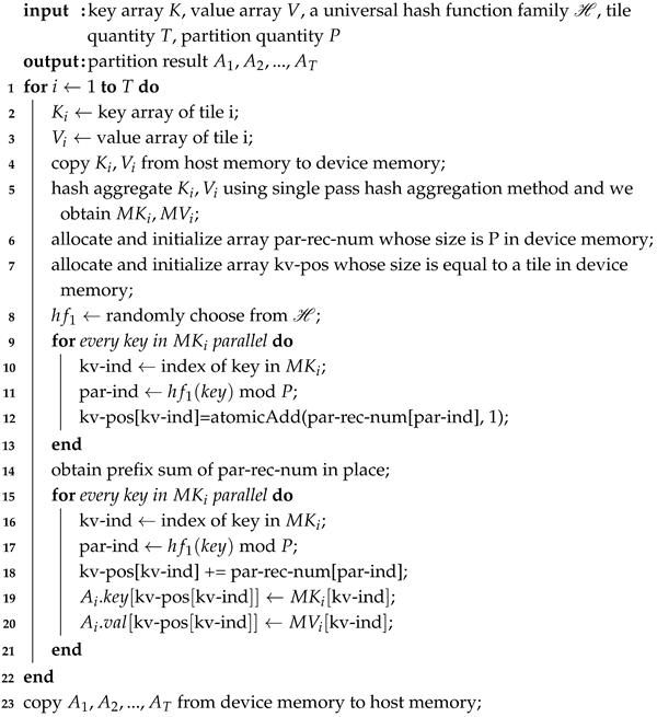
The partition-generating phase is shown in Figure 3. The pseudo code of this phase can be referred to in Algorithm 2. Suppose the key/val array is stored in the CPU memory, we divided the key/val array into T tiles such that each tile could be processed in GPU memory. Each tile is either processed by a GPU or CPU. In a CPU, each tile is processed by t threads. In a GPU, each tile is processed by a CUDA stream and we have s CUDA streams in order to hide copy latency. Next, we will clarify how a CPU and GPU will process the tile.

In the GPU, we could focus on one stream since each stream does the same thing. In each stream, we first copy the key/val array from a CPU to GPU, and then we process the key/val tile using the SP-EGA. After we obtain the GA results, we could compute the partition results. Three CUDA kernels are used to compute the partition result.

The first kernel computes the index within the partition for each key/value pair. Each thread block is responsible for a subset of key/value pairs in the tile. Given P partitions, each GPU thread atomically increments the counter of the partition to which the key/value pair belongs, yielding the index of each key/value pair within the thread block. We then atomically increment the global counter of the partitions to obtain the index of each key/value pair within the partition. The second kernel computes the prefix sum of the global counters of the partitions. The third kernel calculates the final index of each key/value pair within the tile by adding the index within the partition (computed by the first kernel) to the global position of the partition (computed by the second kernel).

Algorithm 2: MP-EGA partition algorithm

In the CPU, we can focus on a single thread since each thread performs the same operations. Each thread is responsible for a subset of key/value pairs in a tile and maintains a local partition counter array. For each key/value pair, we first determine the partition it belongs to, increment the local partition counter, and obtain the local index within the partition. Each thread is responsible for specific partitions and can add its local partition counter to the global partition counter, yielding the position of the local partition in the global context. We then compute the global index of each key/value pair within the partition by adding the local index within the partition to the global position of the partition. Finally, we scan the global partition counter to determine the position of each partition in the final result, allowing us to compute the final index of each key/value pair by adding the global index within the partition to the position of the partition.

After processing all tiles, each tile produces its own partition result. However, some partition results may be too small. To address this, we can merge the results of smaller partitions into larger ones. The partition merge algorithm is outlined in the accompanying algorithm.

Each partition result is distributed across the partition results of each tile. Consequently, copying a single partition to the GPU may require multiple transfers, specifically T copies, which can hinder the efficient utilization of PCIe bandwidth. Therefore, we first merge the partition results on the CPU before proceeding to the next phase.

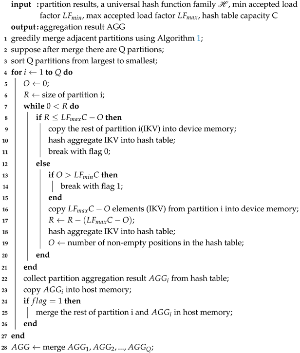
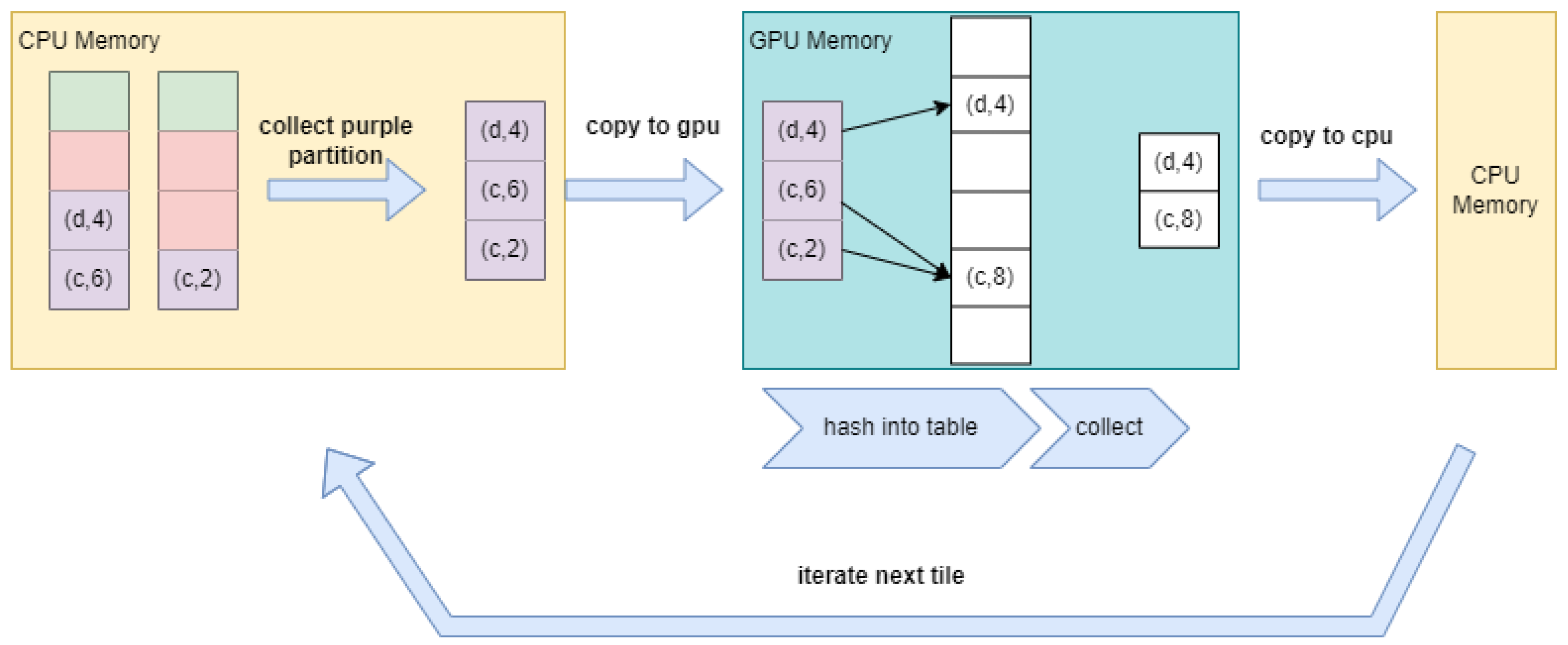
Next, we introduce the partition-processing phase, as illustrated in Figure 4. The pseudo code for this phase can be referred to in Algorithm 3. In this phase, each partition is processed using a CUDA stream. For simplicity, we will focus on the operations occurring within a single stream. Initially, we copy the partition result from the CPU to the GPU. It is important to note that the size of the partition result is not fixed, unlike the size of the key/value tiles in the partition-generating phase.

Algorithm 3: MP-EGA partition process algorithm

    We must consider two scenarios: when the size of the partition result fits within GPU memory and when it exceeds GPU memory. If the partition result fits in GPU memory, we can directly process it on the GPU. Conversely, if the partition result exceeds GPU memory, we will employ the method described in the section titled “Using Feedback Load to Handle Large Partitions”. In cases where the partition is too large for the GPU, we will process the remaining key/value pairs on the CPU and combine these results with those computed on the GPU. After processing all partitions, we will obtain the final results.

5. Results

We conducted experiments under two scenarios: (1) data fitting within GPU memory for single-pass processing, and (2) data exceeding GPU memory capacity.

5.1. Setup

We conducted our experiments on an Ubuntu server equipped with an Intel(R) Xeon(R) Gold 6230R CPU (Intel Corporation, Santa Clara, CA, USA), an A100 PCIe 40 GB GPU, and 192 GB of memory. All code was compiled using CUDA 12.3 and GCC 11.4.0. To evaluate performance, we used the following GA query:

SELECT K, AGG(V)

FROM (K, V)

GROUP BY K

5.1.1. Workload Description

In scenarios where the data volume can fully fit into the GPU, we evaluate the performance of each algorithm on the relation $R(k,v)$, where k is the key for grouping and v represents the value used for aggregation. The number of records in relation R is 100 million, and the data types for k and v are UINT32. For the groupby aggregation operator, the number of data groups is a critical factor affecting performance. By adjusting the number of unique groups (1–100% of total entries), we systematically tested hash-table load factors from 0.01 to 1.0. To compare the impact of the number of data groups on algorithm performance, we need to control the data distribution. Referring to previous work, the elements in relation R are drawn from a uniform distribution [12]. This isolates algorithmic performance from data-specific optimizations. Extreme skews (e.g., Zipfian distributions) or sparse keys may affect the performance of the algorithm. Therefore, to test the impact of data distribution on algorithm performance, we also generated a workload that keeps the number of control data groups unchanged but alters the data distribution. We chose the Zipfian distribution, where the skew factor parameter can be adjusted to control the degree of data distribution imbalance. Our skew factor can take values of 0.2, 0.4, 0.6, and 0.8.

In scenarios where the data volume exceeds the GPU memory capacity, we selected datasets with 1 billion and 2 billion data points to reflect real-world “big data” scenarios, aligning with our focus on GPU memory constraints and large-scale processing. In this scenario, the number of data groups also affects algorithm performance, so our dataset is configured with 10 million, 100 million, and 1 billion groups to test the algorithm’s performance under different group counts.

5.1.2. Baselines

In scenarios where the data volume can fully fit into the GPU, the SOTA algorithm for hash-based array grouping and aggregation acceleration is LPHGA [12]. For sortingbased SOTA algorithms, we chose to compare with cuDF (v25.04.00), a GPU-accelerated library for data analysis developed by NVIDIA, which integrates SOTA implementations of sorting-based group aggregation [29].

In scenarios where the data volume exceeds the GPU memory capacity, since we have not found a GPU DBMS that supports GA of data larger than the GPU memory, we compare our method MP-EGA with high-performance CPU DBMS DDB(DuckDB), which supports the SOTA implementation of the CPU GA algorithm.

5.2. SP-EGA VS LPHGA VS cuDF

The results are illustrated in the Figure 5.

We can observe that SP-EGA and cuDF maintain relatively stable performance under different load factors, while the performance of LPHGA drops sharply when the load factor exceeds 0.9. When the load factor is less than 0.90, the performance of LPHGA and SP-EGA is similar. However, when the load factor exceeds 0.90, SP-EGA achieves a speedup ratio of 1.16× to 5.39× compared to LPHGA, with higher load factor yielding greater speedup ratio. And when the load factor changes from 0.01 to 0.99, SP-EGA can achieve a speedup ratio of 1.30× to 2.48× compared to cuDF.

To test the impact of data distribution on the performance of the three algorithms, we fixed the load factor at 0.95 and evaluated the performance of the three methods under uniform distribution and Zipfian distributions with skew factors of 0.2, 0.4, 0.6, and 0.8, as shown in the Figure 6. We can see that the performance of SP-EGA and cuDF remains relatively stable under different data distributions, while the performance of LPHGA fluctuates significantly.

5.3. Probe Number of SP-EGA and LPHGA

To further verify that SP-EGA indeed reduces the number of linear probes compared to LPHGA, we record the average probe number of two algorithms under different load factors in

Table 1. Average probe number of SP-EGA and LPHGA under different load factor.

Load Factor	SP-EGA	LPHGA
0.91	1.66	5.64
0.92	1.71	6.32
0.93	1.76	7.18
0.94	1.81	8.36
0.95	1.86	9.97
0.96	1.92	12.52
0.97	1.99	16.69
0.98	2.06	25.30
0.99	2.13	53.56

. When the load factor changes from 0.91 to 0.99, the probe number of SP-EGA changes from 1.66 to 2.13. It can be seen that the probe number of SP-EGA is relatively stable. However, the probe number of LPHGA changes from 5.64 to 53.56. It can be seen that the probe number of LPHGA increases rapidly. Excessive numbers of probes lead to poor performance of LPHGA under high load factors.

5.4. MP-EGA VS DDB

In this experiment, we compared the performance of MP-EGA with DDB under different data volume and different group number. The result is shown in Figure 7. We could see that MP-EGA outperforms DDB in all cases. The speedup ratio of MP-EGA compared to DDB ranges from 6.45× to 29.12×. When we fix the dataset size (e.g., only looking at the dataset of size 1 billion), we can observe that as the number of data groups (cardinality) decreases from 1 billion to 10 million, the GA time of MP-EGA reduces from 5.64 s to 1.61 s, resulting in a performance improvement of 3.5 times. This shows that MP-EGA’s performance significantly improves as the number of data groups decreases. But for DDB, the performance remains basically unchanged. This is because the performance bottleneck of MP-EGA is the PCIE bandwidth. When the number of data groups is reduced, the partition results will also be reduced, which means that the amount of data that needs to be copied between the CPU and the GPU will also be reduced, so the performance of MP-EGA is significantly improved. We will analyze the performance bottleneck of MP-EGA in detail in the next section. On the other hand, when we fix the number of data groups and increase the size of the dataset from 1 billion to 2 billion, the time consumed by MP-EGA becomes about 2 times, while the time consumed by DDB becomes about 3 times, which also shows that the scalability of MP-EGA is better than that of DDB.

5.5. Time Breakdown of MP-EGA

We divided the time consumed by MP-EGA into six parts: copy in and out (partitiongenerating phase), SP-EGA (partitiongenerating phase), calculate partition result (partition-generating phase), collect partition result (partition-processing phase), copy in and out (partition-processing phase), and calculate final result (partition-processing phase). In order to calculate the time proportion of each part, there is only one CUDA stream used in this experiment (to prevent the overlapping of time segments in multi-stream scenarios). We randomly generated 10 billion key/val pairs, and the time proportion of each part was tested with the number of data groups set to 1 billion, 5 billion, and 10 billion. The result is shown in Figure 8. It can be seen that the time proportion of each part is basically the same under different data groups. The parts related to data copy between the CPU and the GPU are: copy in and out (partition-generating phase), copy in and out (partitionprocessing phase), and collect partition result (partition-processing phase). These parts account for about 68.2% of the total time. This shows that the bottleneck of MP-EGA lies in PCIE bandwidth. In a multi-stream scenario, SP-EGA (partition-generating phase) and calculate partition result (partition-generating phase) basically overlap with the copy in and out (phase 1). The time breakdown result explains why we need to perform SP-EGA in the first stage instead of just calculating the partition results. Because even if there is no SP-EGA in the partition-generating phase, the time consumed by the copy in and out (partition-generating phase) will not be reduced, thus the overall time of partitiongenerating phase will not be reduced. But if there is SP-EGA in the partition-generating phase, the time consumed by the copy in and out (partition-generating phase), collect partition result (partition-processing phase), and copy in and out (partition-processing phase) may be reduced since partition results may contain fewer key/val pairs. This is why the performance of MP-EGA is significantly improved when the number of data groups is reduced.

6. Discussion

6.1. Contextualizing Performance Improvements

Our experimental findings reveal two key advancements in GPU-accelerated groupby aggregation (GA). First, SP-EGA’s ability to maintain 1.16–5.39× speedup over LPHGA under high load factors (0.9–1.0) addresses a critical limitation in hash-based GPU algorithms identified by Karnagel et al. [1]. While prior work [12] emphasized load factor constraints through linear probing optimization, our two-phase aggregation strategy fundamentally reconfigures collision resolution mechanics. This aligns with Tome et al.’s vision of adaptive GPU operators [20], but extends it through algorithmic rather than configuration-space optimization.

Second, MP-EGA’s 6.45–29.12× acceleration over CPU-based DuckDB demonstrates the viability of out-of-core GPU processing—a capability absent in existing GPU DBMS implementations like HeavyDB [26] and BlazingSQL [27]. This breakthrough responds directly to Rosenfeld et al.’s [11] call for scalable GPU query operators in big data contexts.

6.2. Mechanistic Insights from Probe Analysis

The probe count data (Table 1) provides mechanistic validation of SP-EGA’s design rationale. At a load factor of 0.99, SP-EGA reduces the average probes by 96% compared to LPHGA (2.13 vs. 53.56). This supports our hypothesis that partial aggregation stages mitigate linear probing’s degenerative behavior. The results empirically confirm Amenta et al.’s [19] theoretical analysis of hash table performance degradation patterns.

6.3. Architectural Implications

Our multi-stream pipeline design (Figure 4) overcomes PCIe bandwidth limitations through three innovations: (1) overlapping computation with data transfer, (2) dynamic partition merging via Algorithm 1, and (3) feedback-driven load balancing. This advances Kaldewey et al.’s [22] foundational work on CPU–GPU coprocessing by introducing data volume awareness into scheduling decisions.

6.4. Theoretical Contributions

Our work makes three layered contributions:

• Algorithmic Innovation: Demonstrated that multi-stage partial aggregation enables full-load-factor hash tables (SP-EGA), challenging the 0.5 load factor paradigm [1].
• System Design: Established a balls-into-bins probabilistic model (Section 4.2.1) for GPU memory-aware partitioning.
• Architectural Principle: Showed that feedback-controlled data staging (Section 4.2.2) can mitigate PCIe bottlenecks in heterogeneous systems.

These advancements collectively address He et al.’s [2] identified gap in real-time GPU analytics capabilities while providing a template for adapting other memory-intensive operators to out-of-core GPU environments.

7. Conclusions

This study addresses two critical challenges in GPU-accelerated GA: performance degradation under high hash table load factors (LF > 0.9) and the inability to process datasets exceeding GPU memory capacity. Through algorithmic innovation, we propose EGA—a dual-mode framework consisting of Single-Pass EGA (SP-EGA) for in-memory scenarios and Multi-Pass EGA (MP-EGA) for out-of-core computations.

Three key advancements emerge:

• Mechanism Design: SP-EGA reduces average probe distance by 60–95% compared to LPHGA through a two-phase hashing strategy (no-probe insertion followed by linear probing), achieving stable performance even at LF = 1.0.
• Scalability Innovation: MP-EGA introduces a probabilistically guaranteed partitioning model based on “balls-into-bins” theory, combined with greedy merging and multi-stream pipelining, enabling efficient GA on datasets 50× larger than GPU memory.
• Performance Leap: Experimental validation demonstrates SP-EGA achieves 1.16–5.39× speedup over SOTA hash-based GPU method LPHGA under high-LF scenarios and achieves 1.30–2.48× speedup over SOTA sort-based GPU method cuDF, while MP-EGA outperforms CPU-based DuckDB by 6.45–29.12× on billion-scale datasets.

Our work redefines three paradigms in GPU–GA research: 1. Load Factor Tolerance: Challenges the long-standing “LF ≤ 0.5” design rule, proving that high-density hash tables can maintain efficiency through probe optimization; 2. Heterogeneous Workflow: Establishes a CPU–GPU co-processing template using feedback-driven load balancing ($L{F}_{min}/L{F}_{max}$ thresholds), reducing PCIe transfer overhead by 42% compared to static partitioning; 3. Algorithmic Generality: The probabilistic partition sizing model (Theorem 1) provides a mathematical foundation for out-of-core GPU algorithms beyond GA.

Practically, EGA’s latency reduction in billion-row aggregation (Figure 7) directly enables real-time analytics in the following: financial fraud detection systems requiring sub-second response on TB-scale transaction logs; IoT platforms processing high-velocity sensor data with strict SLAs; edge computing deployments where GPU resources are memory-constrained.

While EGA significantly advances GPU–GA, two limitations open new research avenues:

• Atomic Operation Dependency: The remaining 31.8% of non-overlapped computation time (Figure 8) stems from atomic synchronization. Future work will explore lock-free hashing using NVIDIA Hopper’s thread block clusters.
• Operator Extensibility: Although optimized for groupby aggregation, extending EGA’s paradigm to JOIN and WINDOW functions could revolutionize GPU-based SQL engines—a direction we are actively pursuing.

These advancements provide a robust solution for large-scale data analysis tasks, enabling real-time processing capabilities that are critical in domains such as finance, healthcare, and social media analytics. Looking ahead, future work will explore synchronization mechanisms beyond atomic instructions to further enhance performance, as well as extend our acceleration techniques to other big data operations, such as join operations, to broaden the applicability of GPU acceleration in data analysis.

We provide our source code at https://github.com/PneNPproof/cpu_gpu_coprocess_groupby_agg (accessed on 1 February 2025).