
A Two-Step Algorithm for Handling Block-Wise Missing Data in Multi-Omics


Abstract
1. Introduction
2. Methods
2.1. Block-Wise Missingness and Profiles
2.2. Two-Step Optimization Procedure
2.2.1. Computing When Is Fixed
2.2.2. Computing When Is Fixed
2.2.3. Two-Stage Algorithm
| Algorithm 1 Two-stage iterative solution for and . |
Input: , , , ⟶ Output: Solutions and to (4)
|
3. Multi-Class Classification
3.1. Computing When Is Fixed
3.2. Computing When Is Fixed
4. Results
4.1. Breast Cancer Data
4.2. Exposome Data
5. Discussion
6. Conclusions
Author Contributions
Funding
Data Availability Statement
Acknowledgments
Conflicts of Interest
References
- The Cancer Genome Atlas Research Network; Weinstein, J.N.; Collisson, E.A.; Mills, G.B.; Shaw, K.R.; Ozenberger, B.A.; Ellrott, K.; Shmulevich, I.; Sander, C.; Stuart, J.M. The cancer genome atlas pan-cancer analysis project. Nat. Genet. 2013, 10, 1113–1120. [Google Scholar]
- Chierici, M.; Bussola, N.; Marcolini, A.; Francescatto, M.; Zandonà, A.; Trastulla, L.; Agostinelli, C.; Jurman, G.; Furlanello, C. Integrative network fusion: A multi-omics approach in molecular profiling. Front. Oncol. 2020, 10, 1065. [Google Scholar] [CrossRef]
- Picard, M.; Scott-Boyer, M.P.; Bodein, A.; Périn, O.; Droit, A. Integration strategies of multi-omics data for machine learning analysis. Comput. Struct. Biotechnol. J. 2021, 19, 3735–3746. [Google Scholar] [CrossRef]
- Flores, J.E.; Claborne, D.M.; Weller, Z.D.; Webb-Robertson, B.J.M.; Waters, K.M.; Bramer, L.M. Missing data in multi-omics integration: Recent advances through artificial intelligence. Front. Artif. Intell. 2023, 6, 1098308. [Google Scholar]
- Song, M.; Greenbaum, J.; Luttrell, I.V.J.; Zhou, W.; Wu, C.; Shen, H.; Gong, P.; Zhang, C.; Deng, H.W. A review of integrative imputation for multi-omics datasets. Front. Genet. 2020, 11, 570255. [Google Scholar]
- Baena-Miret, S.; Reverter, F.; Vegas, E. A framework for block-wise missing data in multi-omics. PLoS ONE 2024, 7, e0307482. [Google Scholar] [CrossRef] [PubMed]
- Xiang, S.; Yuan, L.; Fan, W.; Wang, Y.; Thompson, P.M.; Ye, J. Multi-Source Learning with Block-Wise Missing Data for Alzheimer’s Disease Prediction. In Proceedings of the 19th ACM SIGKDD International Conference on Knowledge Discovery and Data Mining, KDD ’13, Chicago, IL, USA, 11–14 August 2013; Association for Computing Machinery: New York, NY, USA, 2013; pp. 185–193. Available online: https://doi.org/10.1145/2487575.2487594 (accessed on 4 December 2024).
- Xiang, S.; Yuan, L.; Fan, W.; Wang, Y.; Thompson, P.M.; Ye, J. Bi-level multi-source learning for heterogeneous block-wise missing data. Neuroimage 2014, 102, 192–206. [Google Scholar] [PubMed]
- Ceng, L.; Ansari, Q.; Yao, J.C. Some iterative methods for finding fixed point and for solving constrained convex minimization problems. Nonlinear Anal. Theory Methods Appl. 2011, 74, 5286–5302. [Google Scholar] [CrossRef]
- Levitin, E.S.; Polyak, B. Constrained Minimization Methods. Ussr Comput. Math. Math. Phys. 1966, 6, 1–50. [Google Scholar] [CrossRef]
- Balashova, S.D.; Plaksii, Z.T. Projection-iteration methods for solving constrained minimization problems. J. Math Sci. 1993, 66, 2231–2235. [Google Scholar]
- Berg, E.V.; Schmidt, M.; Friedlander, M.P.; Murphy, K. Group sparsity via linear-time projection. UBC—Department of Computer Science. 2008. Available online: https://citeseerx.ist.psu.edu/document?repid=rep1&type=pdf&doi=b41400ffcef0a54c9dd734b1241a94d675bb6f1b (accessed on 4 December 2024).
- Beck, A.; Teboulle, M. A Fast Iterative Shrinkage-Thresholding Algorithm for Linear Inverse Problems. Siam J. Imaging Sci. 2009, 2, 183–202. [Google Scholar]
- Nesterov, Y. Gradient methods for minimizing composite functions. Math. Program. 2013, 140, 1436–4646. [Google Scholar] [CrossRef]
- Zeng, P.; Huang, C.; Huang, Y. DiffRS-net: A Novel Framework for Classifying Breast Cancer Subtypes on Multi-Omics Data. Appl. Sci. 2024, 7, 2728. [Google Scholar]
- Therese, S.; Robert, T.; Joel, P.; Trevor, H.; Stephen, M.J.; Andrew, N.; Shibing, D.; Hilde, J.; Robert, P.; Stephanie, G.; et al. Repeated observation of breast tumor subtypes in independent gene expression data sets. Proc. Natl. Acad. Sci. USA 2003, 14, 8418–8423. [Google Scholar]
- Perou, C.M.; Sørlie, T.; Eisen, M.B.; Van De Rijn, M.; Jeffrey, S.S.; Rees, C.A.; Pollack, J.R.; Ross, D.T.; Johnsen, H.; Akslen, L.A.; et al. Molecular portraits of human breast tumours. Nature 2000, 6797, 747–752. [Google Scholar]
- Singh, A.; Shannon, C.P.; Gautier, B.; Rohart, F.; Vacher, M.; Tebbutt, S.J.; Lê Cao, K.A. DIABLO: An integrative approach for identifying key molecular drivers from multi-omics assays. Bioinformatics 2019, 17, 3055–3062. [Google Scholar]
- Maitre, L.; Guimbaud, J.B.; Warembourg, C.; Güil-Oumrait, N.; Petrone, P.M.; Chadeau-Hyam, M.; Vrijheid, M.; Basagaña, X.; Gonzalez, J.R.; The Exposome Data Challenge Participant Consortium. State-of-the-art methods for exposure-health studies: Results from the exposome data challenge event. Environ. Int. 2022, 168, 107422. [Google Scholar] [CrossRef] [PubMed]


| Source 1 | Source 2 | Source 3 | Profile 1 |
|---|---|---|---|
| 0 | 0 | 1 | 1 |
| 1 | 0 | 0 | 4 |
| 1 | 0 | 1 | 5 |
| 0 | 1 | 0 | 2 |
| 0 | 1 | 1 | 3 |
| 1 | 1 | 0 | 6 |
| 1 | 1 | 1 | 7 |
| Complete Data | Profile | Source-Compatible Profiles |
|---|---|---|
| source 1 | 4 | 5, 6, 7 |
| source 2 | 2 | 3, 6, 7 |
| source 3 | 1 | 3, 5, 7 |
| source 1 and 2 | 6 | 7 |
| source 1 and 3 | 5 | 7 |
| source 2 and 3 | 3 | 7 |
| source 1, 2 and 3 | 7 | - |
| Complete Data | Profile | |||
|---|---|---|---|---|
| source 1 | 4 | 0 | 0 | |
| source 2 | 2 | 0 | 0 | |
| source 3 | 1 | 0 | 0 | |
| sources 1, 2 | 6 | 0 | ||
| sources 1, 3 | 5 | 0 | ||
| sources 2, 3 | 3 | 0 | ||
| sources 1, 2, 3 | 7 |
| Metrics | 5% | 10% | 20% | 30% |
|---|---|---|---|---|
| Accuracy | 0.798 | 0.809 | 0.774 | 0.732 |
| Sen (Basal) | 0.929 | 0.929 | 0.893 | 0.750 |
| Sen (Her 2) | 0.625 | 0.500 | 0.250 | 0.500 |
| Sen (Lum A) | 0.907 | 0.938 | 0.866 | 0.887 |
| Sen (Lum B) | 0.429 | 0.429 | 0.543 | 0.343 |
| Spc (Basal) | 0.993 | 1.000 | 0.993 | 0.993 |
| Spc (Her 2) | 0.994 | 0.994 | 0.988 | 0.969 |
| Spc (Lum A) | 0.690 | 0.690 | 0.704 | 0.634 |
| Spc (Lum B) | 0.925 | 0.932 | 0.895 | 0.902 |
| PPV (Basal) | 0.963 | 1.000 | 0.962 | 0.955 |
| PPV (Her 2) | 0.833 | 0.800 | 0.500 | 0.444 |
| PPV (Lum A) | 0.800 | 0.805 | 0.800 | 0.767 |
| PPV (Lum B) | 0.600 | 0.625 | 0.576 | 0.480 |
| NPV (Basal) | 0.986 | 0.986 | 0.979 | 0.952 |
| NPV (Her 2) | 0.981 | 0.975 | 0.963 | 0.975 |
| NPV (Lum A) | 0.845 | 0.891 | 0.794 | 0.804 |
| NPV (Lum B) | 0.860 | 0.861 | 0.882 | 0.839 |
| F1 (Basal) | 0.945 | 0.963 | 0.926 | 0.840 |
| F1 (Her 2) | 0.714 | 0.615 | 0.333 | 0.470 |
| F1 (Lum A) | 0.850 | 0.867 | 0.832 | 0.823 |
| F1 (Lum B) | 0.499 | 0.508 | 0.559 | 0.400 |
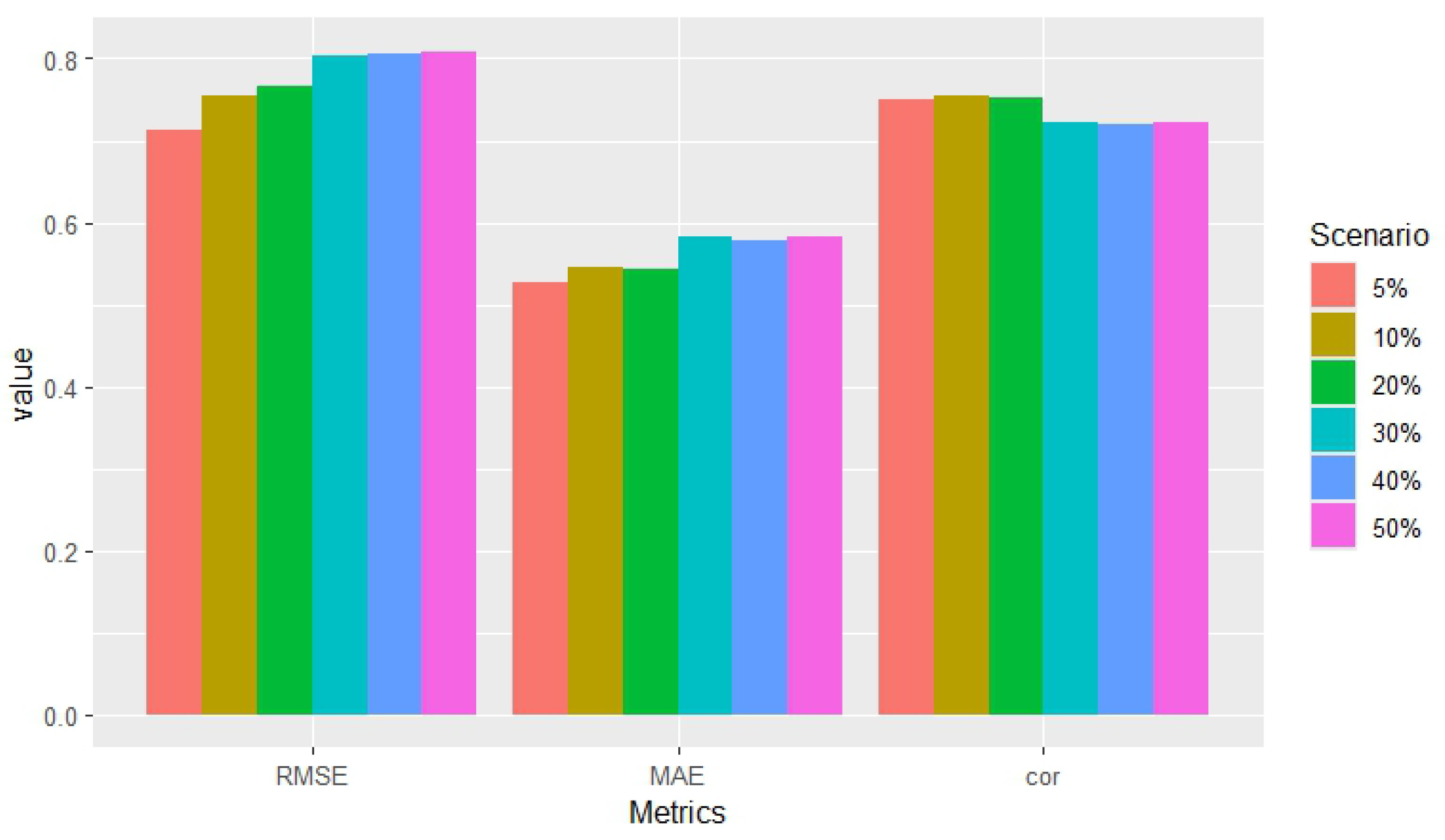
| Scenarios | RMSE | MAE | Correlation |
|---|---|---|---|
| 5% | 0.714 | 0.526 | 0.751 |
| 10% | 0.754 | 0.546 | 0.754 |
| 20% | 0.765 | 0.544 | 0.752 |
| 30% | 0.803 | 0.583 | 0.722 |
| 40% | 0.806 | 0.579 | 0.720 |
| 50% | 0.808 | 0.583 | 0.723 |
Disclaimer/Publisher’s Note: The statements, opinions and data contained in all publications are solely those of the individual author(s) and contributor(s) and not of MDPI and/or the editor(s). MDPI and/or the editor(s) disclaim responsibility for any injury to people or property resulting from any ideas, methods, instructions or products referred to in the content. |
© 2025 by the authors. Licensee MDPI, Basel, Switzerland. This article is an open access article distributed under the terms and conditions of the Creative Commons Attribution (CC BY) license (https://creativecommons.org/licenses/by/4.0/).
Share and Cite
Baena-Miret, S.; Reverter, F.; Sánchez, A.; Vegas, E. A Two-Step Algorithm for Handling Block-Wise Missing Data in Multi-Omics. Appl. Sci. 2025, 15, 3650. https://doi.org/10.3390/app15073650
Baena-Miret S, Reverter F, Sánchez A, Vegas E. A Two-Step Algorithm for Handling Block-Wise Missing Data in Multi-Omics. Applied Sciences. 2025; 15(7):3650. https://doi.org/10.3390/app15073650
Chicago/Turabian StyleBaena-Miret, Sergi, Ferran Reverter, Alex Sánchez, and Esteban Vegas. 2025. "A Two-Step Algorithm for Handling Block-Wise Missing Data in Multi-Omics" Applied Sciences 15, no. 7: 3650. https://doi.org/10.3390/app15073650
APA StyleBaena-Miret, S., Reverter, F., Sánchez, A., & Vegas, E. (2025). A Two-Step Algorithm for Handling Block-Wise Missing Data in Multi-Omics. Applied Sciences, 15(7), 3650. https://doi.org/10.3390/app15073650