Novel Real-Time Acoustic Power Estimation for Dynamic Thermoacoustic Control

Abstract

This paper presents a new procedure for the real-time processing and analysis of data from thermoacoustic systems. The approach focuses on continuously acquiring and adjusting measurements of acoustic wave pressure, enabling the instantaneous estimation of acoustic power. This is crucial for real-time control and decision-making, especially in applications that require rapid power estimation, such as the control loop implementation in thermoacoustic engines, where conditions are constantly changing and dynamic adaptation is essential. Two methods for estimating the power delivered to the load are proposed: (method 1) instantaneous power evaluation, which calculates the power consumed by the resistance in the resistance–capacitance (RC) load, and (method 2) one-period average power calculation using the well-established two-microphones method. These methods are validated with both different synthetic signals and experimental measurements. The results reveal that the new method provides real-time accurate estimations of the power delivered to the acoustic load and, thus, has shown potential for control-based applications.

1. Introduction

The thermoacoustic Stirling-like cycle engine (TA-SLiCE) represents an innovative class of external combustion engines designed to convert thermal energy into mechanical work and ultimately into direct current (DC) electrical energy [1]. These systems feature a thermoacoustic core with a regenerator between two heat exchangers, integrated into a looped acoustic network modelled as a lumped-element circuit due to its short-length component dimensions [2]. Over the years, the scientific community has extensively investigated the underlying thermoacoustic phenomena governing the operation of thermoacoustic engines, primarily aiming to improve the efficiency and performance of these systems [3]. Rott [4] established the fundamental theoretical framework for studying low-amplitude thermoacoustic phenomena under laminar flow conditions, providing the governing equations that describe the propagation of acoustic waves coupled with thermal effects in confined fluids. Later, Ceperley introduced the analogy between a traveling-wave thermoacoustic engine and a lumped-element electrical circuit [5], recognizing that the working fluid undergoes a thermodynamic cycle analogous to that of a Stirling engine [6]. This perspective facilitated the development of more efficient configurations and simplified the mathematical representation of these systems. More recently, Swift [7] refined and extended this approach through lumped-parameter models, providing more accessible and practical tools for the design and optimization of real thermoacoustic engines [8].

Thermoacoustic measurements often provide high signal-to-noise ratios, making the need for statistical analysis unnecessary [1]. While significant progress has been made in understanding the theoretical foundations and in optimizing the design of thermoacoustic engines [9,10], a variety of passive and active control strategies have been explored to improve the acoustic wave quality of these systems [11]. In this context, acoustic power is relatively easy to measure when volumetric velocity can be reliably inferred, with simpler techniques based on pressure measurements [12] or the motion of a solid object [13] being widely adopted in practice. More high-cost and sophisticated methods for direct velocity measurement, such as hot-wire anemometry particle, image velocimetry, or laser Doppler anemometry techniques, fall beyond the scope of this study and are covered in detail elsewhere [14]. The two-microphone measurement technique [15,16] is widely used to determine acoustic power from pressure amplitude and phase measurements at two locations in a resonator. This well-established method has been widely validated, particularly under laminar flow conditions, where it aligns with the analytical model developed by Fusco et al. [17], the so-called resistance–capacitance (RC) load method. These methodologies, supported by extensive and rigorous work [2], ensure reliable and robust power estimation across varying operational parameters (e.g., loads [18], temperatures, and pressures [19]), reinforcing the applicability of the proposed measurement framework to real-world thermoacoustic systems [20]. In all those studies, the measurement of acoustic power in thermoacoustic engines has been constrained by methods that rely on time-averaged estimations [21,22]. Although effective in many contexts, these methods do not account for potential fluctuations in acoustic amplitude within the mechanical resonator, which can reduce their effectiveness in applications such as control systems [23]. The ability to dynamically estimate acoustic power [24] and make immediate adjustments has been a long-standing challenge in thermoacoustic systems, where traditional optimization methods have typically relied on structural modifications [25] or temperature-based estimates [26]. Integrating real-time acoustic power measurements enables the system to respond to changes in performance as they occur, thereby ensuring more precise and adaptive control. Additionally, experimental constraints imposed by working within the low-amplitude regime required by linear theory, such as the subtle pressure oscillations, demand high-precision sensors or signal amplification lock-in systems [27], which significantly impact the cost and complexity of the data acquisition setup. In this context, recent studies have demonstrated that low-cost systems, such as those based on the Arduino platform, can achieve promising results in dynamic applications, ensuring reliability at reasonably high sampling rates when a reduced number of sensors are used [28]. The development of a robust yet affordable acquisition system requires optimizing sampling frequency, data transmission, and error mitigation, as demonstrated by Moreno [29], who enhanced acquisition rates and minimized errors in Arduino-based platforms. Building on these findings, this study utilizes the previously validated low-cost Arduino-based acquisition system designed for thermoacoustic Stirling engines [30]. This system has been optimized to reduce noise-related errors and enhance dynamic response, ensuring both accurate real-time thermoacoustic power estimation and reliable measurements.

This study presents a novel approach for the real-time estimation of instantaneous acoustic power in thermoacoustic engines, addressing the limitations of conventional time-averaged power estimation methods. The measurements are performed within a laminar regime, using the RC load-based method [30], where a resonator and a variable acoustic load are utilized to replicate the lossless acoustic behaviour of a piston in a linear alternator while accounting for parasitic losses due to piston motion. Unlike traditional methods that rely on time-averaged estimations, our procedure offers a way to measure instantaneous power by continuously acquiring and adjusting data on acoustic waves and system parameters. This allows real-time monitoring of the power dissipated in the RC load within the TA-SLiCE power extraction branch (see Figure 1), providing a more accurate and responsive approach for evaluating thermoacoustic power. Furthermore, the methodology is versatile and can be applied to various data acquisition systems, independent of their cost or complexity.

Figure 1. Illustration of the acoustic power visualization through a low-cost display.

The approach presented in this paper offers several advantages over traditional methods. A comparison between the real-time estimation technique and the widely used RC load-based method, which relies on averaged measurements, demonstrates that the proposed method provides accurate and timely results, even with a low-cost acquisition system. The effects of sampling rates and acquisition frequencies on measurement accuracy are also examined, showing that a higher resolution leads to reduced errors and greater precision in real-time applications. The obtained results emphasize the potential of real-time power measurement as a crucial tool for enhancing thermoacoustic engine performance, enabling new opportunities for control and optimization, such as the control algorithm developed by Callanan et al. [31], which improves efficiency and power density in thermoacoustic energy harvesters, making them more effective for practical applications in refrigeration and energy conversion.

The paper is organized as follows: In Section 2, the theoretical background and methodology for real-time power estimation in thermoacoustic engines is outlined. Section 3 describes the experimental setup, measurements, and results. Section 4 includes the experimental validation of the estimation procedure, comparison with traditional approaches, and discussion. Section 5 provides the main conclusions of this work.

2. Materials and Methods

In this section, the analogy between different acoustic and electrical magnitudes will be presented, which will allow the development of an equivalent electrical model. From this model, it will be possible to calculate the electrical power consumed and, by analogy of the models, to estimate the acoustic power provided by the engine. On the other hand, different acoustic power measurement methods will be explored, both for the calculation of the average value and for its measurement in real time, and various comparisons will be made between these methods, including the RC load method, which is firmly established.

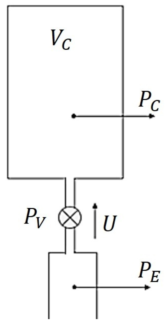
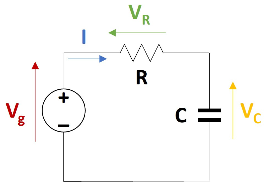
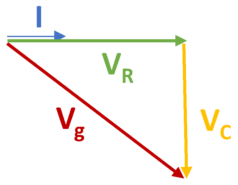
2.1. RC Equivalent Model in Electrical Analogy

The acoustic wave interactions in thermoacoustic devices are difficult to analyse, either because of their physical complexity or because of their dependence on the medium in which the wave propagates, in many cases requiring the use of very advanced tools. It is possible to establish an electric-acoustic correspondence thanks to the similarity of the fundamental equations that govern both disciplines [1,32]. The analogies relevant to this article are shown in Table 1. This similarity enables the representation of complex acoustic systems as simplified electrical circuits, facilitating the use of electrical analysis tools and simulators for efficient system evaluation and optimization.

Table 1. Electro-Acoustic analogous variables.

Physical Variable	Electrical Analogy
Acoustic pressure (P)	Electrical voltage (V)
Volume flow rate (U)	Current (I)
Resistance (R)	Resistance (R)
Compliance (C)	Capacitance (C)
$\mathrm{Acoustic} \mathrm{power} \left({\dot{E}}_{load}\right)$	Electric power (Pelec)

The acoustic RC load in the power extraction branch of a TA-SLiCE, depicted in Figure 2, consists of a small tank of volume $V_C$ (compliance) connected through a needle valve to the mechanical branch resonator.

Figure 2. Diagram of a thermoacoustic resistance–capacitance (RC) load. $P_C$, $P_E$, and $P_V$ are the pressures at the compliance, the resonator, and the valve, respectively. $U$ is the volume flow rate through the valve.

The expression describing the process is given by Equation (1):

$$P_E\left(t\right)=P_V\left(t\right)+P_C\left(t\right),$$

(1)

According to the electro-acoustic analogies shown in the table above and the physical problem under consideration, the pressure in the resonator, $P_E\left(t\right)$, is analogous to the total voltage or source voltage, $V_g\left(t\right)$. Similarly, the pressure in the capacitor $P_C\left(t\right)$ corresponds to the capacitor voltage $V_C\left(t\right)$ and the pressure in the valve, $P_V\left(t\right)$, is analogous to the resistor voltage $V_g\left(t\right)$. On the other hand, the analogue to the volume flow rate, $U\left(t\right)$, is the circuit current, $I\left(t\right)$. This results in Equation (2) and the corresponding electrical model shown in Figure 3.

$$V_g\left(t\right)=V_R\left(t\right)+V_C\left(t\right),$$

(2)

Figure 3. Electric RC load, where V_C, V_g, and V_R are the voltages at the capacitor, the source, and the resistor and I is the current though the circuit.

On the other hand, the characteristic equation of a capacitor is

$$i_C\left(t\right)=C{\displaystyle \frac{d{V}_C\left(t\right)}{dt}} ,$$

(3)

where $C$ is the capacitance of the capacitor and $i_C\left(t\right)$ is the current flowing through it. As the elements are in series, the current flowing through the whole circuit would be the same:

$$I\left(t\right)=i_C\left(t\right)=C{\displaystyle \frac{d{V}_C\left(t\right)}{dt}},$$

(4)

If the circuit analysis is performed in steady state, phasor notation can be used, leading to

$$\overrightarrow{V_g}=\overrightarrow{V_R}+\overrightarrow{V_C},$$

(5)

where $\overrightarrow{V_g}$, $\overrightarrow{V_R}$, and $\overrightarrow{V_C}$ are the voltage phasors of the source, the resistor, and the capacitor, respectively.

$$\overrightarrow{I}=jwC\overrightarrow{V_C},$$

(6)

The $\overrightarrow{I}$ denotes the current phasor. The capacitor voltage, as a function of the current flowing through it, is expressed in Equation (7):

$$\overrightarrow{V_C}={\displaystyle \frac{1}{jwC}}\overrightarrow{I}=-{\displaystyle \frac{j}{wC}}\overrightarrow{I},$$

(7)

The phasor of a number in polar form is expressed by its magnitude and phase, such that $\overrightarrow{I}=I\angle {\phi }_I$, $\overrightarrow{V_R}=V_R\angle {\phi }_{VR}$, and $\overrightarrow{V_C}=V_C\angle {\phi }_{VC}$ are the phasors, expressed in polar form, of the current, the voltage across the resistor, and the voltage across the capacitor, respectively. As the circuit is in series, considering the current as the phase reference, $\overrightarrow{I}=I\angle 0°$ the voltage at the terminals of the resistor will be in phase with the current passing through it, $\overrightarrow{V_R}=V_R\angle 0$ and the voltage at the capacitor will be delayed by $90°$ with respect to the same current, $\overrightarrow{V_C}=V_C\angle -90°$ as illustrated in the phasor diagram in Figure 4.

Figure 4. Phasor diagram of an RC load.

2.2. Average Power Estimation

The RC load method has been widely adopted as a reliable approach for measuring acoustic power in thermoacoustic systems [17]. This method utilizes the phasor representation of the volumetric flow rate across the resistance, derived from the pressure oscillations within the compliance, $C$, assuming the short duct length approximation:

$$U=j\omega C{P}_C=j\omega {\displaystyle \frac{V}{\gamma P_m}} P_C,$$

(8)

where $U$ represents the volumetric flow rate, $P_C$ the pressure measured at the compliance and V, $P_m$, and $\gamma$ correspond to the compliance volume, mean pressure, and specific heat ratio, respectively [1].

Using this relationship, the dissipated acoustic power at the resistance is determined by analysing the two key pressure signals, $P_C$ and $P_E$, in terms of their amplitude, phase, and angular frequency:

$${\dot{E}}_{load}={\displaystyle \frac{1}{2}}{\displaystyle \frac{\omega V}{\gamma P_m}}Im\left(P_E{\tilde{P}}_C\right)={\displaystyle \frac{1}{2}}{\displaystyle \frac{\omega V}{\gamma P_m}}\left|P_E\right|\left|P_C\right|sin{\theta }_{EC},$$

(9)

where ${\theta }_{EC}$ is the phase angle between the $P_C$ and $P_E$ pressure signals. The short duct length approximation allows this method to be consistently expressed in terms of the compliance of geometric and thermodynamic parameters [33].

The RC load method determines the dissipated acoustic power as the time-averaged product of the volumetric flow rate through the valve and the pressures $P_C$ and $P_E$ across it [30].

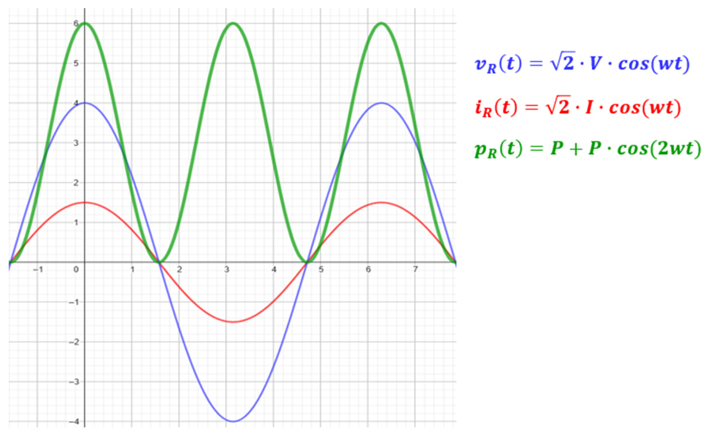
2.3. Instantaneous Power Estimation

By measuring the pressure difference in the resonator and in the small tank, it will be possible to determine the acoustic power lost, ${\dot{E}}_{load}$, by simply multiplying this difference by the flow rate through the valve.

$${\dot{E}}_{load}=P_V·U=(P_E-P_C)·U,$$

(10)

where $P_V$ is the pressure in the valve.

Using the electro-acoustic analogy to the electrical power equation would leave

$${\dot{E}}_{load}=P_{elec}=V_R·I=\left(V_g-V_C\right)·I,$$

(11)

To calculate the power at each time instant, the following expression for the instantaneous power $P_{elec}\left(t\right)$ is employed:

$$P_{elec}\left(t\right)=V_R\left(t\right)·I\left(t\right)=\left(V_g\left(\mathrm{t}\right)-V_C\left(t\right)\right)·I\left(t\right)=\left(V_g\left(\mathrm{t}\right)-V_C\left(t\right)\right)·C{\displaystyle \frac{d{V}_C\left(t\right)}{dt}},$$

(12)

where $V_R\left(t\right), V_g\left(t\right)$, and $V_C\left(t\right)$ are the instantaneous voltages across the resistor, the source, and the capacitor, respectively, and $I\left(t\right)$ is the instantaneous current flowing through the circuit. Under the assumption of a short duct length, the expression for the electrical power is derived as

$$P_{elec}\left(t\right)={\displaystyle \frac{V}{\gamma P_m}}·\left(V_g\left(t\right)-V_C\left(t\right)\right)·{\displaystyle \frac{d{V}_C\left(t\right)}{dt}},$$

(13)

Applying the electro-acoustic analogy to the acoustic power equation would leave

$${\dot{E}}_{load}\left(t\right)={\displaystyle \frac{V}{\gamma P_m}}·(P_E\left(t\right)-P_C\left(t\right))·{\displaystyle \frac{d{P}_C\left(t\right)}{dt}} ,$$

(14)

The instantaneous power in any element of an alternating current circuit is expressed as $p\left(t\right)=v\left(t\right)·i\left(t\right)$, where v(t) and i(t) represent the voltage and current at each moment, respectively. If the source supplying the circuit produces a sinusoidal alternating current, both the voltage and current of each element will be represented by sinusoidal waves. These waves will exhibit a relative phase shift, determined by the specific characteristics of the element where the instantaneous power is being evaluated.

The expression for instantaneous power, $P_{elec}\left(t\right)$, as a function of the voltage and current of an element of an electrical circuit is defined as

$$P_{elec}\left(t\right)=v\left(t\right)·i\left(t\right)=2·V·I·\cos \left(w·t\right)\cos \left(w·t-\phi \right),$$

(15)

where V and I represent the root mean square (RMS) voltage and current of that element. $w$ represents the angular frequency and $\phi$ is the phase angle between the voltage and the current of the element.

By applying the trigonometric identities for sine and cosine of a double angle, this expression can be reformulated, as follows:

$$P_{elec}\left(t\right)=P·\left(1+\cos \left(2·w·t\right)\right)+Q·sen\left(2·w·t\right),$$

(16)

where P and Q are the active and reactive power, respectively, consumed by the passive element.

The average value of this instantaneous power is the active power, P, the power that provides the energy that is converted into effective or useful work, either in the form of heat, light, or motion.

$$\overline{P_{elec}\left(t\right)}=P,$$

(17)

In this case, the instantaneous power to be measured and calculated is that of the resistive element of the circuit, where the voltage at the terminals of the resistor and the current flowing through it are in phase. Figure 5 shows a singular case of the voltage and current in a resistive element, as well as the instantaneous power.

Figure 5. Voltage, current, and instantaneous power in a resistive element.

3. Results

The acoustic power measurement system described in this paper has two main components: (i) the real-time data-acquisition system that measures the pressure both in the compliance ($P_C$) and the resonator ($P_E$) and (ii) the data-processing system, which scales and filters the measurements (Section 3.1) and then calculates the power delivered to the load (Section 3.2 and Section 3.3).

The former, which builds upon a thoroughly validated setup, described in previous research [30], is based on an Arduino platform designed to accurately calculate the acoustic power of the TA-SLiCE. In that earlier work, the performance of this setup was shown to be both reliable and accurate, confirming its suitability for measuring acoustic power in thermoacoustic engines. Integrated with piezoelectric low-cost pressure sensors, the system enables the real-time measurement and transmission of sensor data, ensuring continuous monitoring of pressure variations in two key components of the system: the compliance, which functions as a dynamic capacitor, and the resonator, responsible for the acoustic oscillations.

The latter is described in this section of the paper. Two different approaches for estimating the power delivered to the load are proposed:

• Instantaneous power evaluation (method 1), which consists of using the instantaneous power consumed in the resistance of the equivalent RC model of the load;
• One-period average power calculation (method 2), in which the procedure established by Fusco et al. [17] is adapted to be used each single period for each single period of the signal.

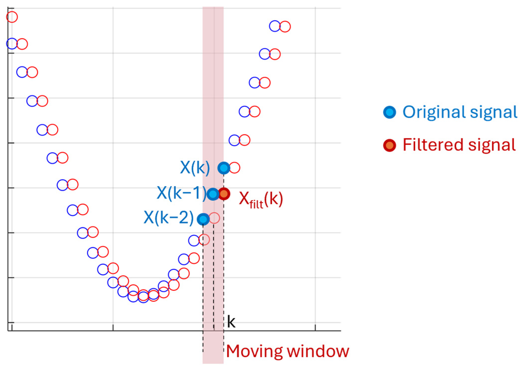
3.1. Measurements Conditioning

The data-acquisition system described in [30] provides pressure measurements that are already expressed in mbar. However, the following steps are needed prior to the calculation of the power delivered to the load.

First, the acoustic pressure wave and the average pressure value need to be split up. Alternatively, expressing this idea with electrical terms, the alternating current (AC) wave and the DC operation point need to be separated. To do so, the DC component of cycle c is calculated based on the maximum and minimum values of the signal in cycle c − 1:

$$X_{DC}\left(c\right)={\displaystyle \frac{X_{max}\left(c-1\right)+X_{min}\left(c-1\right)}{2}},$$

(18)

where $X_{DC}\left(c\right)$ refers to the DC component of signal X in cycle c, whereas $X_{max}\left(c-1\right)$ and $X_{min}\left(c-1\right)$ are the maximum and minimum values of the signal X in cycle c − 1, respectively (see Figure 6).

Figure 6. Estimation of the average value of the signal based on the previous cycle.

This procedure is simple and provide a good estimation of the DC component of the signal, but it cannot be used to calculate the DC component of the first cycle. Therefore, the following expression is used to calculate the DC component for each time step k:

$$X_{DC}\left(k\right)={\displaystyle \frac{{\sum }_{j=1}^{k}X\left(j\right)}{k}},$$

(19)

where $X_{DC}\left(k\right)$ and $X\left(k\right)$ refer to the DC component and the value of signal X in time step k, respectively.

Figure 7 shows the response of the DC component estimation algorithms in the initial cycle (see Equation (19)) and the rest of the cycles (see Equation (18)).

Figure 7. Estimation of the average value of the signal based on the first cycle.

Once the AC and DC components have been split up, the AC signal is filtered to reduce the noise using a moving average:

$$X_{filt}\left(k\right)={\displaystyle \frac{{\sum }_{j=0}^{W-1}X\left(k-j\right)}{W}},$$

(20)

where $X_{filt}\left(k\right)$ is the filtered value of the signal and W is the size of the moving window.

As shown in Figure 8, this filtering technique causes some delay in the filtered signal compared to the original one and, therefore, the size of the moving windows needs to be selected as a trade-off between the noise reduction and the admissible delay.

Figure 8. Moving-average-based filtering of the drawing, with W = 3.

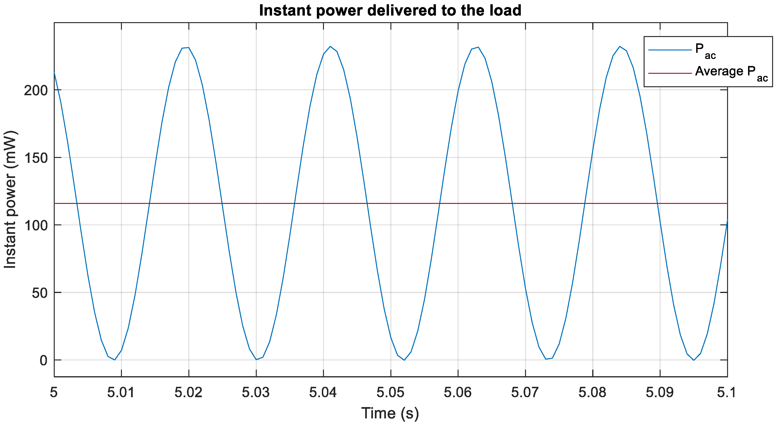
3.2. Instantaneous Power Calculation by Method 1

In this section, the instantaneous power calculation by method 1 is presented, relying on Equation (8) to evaluate the power consumed by the resistance of the RC load at each time lapse.

The derivative of $P_C\left(t\right)$ for a given time step k can be approximated as follows:

$${\displaystyle \frac{d{P}_C\left(k\right)}{dt}}\approx {\displaystyle \frac{P_{C,filt}\left(k\right)-P_{C,filt}\left(k-1\right)}{T_S}},$$

(21)

where $T_S$ is the sampling period and $P_{C,filt}\left(k\right)$ is the filtered value of the pressure at the compliance at time step k.

Therefore, the power delivered to the load at a time step k can be expressed as

$${\dot{E}}_{load}\left(k\right)={\displaystyle \frac{V}{\gamma P_m}}·\left(P_{E,filt}\left(k\right)-P_{C,filt}\left(k\right)\right)·{\displaystyle \frac{P_{C,filt}\left(k\right)-P_{C,filt}\left(k-1\right)}{T_S}},$$

(22)

where $P_{E,filt}\left(k\right)$ is the filtered value of the pressure in the resonator at time step k.

To determine the average value of the power delivered to the load, the following expression can be used:

$$\overline{{\dot{E}}_{load,method1}}={\displaystyle \frac{{\sum }_{j=1}^{N_S}{P}_{ac}\left(j\right)}{N_S}},$$

(23)

where $N_S$ is the number of samples considered for averaging.

According to Equation (17), the average value of $P_{ac}\left(t\right)$ can alternatively also be calculated as

$$\overline{{\dot{E}}_{load,method1}}={\displaystyle \frac{{\dot{E}}_{load,max}}{2}},$$

(24)

where ${\dot{E}}_{load,max}$ is the maximum value of ${\dot{E}}_{load}\left(k\right)$.

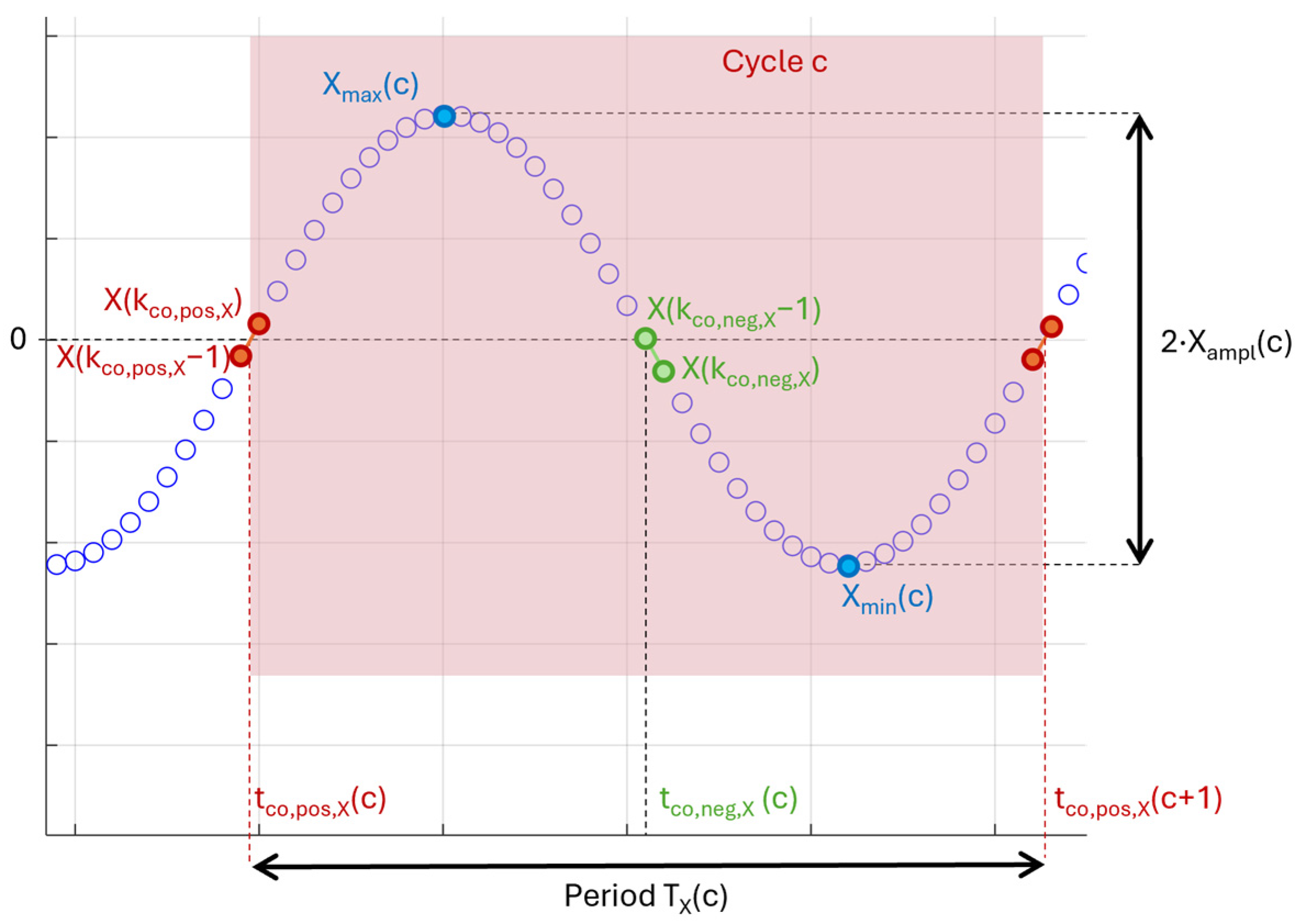
3.3. One-Period Average Power Calculation by Method 2

The one-period average power calculation (method 2) uses Equation (22) to calculate the average power delivered to the load but, instead of determining $P_E$, $P_C$, and ${\theta }_{EC}$ over a large number of periods by means of the Fast Fourier Transform (FFT) and least-squares fitting, they are obtained by identification over a single period (see Figure 9).

Figure 9. Identification of relevant quantities of the signal for method.

Given a signal X(k), the maximum and minimum values measured in a cycle c (referred to as $X_{max}\left(c\right)$ and $X_{min}\left(c\right)$, respectively) are used to calculate the amplitude $X_{ampl}\left(c\right)$ of the signal:

$$X_{ampl}\left(c\right)={\displaystyle \frac{X_{max}\left(c\right)-X_{min}\left(c\right)}{2}},$$

(25)

For a cycle c, the crossover time with a positive slope $t_{co,pos,X}\left(c\right)$ is obtained by (i) detecting the time step $k_{co,pos,X}$ at which the signal X becomes positive after being negative and (ii) conducting a linear interpolation to determine $t_{co,pos,X}\left(c\right)$ at which X(t) equals 0. If needed, the crossover time with a negative slope $t_{co,neg}\left(c\right)$ can also be determined by detecting the time step $k_{co,neg.X}$ at which the signal X becomes negative after being positive.

The period $T_X\left(c\right)$ of a signal X can then be calculated as

$$T_X\left(c\right)=t_{co,pos,X}\left(c\right)-t_{co,pos,X}\left(c-1\right),$$

(26)

The acquisition system just described allows to measure this expression and can also be reformulated in terms of the active and reactive power consumed by the element, as follows:

$${\dot{E}}_{load}\left(c\right)={\displaystyle \frac{1}{2}}{\displaystyle \frac{\omega V}{\gamma P_m}}{P}_E\left(c\right)·P_C\left(c\right)·sin{\theta }_{EC}\left(c\right),$$

(27)

where $P_E\left(c\right)$ is the amplitude of $P_{E,filt}\left(k\right)$ in cycle c, $P_C\left(c\right)$ is the amplitude of $P_{C,filt}\left(k\right)$ in cycle c, and ${\theta }_{EC}\left(c\right)$ is the phase difference between $P_{E,filt}$ and $P_{C,filt}$.

The phase difference ${\theta }_{EC}\left(c\right)$, expressed in radians, can be calculated as

$${\theta }_{EC}\left(c\right)={\displaystyle \frac{2\pi }{T_{PE}\left(c\right)}} \left(t_{co,pos,Pc}\left(c\right)-t_{co,pos,Pe}\left(c\right)\right),$$

(28)

where $T_{PE}\left(c\right)$ is the period of $P_{E,filt}\left(k\right)$ in cycle c, $t_{co,pos,Pc}\left(c\right)$ is the crossover time with a positive slope of $P_{C,filt}$ in cycle c, and $t_{co,pos,Pe}\left(c\right)$ is the crossover time with a positive slope of $P_{E,filt}$ in cycle c.

4. Discussion

To evaluate the accuracy of the proposed methods, the following studies are carried out:

• First, simulated values of $P_E\left(k\right)$ and $P_C\left(k\right)$ with no noise and a good sampling frequency are considered. The average power delivered to the load is calculated using the proposed methods and compared to the results obtained with the reference procedure [17].
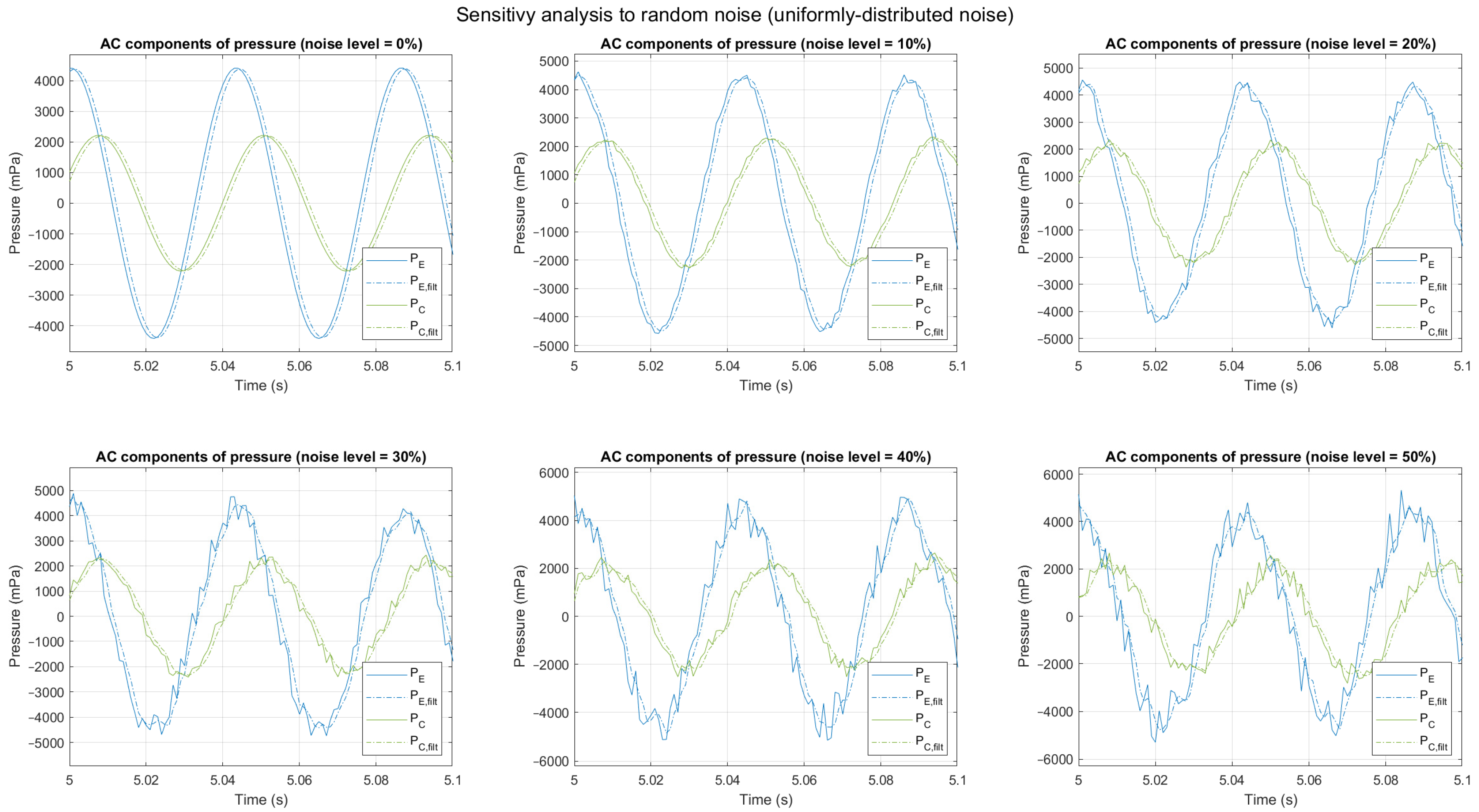
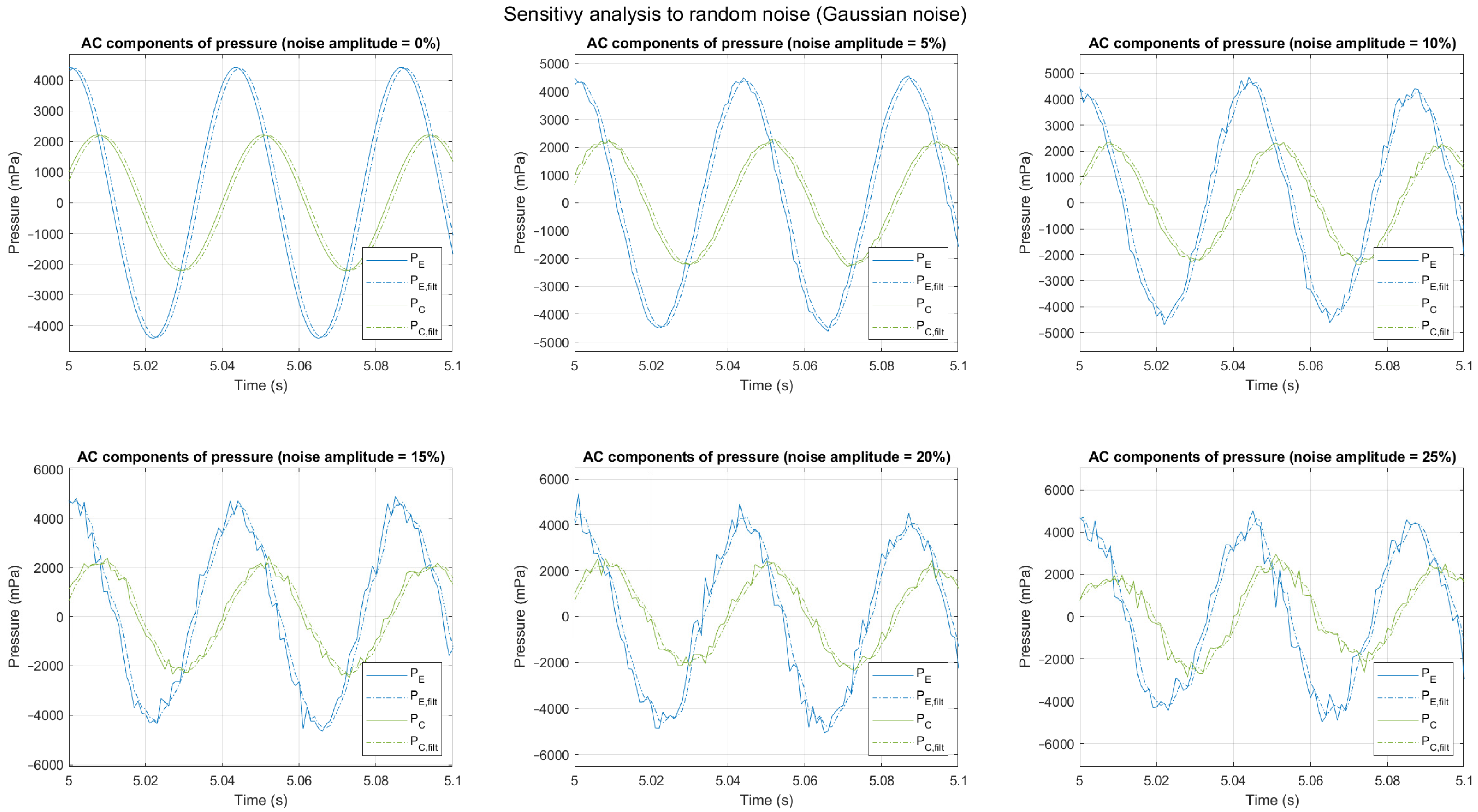
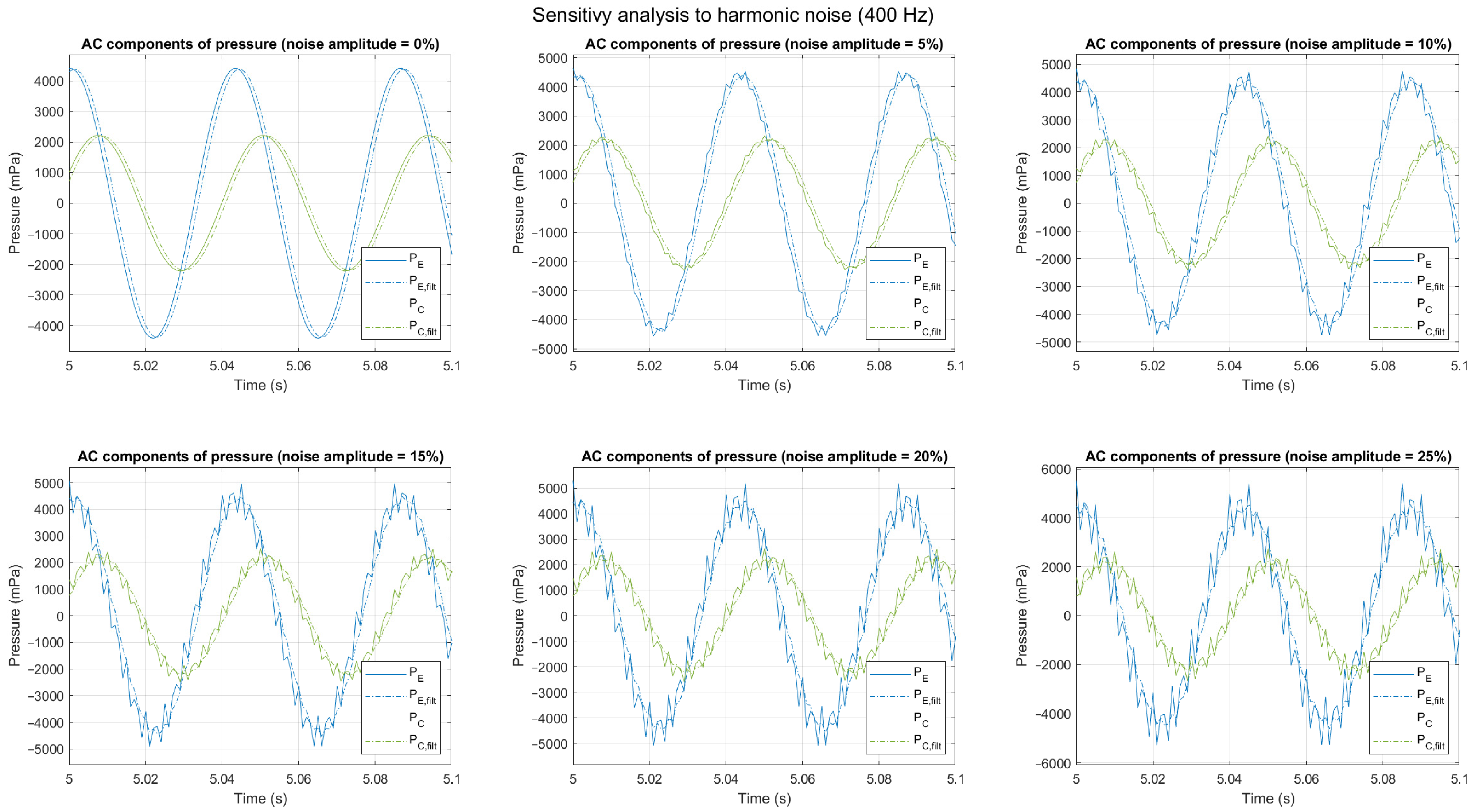
• Then, the sensitivity to the noise is analysed, for which a random noise is added to the simulated of $P_E\left(k\right)$ and $P_C\left(k\right)$;
• Afterwards, the sensitivity to the measurement frequency is analysed, for which the sampling frequency of $P_E\left(k\right)$ and $P_C\left(k\right)$ is reduced;
• Finally, real measurements of $P_E\left(k\right)$ and $P_C\left(k\right)$ are used to conduct the analysis.

4.1. Results Using Ideal Signals

For this analysis, the following functions $P_E\left(\mathrm{t}\right)$ and $P_C\left(\mathrm{t}\right)$ were considered over the interval from 0 to 10 s, with a sampling time of 1 ms:

$$P_E\left(\mathrm{t}\right)=78309+4421.3·\cos \left(145.76·\mathrm{t}\right),$$

(29)

and

$$P_C\left(\mathrm{t}\right)=78359+2218.7·\cos \left(145.76·\mathrm{t}-1.0451\right),$$

(30)

Figure 10 shows the convergence of the DC component estimation for both $P_E\left(\mathrm{t}\right)$ and $P_C\left(\mathrm{t}\right)$. The DC component estimation algorithm shows good convergence, stabilizing after approximately three cycles.

Figure 10. Estimation of the direct current (DC) component of the signal of $P_E\left(k\right)$ and $P_C\left(k\right)$ (ideal signals).

Figure 11 compares the AC component of $P_E\left(\mathrm{t}\right)$ and $P_C\left(\mathrm{t}\right)$, both filtered and non-filtered. The moving window size for the filtering is W = 3 in all the study cases.

Figure 11. Alternating current (AC) component of $P_E\left(k\right)$ and $P_C\left(k\right)$ analyzed for ideal signals, considering both non-filtered and filtered cases.

Figure 12 shows the instantaneous power obtained using method 1.

Figure 12. Instantaneous power obtained using Equation (22) for ideal signals.

Table 2 shows the average power obtained with the proposed methods and compares them to the average power obtained with the reference procedure [17]. The error is defined as follows:

$$Error\left(\%\right)={\displaystyle \frac{{\dot{E}}_{load,ref}-{\dot{E}}_{load,method}}{{\dot{E}}_{load,ref}}}·100,$$

(31)

where ${\dot{E}}_{load,ref}$ is the average power obtained with the reference procedure and ${\dot{E}}_{load,method}$ refers to the average power obtained with the proposed methods (1 or 2).

Table 2. Comparison of the results obtained using different methods (ideal signals).

Method	Average Power (mW)	Error (%)
Reference method	118.05	--
Instantaneous power (method 1)	115.97	1.75
One-period average (method 2)	116.69	1.15

The first three cycles (needed to stabilize the DC components) have not been considered in calculating the averages.

These results show that good correspondence is obtained when using the three methods with an ideal synthesis signal sampled at approximately 40 measurements per period: the difference is lower than 1.8%.

4.2. Sensitivity to Noise

For this analysis, the following functions $P_E\left(\mathrm{t}\right)$ and $P_C\left(\mathrm{t}\right)$ have been considered in the interval between 0 a 10 s (sampling time is 1 ms):

$$P_E\left(\mathrm{t}\right)=78309+4421.3·\left(\cos \left(145.76·\mathrm{t}\right)+\mathrm{NoiseLevel}·\mathrm{Noise}()\right),$$

(32)

and

$$P_C\left(\mathrm{t}\right)=78359+2218.7·\left(\cos \left(145.76·\mathrm{t}-1.0451\right)+\mathrm{NoiseLevel}·\mathrm{Noise}()\right),$$

(33)

where NoiseLevel is the amplitude of the noise expressed in per unit and Noise() is a noise function which will vary depending on the type of noise to be analysed.

4.2.1. Uniformly-Distributed Random Noise

In this case, Noise() is a function which follows a uniform distribution from −1 to 1. Figure 13 represents the functions $P_E\left(\mathrm{t}\right)$ and $P_C\left(\mathrm{t}\right)$ obtained using Equations (32) and (33) with different noise levels.

Figure 13. AC component of $P_E\left(k\right)$ and $P_C\left(k\right)$, filtered and non-filtered, with different noise levels (uniformly distributed noise).

Table 3 shows how adding a uniformly-distributed noise to $P_E\left(\mathrm{t}\right)$ and $P_C\left(\mathrm{t}\right)$ impacts into the calculated power depending on the method.

Table 3. Comparison of the results obtained with different levels of noise (uniformly distributed noise).

Method	Average Power (mW) for Different Levels of Noise (Uniformly Distributed Noise)
	0%	5%	10%	15%	20%	25%
Reference method	118.05	117.969	118.377	117.987	118.310	117.931
Instantaneous power (method 1)	115.983	115.814	115.788	115.216	114.332	113.789
One-period average (method 2)	116.691	117.355	119.879	122.161	126.007	128.734

The results of this analysis show some degradation of the accuracy of the result when noise increases. When the noise level is 25%, the average power obtained is 113.789 mW (which corresponds to an error of 3.5%) and 128.734 mW (which corresponds to an error of −9.2%) using methods 1 and 2, respectively. In general, method 1 tends to underestimate the average power, whereas method 2 tends to overestimate it.

Although method 2 has shown better accuracy with lower noise levels, method 1 has shown better robustness when noise increases. This is mainly because method 2 relies on the peak values of the filtered signals, which are more sensitive to the noise, to determine the averaged power.

4.2.2. Gaussian Random Noise

In this case, Noise() is a function which follows a Gaussian distribution with a mean of 0 and standard deviation of 1. Since the Gaussian noise is not mathematically bounded, the amplitude of the noise has been assumed to be equal to two times the standard deviation (which is a bound for 95.4% of the possible values). Figure 14 represents the functions $P_E\left(\mathrm{t}\right)$ and $P_C\left(\mathrm{t}\right)$ obtained using Equations (32) and (33) with different noise levels.

Figure 14. AC component of $P_E\left(k\right)$ and $P_C\left(k\right)$, filtered and non-filtered, with different noise levels (gaussian noise).

Table 4 shows how adding a gaussian noise to $P_E\left(\mathrm{t}\right)$ and $P_C\left(\mathrm{t}\right)$ impacts into the calculated power depending on the method.

Table 4. Comparison of the results obtained with different levels of noise (Gaussian noise).

Method	Average Power (mW) for Different Levels of Noise (Gaussian Noise)
	0%	5%	10%	15%	20%	25%
Reference method	118.05	117.924	118.086	117.418	118.265	117.952
Instantaneous power (method 1)	115.983	115.817	115.665	115.065	115.022	114.140
One-period average (method 2)	116.691	117.288	119.136	121.281	124.101	126.584

The results of this analysis show a degradation of the accuracy of the result when noise increases. When the noise level is 15%, the average power obtained is 114.140 mW (which corresponds to an error of 3.2%) and 126.584 mW (which corresponds to an error of −7.3%) using methods 1 and 2, respectively. In general, method 1 tends to underestimate the average power, whereas method 2 tends to overestimate it. As observed with uniformly distributed noise, method 1 has shown better robustness when noise increases.

4.2.3. Harmonic Noise

In this case, Noise() is a cosine function with a given frequency (for this analysis, a noise frequency of 400 Hz has been considered, a frequency one decade larger than the measured signals). Figure 15 represents the functions $P_E\left(\mathrm{t}\right)$ and $P_C\left(\mathrm{t}\right)$ obtained using Equations (32) and (33) with different noise levels.

Figure 15. AC component of $P_E\left(k\right)$ and $P_C\left(k\right)$, filtered and non-filtered, with different noise levels (harmonic noise, 400 Hz).

Table 5 shows how adding a gaussian noise to $P_E\left(\mathrm{t}\right)$ and $P_C\left(\mathrm{t}\right)$ impacts into the calculated power depending on the method.

Table 5. Comparison of the results obtained with different levels of noise (harmonic noise, 400 Hz).

Method	Average Power (mW) for Different Levels of Noise (Harmonic Noise, 400 Hz)
	0%	5%	10%	15%	20%	25%
Reference method	118.05	118.052	118.053	118.054	118.055	118.056
Instantaneous power (method 1)	115.983	116.015	116.281	116.727	117.351	118.155
One-period average (method 2)	116.691	117.751	119.426	121.266	123.170	125.137

The results of this analysis show a degradation of the accuracy of the result when noise increases. When the noise level is 15%, the average power obtained is 118.155 mW (which corresponds to an error of −0.08%) and 125.137 mW (which corresponds to an error of −6%) using methods 1 and 2, respectively. As observed with uniformly distributed noise, method 1 has shown better robustness when noise increases.

4.3. Sensitivity to the Sampling Frequency

For this analysis, the functions $P_E\left(\mathrm{t}\right)$ and $P_C\left(\mathrm{t}\right)$ have been used as in Equations (29) and (30), but the sampling time is swept between 0.1 ms and 5 ms. As a reference, both $P_E\left(\mathrm{t}\right)$ and $P_C\left(\mathrm{t}\right)$ have a period equal to 43.1 ms.

Figure 16 represents the functions $P_E\left(\mathrm{t}\right)$ and $P_C\left(\mathrm{t}\right)$ obtained using Equations (32) and (33) with different sampling periods from 0.5 ms to 5 ms. In the latter, the piecewise aspect can easily be observed.

Figure 16. AC component of $P_E\left(k\right)$ and $P_C\left(k\right)$, filtered and non-filtered, with different sampling periods.

Table 6 shows how the sampling time impacts in the average power calculated using the proposed methods.

Table 6. Comparison of the results obtained with different sampling times.

Method	Average Power (mW) for Different Sampling Periods Ts
	0.1 ms	0.5 ms	1 ms	2 ms	3 ms	4 ms	5 ms
Reference method	118.050	118.050	118.050	118.050	118.050	118.050	118.050
Instantaneous power (method 1)	118.025	117.530	115.983	109.957	100.417	88.3360	74.2730
One-period average (method 2)	118.551	118.097	116.691	111.200	102.506	91.3430	77.9310

These results show that the estimation error observed when using ideal synthesis signals of $P_E\left(\mathrm{t}\right)$ and $P_C\left(\mathrm{t}\right)$ (see Table 2) is partially due to the sampling frequency. In fact, a noticeable degradation of the results (more than 10%) has been remarked when the number of measurements falls under 15 samples per cycle of the signal (i.e., with sampling time is longer than 3 ms).

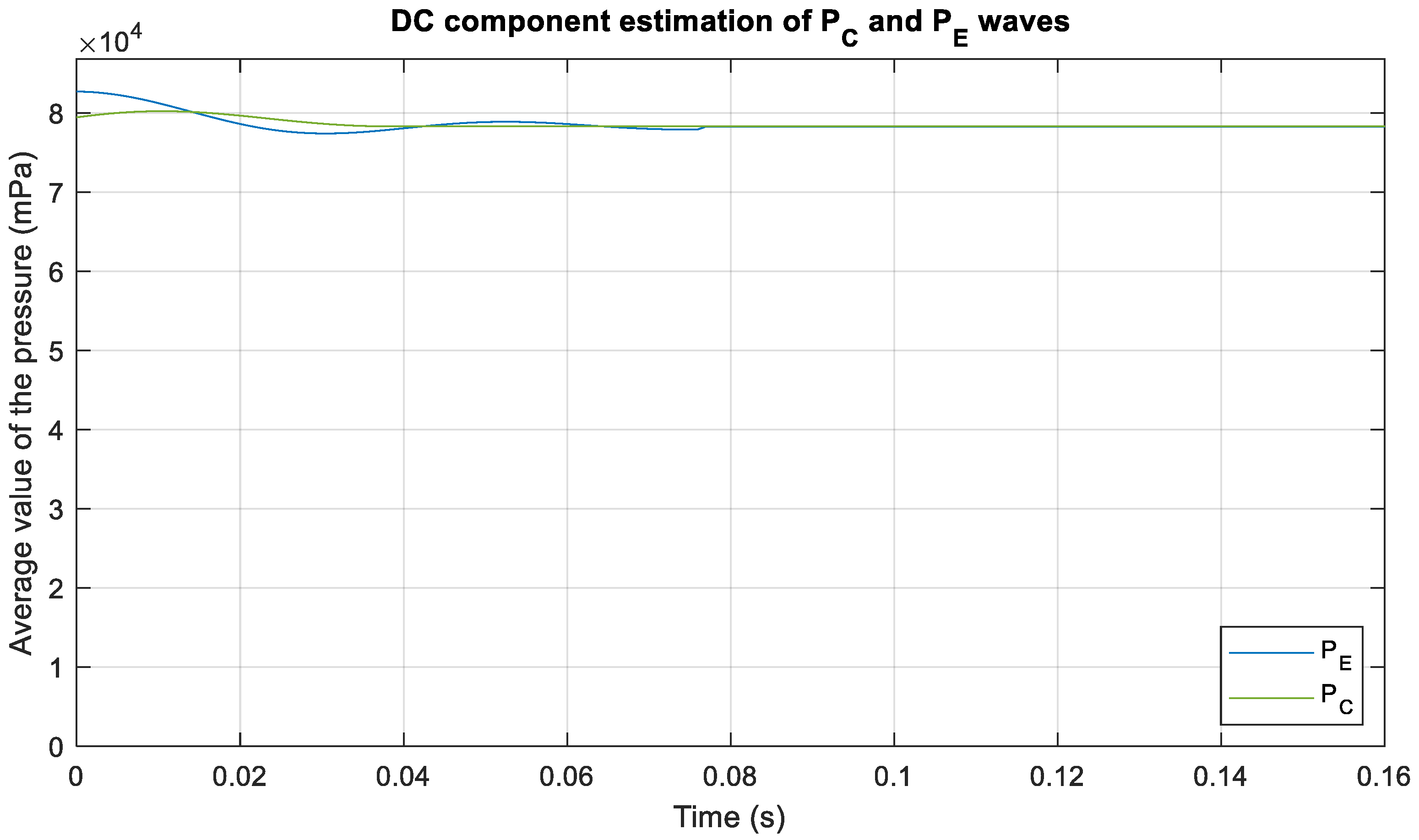
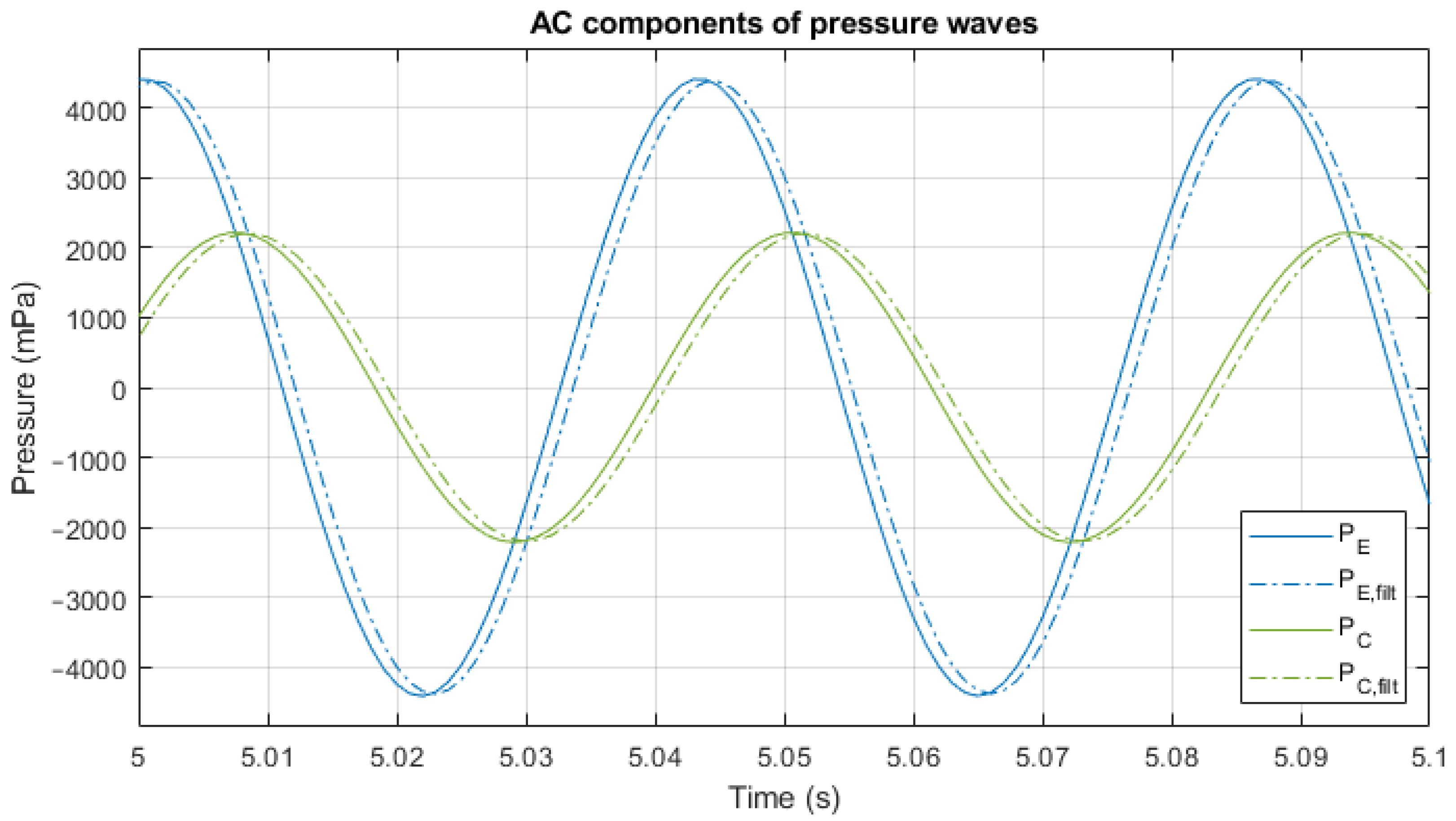
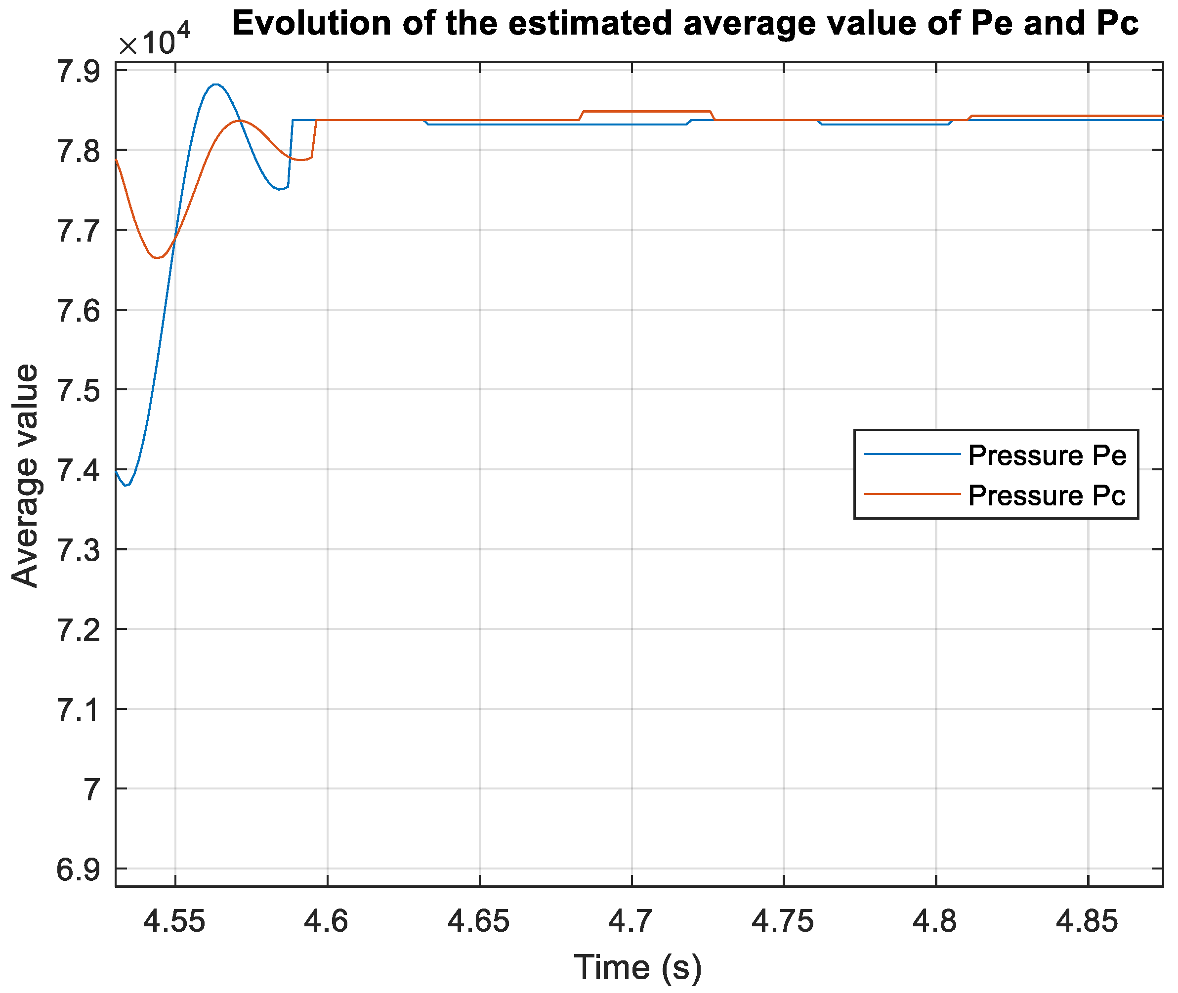
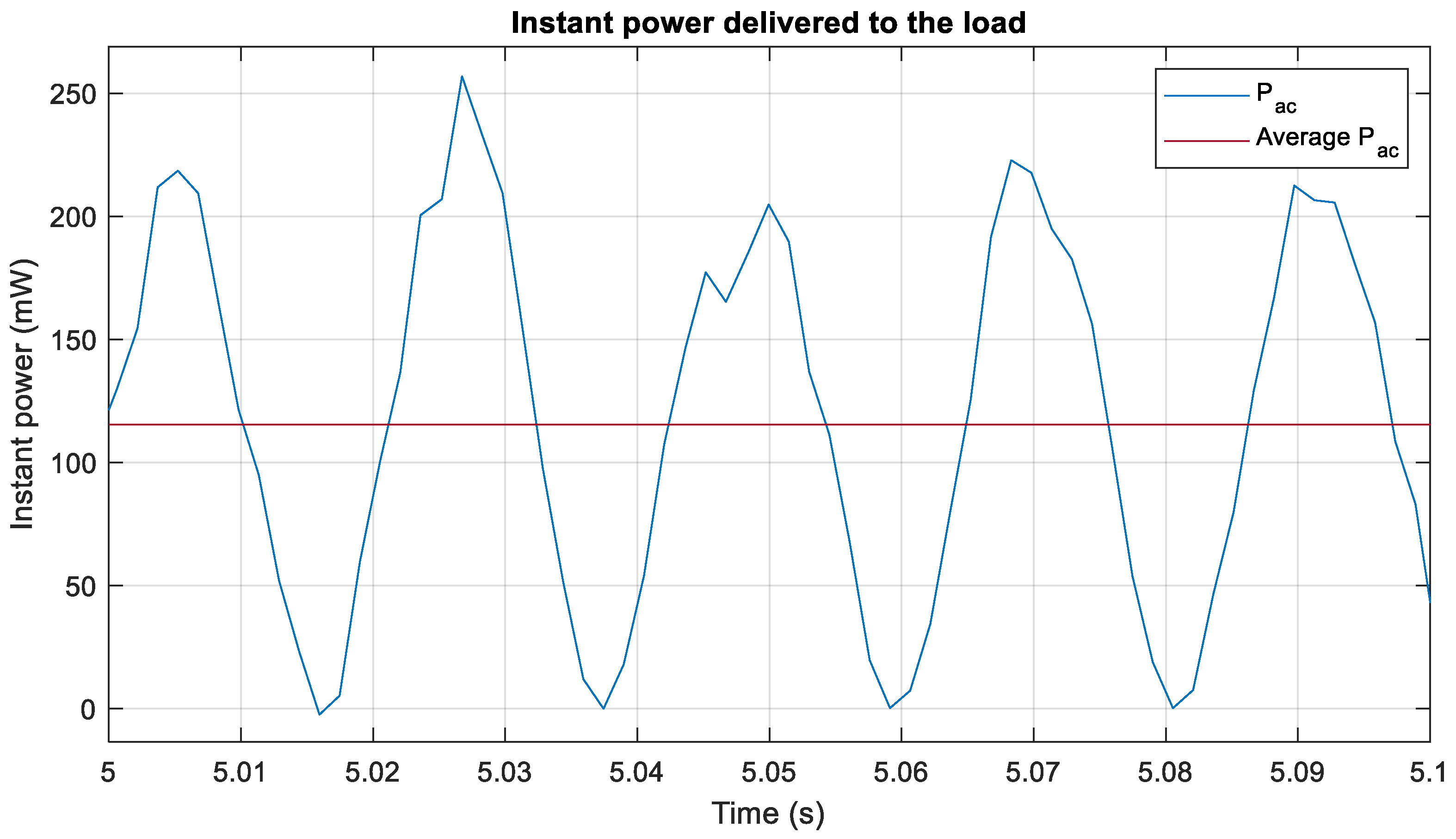
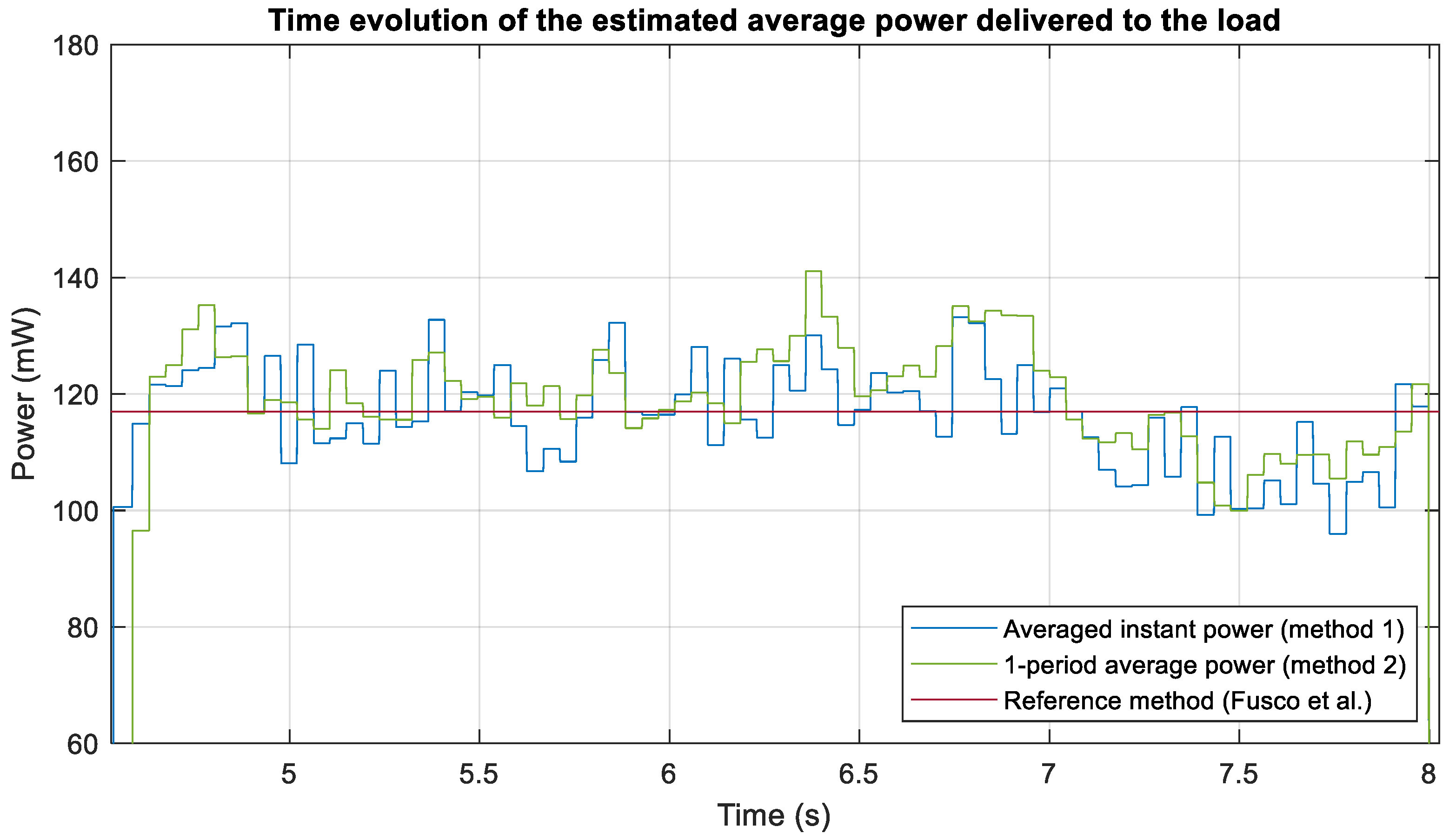
4.4. Analysis Using Experimental Measurements

In this analysis, real measurements of $P_E\left(\mathrm{t}\right)$ and $P_C\left(\mathrm{t}\right)$ were taken with the experimental setup described in [30]. As shown in Figure 17, both signals show small fluctuations, especially in their amplitude, but also in their phase and frequency. Some noise has also been observed.

Figure 17. Experimental values of $P_E\left(k\right)$ and $P_C\left(k\right)$ for measured signals, showing amplitude variations (red line).

Figure 18 shows the convergence of the DC component estimation for both $P_E\left(\mathrm{t}\right)$ and $P_C\left(\mathrm{t}\right)$. The DC component estimation algorithm shows good convergence, stabilizing after approximately three cycles, showing some small fluctuations afterwards.

Figure 18. Estimation of the DC component of the signal of $P_E\left(k\right)$ and $P_C\left(k\right)$ for measured signals.

Figure 19 compares the AC component of $P_E\left(\mathrm{t}\right)$ and $P_C\left(\mathrm{t}\right)$, both filtered and non-filtered. The moving window size for the filtering is W = 3 in all the study cases.

Figure 19. AC component of $P_E\left(k\right)$ and $P_C\left(k\right)$: non-filtered and filtered for measured signals.

Figure 20 shows the instantaneous power obtained using method 1:

Figure 20. Instantaneous power obtained using Equation (22) using measured signals.

Figure 21 shows how the estimation algorithms respond to the fluctuations observed in $P_E\left(\mathrm{t}\right)$ and $P_C\left(\mathrm{t}\right)$:

Figure 21. Evolution of the estimated average power using measured signals.

Table 7 shows the average power obtained with the proposed methods and compares them to the average power obtained with the reference procedure [17].

Table 7. Comparison of the results obtained using different methods (measured signals).

Method	Average Power (mW)	Error (%)
Reference method	116.962	--
Instantaneous power (method 1)	115.735	1.295
One-period average (method 2)	121.236	−3.654

These results show also that a good correspondence is obtained when using the three methods when using real measurements (sampled at approximately 30 measurements per period): the difference is lower than 1.3% (method 1) and 3.7% (method 2).

5. Conclusions

This paper has introduced a novel methodology for the real-time estimation of acoustic power in thermoacoustic systems, overcoming the limitations of traditional methods based on temporal averaging. The approach focuses on continuously acquiring and adjusting measurements of acoustic wave pressure, enabling the instantaneous estimation of acoustic power.

Two methods for estimating the power delivered to the load have been evaluated: (method 1) instantaneous power evaluation, which calculates the power consumed by the resistance in the RC load, and (method 2) one-period average power calculation using the well-established two-microphones method.

These methods have been validated with both different synthetic signals and experimental measurements. The results reveal that the new method provides real-time accurate estimations of the power delivered to the acoustic load and, thus, has shown potential for control-based applications.

The average power calculated by the proposed methods, compared with that obtained by the reference procedure [17], shows excellent concordance both with synthetic signals (see Table 2) and experimental measurements (Table 7).

The sensitivity analysis performed against uniformly distributed noise (see Table 3), Gaussian noise (see Table 4) and harmonic noise (see Table 5) shows that the power estimation accuracy degrades as the noise level increases. Although method 2 shows better accuracy at low noise levels, method 1 shows better robustness when the noise increases.

Another factor that has been studied is the influence of the sampling time on the average power calculated (see Table 6). The results degrade significantly when insufficient sampling (less than eight samples per cycle of the observed signals) is used. Although method 2 presents better accuracy with fine sampling, method 1 shows better robustness against coarser sampling.

This methodology allows for adaptive adjustments during operation in terms of system design and control, enhancing the overall system efficiency. Furthermore, real-time power measurement facilitates the implementation of more precise control systems, improving system performance across a range of applications.

The practical implications of this work are significant, as the methodology can be adapted for low-cost data acquisition systems, making it accessible for both commercial and research applications. The approach outlined here also offers a foundation for the development of advanced controllers in thermoacoustic engines and other similar systems, potentially paving the way for their use in sustainable energy applications.

References

- Swift, G.W. Thermoacoustics: A Unifying Perspective for Some Engines and Refrigerators, 2nd ed.; ASA Press/Springer: Cham, Switzerland, 2017; ISBN 978-3-319-66932-8. [Google Scholar]
- Backhaus, S.; Swift, G.W. A Thermoacoustic-Stirling Heat Engine: Detailed Study. J. Acoust. Soc. Am. 2000, 107, 3148–3166. [Google Scholar] [CrossRef] [PubMed]
- Farikhah, I.; Ueda, Y. Numerical Calculation of the Performance of a Thermoacoustic System with Engine and Cooler Stacks in a Looped Tube. Appl. Sci. 2017, 7, 672. [Google Scholar] [CrossRef]
- Rott, N. Damped and Thermally Driven Acoustic Oscillations in Wide and Narrow Tubes. J. Appl. Math. Phys. 1969, 20, 230–243. [Google Scholar] [CrossRef]
- Ceperley, P.H. A Pistonless Stirling Engine—The Traveling Wave Heat Engine. J. Acoust. Soc. Am. 1979, 66, 1508–1513. [Google Scholar] [CrossRef]
- Ceperley, P.H. Resonant Travelling Wave Heat Engine. U.S. Patent 4355517, 26 October 1982. [Google Scholar]
- Swift, G.W. Thermoacoustic Engines. J. Acoust. Soc. Am. 1988, 84, 1145–1180. [Google Scholar] [CrossRef]
- Ward, W.C.; Swift, G.W. Design Environment for Low-Amplitude Thermoacoustic Engines. J. Acoust. Soc. Am. 1994, 95, 3671–3672. [Google Scholar] [CrossRef]
- Zare, S.; Tavakolpour-Saleh, A.R.; Aghahosseini, A.; Mirshekari, R. Thermoacoustic Stirling Engines: A Review. Int. J. Green Energy 2023, 20, 89–111. [Google Scholar] [CrossRef]
- Iniesta, C.; Olazagoitia, J.L.; Vinolas, J.; Aranceta, J. Review of Travelling-Wave Thermoacoustic Electric-Generator Technology. Proc. Inst. Mech. Eng. Part A J. Power Energy 2018, 232, 940–957. [Google Scholar] [CrossRef]
- Chen, G.; Tang, L.; Mace, B.; Yu, Z. Multi-Physics Coupling in Thermoacoustic Devices: A Review. Renew. Sustain. Energy Rev. 2021, 146, 111170. [Google Scholar] [CrossRef]
- Backhaus, S.; Swift, G. A Thermoacoustic Stirling Heat Engine. Nature 1999, 399, 335–338. [Google Scholar] [CrossRef]
- Iniesta, C.; Olazagoitia, J.; Vinolas, J.; Gros, J. Assessing the Performance of Design Variations of a Thermoacoustic Stirling Engine Combining Laboratory Tests and Model Results. Machines 2022, 10, 958. [Google Scholar] [CrossRef]
- Nabavi, M.; Siddiqui, K. A Critical Review on Advanced Velocity Measurement Techniques in Pulsating Flows. Meas. Sci. Technol. 2010, 21, 042002. [Google Scholar] [CrossRef]
- Clapp, C.W.; Firestone, F.A. The Acoustic Wattmeter, an Instrument for Measuring Sound Energy Flow. J. Acoust. Soc. Am. 1941, 13, 124–136. [Google Scholar] [CrossRef]
- Seybert, A.F. Two-Sensor Methods for the Measurement of Sound Intensity and Acoustic Properties in Ducts. J. Acoust. Soc. Am. 1988, 83, 2233–2239. [Google Scholar] [CrossRef]
- Fusco, A.M.; Ward, W.C.; Swift, G.W. Two-Sensor Power Measurements in Lossy Ducts. J. Acoust. Soc. Am. 1992, 91, 2229–2235. [Google Scholar] [CrossRef] [PubMed]
- Luo, E.C.; Ling, H.; Dai, W.; Yu, G.Y. Experimental Study of the Influence of Different Resonators on Thermoacoustic Conversion Performance of a Thermoacoustic-Stirling Heat Engine. Ultrasonics 2006, 44, 1507–1509. [Google Scholar] [CrossRef]
- Hamood, A.; Jaworski, A.J.; Mao, X. Development and Assessment of Two-Stage Thermoacoustic Electricity Generator. Energies 2019, 12, 1790. [Google Scholar] [CrossRef]
- Backhaus, S. Initial Tests of a Thermoacoustic Space Power Engine; AIP Publishing: Melville, NY, USA, 2003; pp. 641–647. [Google Scholar]
- Tijani, M.E.H.; Spoelstra, S. A Hot Air Driven Thermoacoustic-Stirling Engine. Appl. Therm. Eng. 2013, 61, 866–870. [Google Scholar] [CrossRef]
- Yang, P.; Liu, Y.-W. Computation of the Influence of a Phase Adjuster on Thermo-Acoustic Stirling Heat Engine. J. Power Energy 2015, 229, 73–87. [Google Scholar] [CrossRef]
- Olivier, C.; Penelet, G.; Poignand, G.; Lotton, P. Active Control of Thermoacoustic Amplification in a Thermo-Acousto-Electric Engine. J. Appl. Phys. 2014, 115, 174905. [Google Scholar] [CrossRef]
- Chen, G.; Tang, L.; Yang, Z.; Tao, K.; Yu, Z. An Electret-Based Thermoacoustic-Electrostatic Power Generator. Int. J. Energy Res. 2020, 44, 2298–2305. [Google Scholar] [CrossRef]
- Iniesta, C.; Olazagoitia, J.L.; Vinolas, J.; Gros, J. New Method to Analyse and Optimise Thermoacoustic Power Generators for the Recovery of Residual Energy. Alex. Eng. J. 2020, 59, 3907–3917. [Google Scholar] [CrossRef]
- Chakradeo, A.P.; Anagolkar, S.P.; Shendge, A.B.; Pawar, P.M.; Ganeshkar, J.D. Design, Development and Manufacturing of Thermoacoustic Cooler. Int. J. Eng. Res. Technol. 2019, 8, 576–582. [Google Scholar]
- Tijani, M.E.H.; Lycklama à Nijeholt, J.A.; Spoelstra, S. Amplifying the Power Density in Thermoacoustic Systems Using a Spring Component. J. Acoust. Soc. Am. 2024, 156, 202–213. [Google Scholar] [CrossRef] [PubMed]
- Moreno, C.; González, A.; Olazagoitia, J.L.; Vinolas, J. The Acquisition Rate and Soundness of a Low-Cost Data Acquisition System (LC-DAQ) for High Frequency Applications. Sensors 2020, 20, 524. [Google Scholar] [CrossRef]
- Moreno-Ramírez, C.; Iniesta, C.; González, A.; Olazagoitia, J.L. Development and Characterization of a Low-Cost Sensors System for an Acoustic Test Bench. Sensors 2020, 20, 6663. [Google Scholar] [CrossRef]
- Iniesta, C.; Vinolas, J.; Prieto, F.; Olazagoitia, J.L.; Soliverdi, L. Experimental Performance Evaluation of a Thermoacoustic Stirling Engine with a Low-Cost Arduino-Based Acquisition System. Appl. Sci. 2024, 14, 6049. [Google Scholar] [CrossRef]
- Callanan, J.; Nouh, M. Optimal Thermoacoustic Energy Extraction via Temporal Phase Control and Traveling Wave Generation. Appl. Energy 2019, 241, 599–612. [Google Scholar] [CrossRef]
- Bertuccio, G. On the Physical Origin of the Electro-Mechano-Acoustical Analogy. J. Acoust. Soc. Am. 2022, 151, 2066–2076. [Google Scholar] [CrossRef]
- Al-Kayiem, A.; Yu, Z. Using a Side-Branched Volume to Tune the Acoustic Field in a Looped-Tube Travelling-Wave Thermoacoustic Engine with a RC Load. Energy Convers. Manag. 2017, 150, 814–821. [Google Scholar] [CrossRef]
Disclaimer/Publisher’s Note: The statements, opinions and data contained in all publications are solely those of the individual author(s) and contributor(s) and not of MDPI and/or the editor(s). MDPI and/or the editor(s) disclaim responsibility for any injury to people or property resulting from any ideas, methods, instructions or products referred to in the content. |
© 2025 by the authors. Licensee MDPI, Basel, Switzerland. This article is an open access article distributed under the terms and conditions of the Creative Commons Attribution (CC BY) license (https://creativecommons.org/licenses/by/4.0/).