Time-Efficient Path Planner in 3D Obstacle-Rich Environments Considering the Maximum Turn Rate of a Fixed-Wing Aerial Vehicle

Abstract

A time-efficient path plan algorithm is important for the real-time navigation of a fixed-wing autonomous aerial vehicle in unknown 3D obstacle-rich environments. Note that a fixed-wing aerial vehicle can freely move in 3D environments, not in 2D environments. This research addresses a 3D path planner, which is time-efficient in generating a safe and short path to the destination. In practice, a fixed-wing aerial vehicle has a limited turn rate due to its acceleration limits. The proposed path plan algorithm constructs a smooth 3D path by considering the maximum turn rate of a fixed-wing aerial vehicle. It is proven that the planned 3D path avoids collision with obstacles, while satisfying the turn rate limit constraints. Through computer simulations, one proves the outperformance (low computational load, satisfying maneuverability constraints, and short path length) of the proposed 3D path plan algorithm by comparing it with the state-of-the-art 3D rapidly exploring random tree (RRT)-based path planners considering maneuverability constraints.

1. Introduction

Currently, autonomous aerial vehicles perform various tasks, such as logistic [1,2,3], environment monitoring or target tracking tasks [4,5,6,7]. In this paper, we consider the path planning of a fixed-wing autonomous aerial vehicle. Note that a fixed-wing aerial vehicle can freely move in 3D environments, not in 2D environments. Collision-free 3D path planning is important for the safe navigation of a fixed-wing aerial vehicle in obstacle-rich uncertain 3D environments [6,8,9,10]. There can be physical obstacles, such as other aerial vehicles or buildings, as well as legal obstacles, such as areas where the drone is not allowed to fly (for example, airports, military areas, or government areas). This research therefore addresses a 3D path planner, which is time-efficient in generating a safe and short path to the destination.

In practice, a fixed-wing aerial vehicle has a limited turn rate, due to its acceleration limits [11,12,13,14,15,16,17]. Regarding 2D environments, many papers [11,12,13,15,16,17] considered a robot’s path plan while considering the robot’s acceleration limits. Regarding 2D environments, ref. [18] addressed an environment-guided variant of rapidly exploring random tree (RRT) designed for kinodynamic robot systems that incorporate a cost model to estimate the probability of collision under uncertainty in control and sensing. Regarding 2D environments, ref. [19] addressed a path-planning method for fixed-wing aerial vehicles based on the Theta-star algorithm. Ref. [19] used Euler spiral (or clothoids) to serve as connection arcs between nodes, mitigating trajectory discontinuities. Regarding 2D environments, ref. [13] addressed a fixed-wing aerial vehicle path planning algorithm for obstacle avoidance in cluttered environments. In [13], a path planning scheme was developed based on a Dubins-based improved vector field histogram for collision avoidance, satisfying the kinematic constraints of the fixed-wing aerial vehicle.

Note that a fixed-wing aerial vehicle can freely move in 3D environments, not in 2D environments. In this paper, a 3D path plan algorithm is developed by considering a limited turn rate of a fixed-wing aerial vehicle. The authors of [20] described the boundary and pointing constraints of the spacecraft trajectory planning problem based on time and path optimization. Grey wolf algorithm was used for the path planning of a spacecraft in [20]. However, the computational load of a population-based meta-heuristics algorithm, such as the grey wolf algorithm, is too heavy for real-time applications. Moreover, dynamic models of a spacecraft are different from those of a fixed-wing airplane. The authors of [21] addressed a 3D path planner, considering maneuverability constraints of an aerial vehicle. Through computer simulations, we compared the performance of the proposed path planner with [21], in order to show the outperformance of the proposed 3D path planner.

There are many research studies on 3D path plan algorithms for a robot [4]. Potential field [22], A-star algorithm [23,24,25,26], and Theta-star algorithm [27,28] can be used as 3D path plans for robots. Potential field can lead to a local minimum (not the global minimum) of the field, and thus, the robot may not reach its destination. A-star, Theta-star, or Djkstra algorithms [24,25,26,27,28] require that the entire domain consists of multiple grid cells. As one increases the domain volume, the number of grid cells required to cover the entire domain also increases. Therefore, calculating a path utilizing A-star, Theta-star, or Djkstra algorithms in a large 3D environment may not be feasible due to large computational load.

In this paper, we consider a 3D workspace domain without grid cells. Considering a domain without grid cells, the RRT algorithms in [29,30,31] applied random sampling to find a path to the destination. The authors of [30] showed that the path constructed by RRT-star converges to the optimum path asymptotically as time reaches infinity. However, we cannot wait for an infinite amount of time until we compute a solution path to the destination. The authors of [21] addressed a 3D RRT-star for computing a 3D smooth path, considering maneuverability constraints of an aerial vehicle.

In practice, a fixed-wing aerial vehicle has a limited turn rate due to its acceleration limits. In this paper, the proposed plan algorithm constructs a smooth 3D path considering the maximum turn rate of a fixed-wing aerial vehicle. It is proven that the planned 3D path avoids collision with obstacles, while satisfying the turn rate limit constraints. Through computer simulations, one proves the outperformance (low computational load, satisfying maneuverability constraints, and short path length) of the proposed path plan algorithm by comparing it with the 3D RRT-star algorithm [21], satisfying maneuverability constraints.

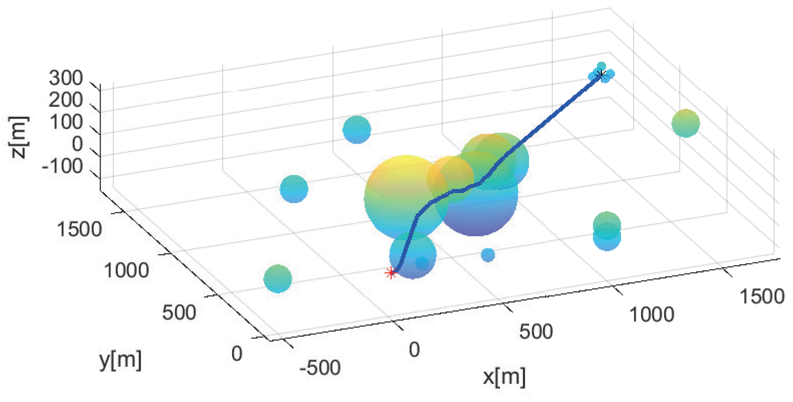
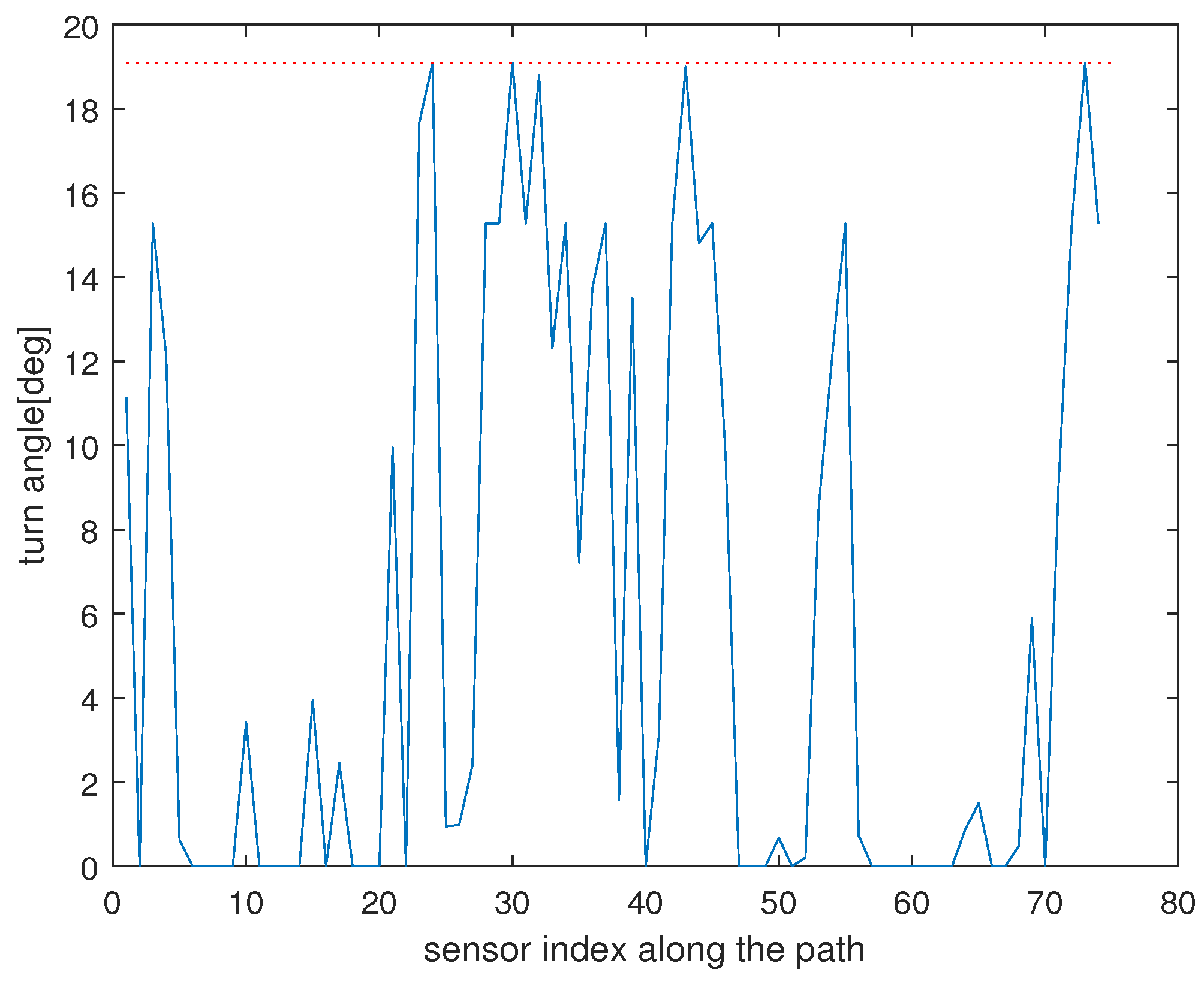
The organization of this study is as follows. Section 2 discusses assumptions and definitions. Section 3 addresses the proposed 3D path plan algorithm considering the fixed-wing aerial vehicle’s turn rate limit. Section 4 addresses the computer simulation results of the proposed path plan algorithm. Section 5 presents the conclusions.

2. Assumptions and Definitions

In this paper, a simulated vehicle and simulation nodes are used to build a 3D path while considering a limited turn rate of the aerial vehicle. Considering the fixed-wing vehicle’s limited turn rate, the simulated vehicle’s maneuver is steered to reach the destination, computing a short path to the destination. Moreover, the size of the simulated vehicle is set considering the safety margin of the constructed path.

This research applies two reference frames: a North-East-Depth (NED) reference frame $\left\{NED\right\}$ and a body-fixed reference frame $\left\{B\right\}$ [32]. The origin of $\left\{NED\right\}$ is a 3D global location with three axes pointing north, east, and depth, respectively. In addition, $\left\{B\right\}$ is fixed to the simulated vehicle’s body such that the origin of $\left\{B\right\}$ is at the vehicle’s center.

Let $\varphi$, $\theta$, and $\psi$ stand for roll, pitch and yaw, respectively. Let $c\left(\eta \right)$ stand for $\cos \left(\eta \right)$. Let $s\left(\eta \right)$ stand for $\sin \left(\eta \right)$. Let $arctan(y,x)$ stand for the angle of the complex number, for example, $x+j\ast y$.

Using [33], the matrix standing for the rotation of angle $\psi$ with respect to the z-axis in $\left\{B\right\}$ is

$$\begin{array}{c}\hfill {\mathbf{R}}_z\left(\psi \right)=\left(\begin{array}{ccc}c\left(\psi \right)& -s\left(\psi \right)& 0\\ s\left(\psi \right)& c\left(\psi \right)& 0\\ 0& 0& 1\end{array}\right).\end{array}$$

(1)

The matrix standing for the rotation of angle $\theta$ with respect to the y-axis in $\left\{B\right\}$ is

$$\begin{array}{c}\hfill {\mathbf{R}}_y\left(\theta \right)=\left(\begin{array}{ccc}c\left(\theta \right)& 0& s\left(\theta \right)\\ 0& 1& 0\\ -s\left(\theta \right)& 0& c\left(\theta \right)\end{array}\right).\end{array}$$

(2)

The matrix for the CC rotation of an angle $\varphi$ with respect to the x-axis in $\left\{B\right\}$ is

$$\begin{array}{c}\hfill {\mathbf{R}}_x\left(\varphi \right)=\left(\begin{array}{ccc}1& 0& 0\\ 0& c\left(\varphi \right)& -s\left(\varphi \right)\\ 0& s\left(\varphi \right)& c\left(\varphi \right)\end{array}\right).\end{array}$$

(3)

Using [33], the combined rotation matrix is constructed by multiplying (1), (2), and (3) as follows:

$$\begin{array}{c}\hfill \mathbf{R}(\psi ,\theta ,\varphi )={\mathbf{R}}_z\left(\psi \right){\mathbf{R}}_y\left(\theta \right){\mathbf{R}}_x\left(\varphi \right).\end{array}$$

(4)

Let destination stand for a 3D point in an open space. Let $\mathbf{D}\in {\mathcal{R}}^3$ stand for the 3D global coordinates of the destination. It is assumed that $\mathbf{D}$ is known in advance. Our goal is as follows: form a safe 3D path to the destination, so that the fixed-wing aerial vehicle with a maximum turn rate constraint can safely reach the destination in a time-efficient manner.

Consider the case where one generates a path for the aerial vehicle, whose safety margin is r. This research utilizes one simulated vehicle R to plan the path of the real aerial vehicle. Considering the safety margin r, let R stand for a sphere having radius r centered at $\mathbf{R}\in {\mathcal{R}}^3$. Here, $\mathbf{R}\in {\mathcal{R}}^3$ is the 3D global coordinates of R.

The simulated vehicle R is utilized to find a real aerial vehicle’s safe path under computer simulations. One plans the path of R with radius r, so that R avoids crossing an obstacle boundary while tracking along the path.

We acknowledge that we can regard R as a point-mass, and then add safety margin r to all obstacles. However, adding r to all obstacles can be computationally expensive, considering the case where there are many arbitrary-shaped obstacles [34]. Thus, we consider R with radius r, and collision can be checked by computing the distance between an obstacle boundary and the center of R. The safety margin r can be set, considering the vehicle’s size or the uncertainty in obstacle environments [34].

We consider a fixed-wing aerial vehicle with a constant speed, say v. We use the motion model of the aerial vehicle in [35]. Let $R_m$ denote the minimum turning radius of the vehicle in its horizontal plane. Using [35], $R_m$ is

$$\begin{array}{c}\hfill R_m={\displaystyle \frac{v^2}{g\times \tan \left(\rho \right)}}\end{array}$$

(5)

where v is the given speed of R, and $\rho$ denotes the bank angle. Also, $g=9.8$ ${\mathrm{m}/\mathrm{s}}^2$ presents the gravity acceleration constant.

Let $dt$ stand for the sampling interval in discrete-time systems. In computer simulations, one utilizes $v=20$ m/s. Then, $R_m$ = 45 m is used under [35]. Let $A_{max,z}$ denote the maximum turn angle within one sampling interval $dt$, in the vehicle’s horizontal plane. Since the simulated vehicle speed is $v>0$, $A_{max,z}$ (in radians) is given as

$$\begin{array}{c}\hfill A_{max,z}={\displaystyle \frac{v\times dt}{R_m}}.\end{array}$$

(6)

Let $A_{max,y}$ denote the maximum turn angle within one sampling interval $dt$, in the vehicle’s vertical plane. $A_{max,y}$ is given as

$$\begin{array}{c}\hfill A_{max,y}=A_{max,z}\times \rho \end{array}$$

(7)

where $\rho <1$ is a positive constant. This implies that the vehicle cannot turn a large angle in the vehicle’s vertical plane.

For computing a 3D path to the destination, R iteratively spawns simulation nodes in an open space. Let n denote an arbitrary simulation node. Let $\mathbf{n}\in {\mathcal{R}}^3$ stand for the 3D global coordinates of simulation node n.

Whenever a new simulation node is spawned, we store the node in a list, termed the simulation node list, so that all nodes in the list are sorted in the ascending order considering the relative distance to the destination $\mathbf{D}$. This implies that the first node in the list is the nearest node to $\mathbf{D}$ and that the last node in the list is the farthest node to $\mathbf{D}$.

Every simulation node n has spherical sensing coverage with a radius, say $r_s$. Here, $r_s$ is defined as

$$\begin{array}{c}\hfill r_s=v\times dt.\end{array}$$

(8)

Let $S\left(n\right)$ stand for the sphere with radius $r_s$, centered at a simulation node n. Let $\partial S\left(n\right)$ stand for the boundary of $S\left(n\right)$. Using (8), the simulated vehicle at n can reach $\partial S\left(n\right)$ within one sampling interval $dt$. An openSensingBoundary of a simulation node n stands for the set of points on $\partial S\left(n\right)$, such that every point in this set is outside an obstacle.

For the path planning of the simulated vehicle, we define the simulation graph, say G, as a tuple $G=\left(N\right(G),E(G\left)\right)$. Here, $N\left(G\right)$ is the node set, and $E\left(G\right)$ is the edge set. Each edge, e.g., $e\in E\left(G\right)$, is directed and has its weight, e.g., $w\left(e\right)>0$. Every node in $N\left(G\right)$ denotes a simulation node. Every edge, say $(n_1,n_2)\in E\left(G\right)$, implies that $\parallel {\mathbf{n}}_1-{\mathbf{n}}_2)\parallel \le \beta r_s$. Here, $\beta \ge 1$ is a constant. In computer simulations, one utilizes $\beta =1.1$. $(n_1,n_2)\in E\left(G\right)$ implies that $n_1$ and $n_2$ are one hop distance from each other. A path from $n_1$ to $n_2$ is a sequence of edges and node, such that the sequence starts from $n_1$ and ends at $n_2$.

One searches for a simulated vehicle’s path from the start to the destination. The path must be safely traversable by the simulated vehicle, which has the maximum turn angles given as (6) and (7).

Suppose that the simulated vehicle’s path from the start to the destination contains a simulation node n. Among simulation nodes along the path to reach n, $parent\left(n\right)$ is the simulation node, which is one hop distance from n. Here, $parent\left(n\right)$ is called the parent of n. Every simulation node n stores its parent as $parent\left(n\right)$. As one accesses the parent of a simulation node on the path iteratively, we can backtrack the path until meeting the start point.

Let $Line(n_1,n_2)$ stand for a straight line segment connecting two simulation nodes $n_1$ and $n_2$. $Line(n_1,n_2)$ is safe once the following safety requirement is met: while R with radius r tracks along $Line(n_1,n_2)$, R does not cross an obstacle boundary. This safety requirement can be checked by computing the distance between an obstacle boundary and $Line(n_1,n_2)$.

Suppose that the simulated vehicle has been traveling along $Line\left(parent\right(n),n)$. In the NED frame, the velocity vector of the simulated vehicle as it moves from $parent\left(n\right)$ to n is

$$\begin{array}{c}\hfill \mathbf{h}\left(n\right)={\displaystyle \frac{\mathbf{n}-\mathbf{parent}\left(n\right)}{\parallel \mathbf{n}-\mathbf{parent}\left(n\right)\parallel }}.\end{array}$$

(9)

Here, $\mathbf{n}\in {\mathcal{R}}^3$ stands for the 3D location of n, and $\mathbf{parent}\left(n\right)\in {\mathcal{R}}^3$ stands for the 3D location of $parent\left(n\right)$.

Recall that $\left\{B\right\}$ is fixed to the simulated vehicle’s body such that the origin of $\left\{B\right\}$ is at the vehicle’s center. Let $\mathbf{u}={(1,0,0)}^T$ stand for the unit velocity vector of the simulated vehicle in the body-fixed frame $\left\{B\right\}$. Utilizing (4), one applies

$$\begin{array}{c}\hfill \mathbf{h}\left(n\right)=\mathbf{R}\left(\psi \right(n),\theta (n),\varphi (n\left)\right)\times \mathbf{u}.\end{array}$$

(10)

Since $\mathbf{h}\left(n\right)$ does not consider the rolling of the vehicle, we set $\varphi \left(n\right)$ in (10) as zero. One next computes the orientation angle, e.g., $\psi \left(n\right)$ and $\theta \left(n\right)$, associated to the vehicle’s velocity vector $\mathbf{h}\left(n\right)$.

Let $\mathbf{h}(n,j)$ stand for the j-th element of $\mathbf{h}\left(n\right)$, where $j\in \{1,2,3\}$. Utilizing (10), one has

$$\begin{array}{c}\hfill \mathbf{h}\left(n\right)={(\mathbf{h}(n,1),\mathbf{h}(n,2),\mathbf{h}(n,3))}^T,\end{array}$$

(11)

Here, $\mathbf{h}(n,1)=c\left(\psi \right(n\left)\right)\times c\left(\theta \right(n\left)\right)$, $\mathbf{h}(n,2)=s\left(\psi \right(n\left)\right)\times c\left(\theta \right(n\left)\right)$, and $\mathbf{h}(n,3)=-s\left(\theta \right(n\left)\right)$. Utilizing (11), one has

$$\begin{array}{c}\hfill \theta \left(n\right)=arctan(-\mathbf{h}(n,3),\sqrt{\mathbf{h}{(n,1)}^2+\mathbf{h}{(n,2)}^2}).\end{array}$$

(12)

Utilizing (11), one computes $\psi \left(n\right)$ as follows. If $c\left(\theta \right(n\left)\right)>0$, then one utilizes

$$\begin{array}{c}\hfill \psi \left(n\right)=arctan\left(\mathbf{h}\right(n,2),\mathbf{h}(n,1\left)\right).\end{array}$$

(13)

If $c\left(\theta \right(n\left)\right)<0$, then one utilizes

$$\begin{array}{c}\hfill \psi \left(n\right)=arctan(-\mathbf{h}(n,2),-\mathbf{h}(n,1\left)\right).\end{array}$$

(14)

Recall that $\mathbf{h}\left(n\right)$ in (9) stands for the velocity vector of the simulated vehicle as it moves from $parent\left(n\right)$ to n. As the simulated vehicle starts from simulation node n, the vehicle’s turn rate is limited by its maximum turn rate. Considering the maximum turn rate $A_{max,y}$ and $A_{max,z}$ in (6) and (7), one sets feasible velocity vectors in the NED frame as

$$\begin{array}{ccc}\hfill {\mathbf{V}}_1^{NED}& =& \mathbf{R}\left(\psi \right(k),\theta (k),0)\times \mathbf{u}\hfill \\ \hfill {\mathbf{V}}_2^{NED}& =& \mathbf{R}(\psi \left(k\right),\theta \left(k\right),0)\times {\mathbf{R}}_z\left(A_{max,z}\right)\times \mathbf{u}\hfill \\ \hfill {\mathbf{V}}_3^{NED}& =& \mathbf{R}(\psi \left(k\right),\theta \left(k\right),0)\times {\mathbf{R}}_z(-A_{max,z})\times \mathbf{u}\hfill \\ \hfill {\mathbf{V}}_4^{NED}& =& \mathbf{R}(\psi \left(k\right),\theta \left(k\right),0)\times {\mathbf{R}}_y\left(A_{max,y}\right)\times \mathbf{u}\hfill \\ \hfill {\mathbf{V}}_5^{NED}& =& \mathbf{R}(\psi \left(k\right),\theta \left(k\right),0)\times {\mathbf{R}}_y(-A_{max,y})\times \mathbf{u}\hfill \\ \hfill {\mathbf{V}}_6^{NED}& =& \mathbf{R}(\psi \left(k\right),\theta \left(k\right),0)\times {\mathbf{R}}_z(A_{max,z}\times rand)\times \mathbf{u}\hfill \\ \hfill {\mathbf{V}}_7^{NED}& =& \mathbf{R}(\psi \left(k\right),\theta \left(k\right),0)\times {\mathbf{R}}_z(-A_{max,z}\times rand)\times \mathbf{u}\hfill \\ \hfill {\mathbf{V}}_8^{NED}& =& \mathbf{R}(\psi \left(k\right),\theta \left(k\right),0)\times {\mathbf{R}}_y(A_{max,y}\times rand)\times \mathbf{u}\hfill \\ \hfill {\mathbf{V}}_9^{NED}& =& \mathbf{R}(\psi \left(k\right),\theta \left(k\right),0)\times {\mathbf{R}}_y(-A_{max,y}\times rand)\times \mathbf{u}.\hfill \end{array}$$

(15)

Here, $rand$ returns a random number in the interval [0, 1].

By adding $\mathbf{n}$ to $r_s\times {\mathbf{V}}_j^{NED}$, one randomly forms the 3D global coordinates of the j-th motionPoint ($j\in \{1,2,...,q=9\}$) of n. In this way, $q=9$ random points exist on $\partial S\left(n\right)$. These $q=9$ random points are termed the viableMotionPoints of n.

Among these q viableMotionPoints, one selects a set of motionPoints, e.g., $m\left(n\right)$, satisfying the following safety requirement: the straight line segment connecting n and a point in $m\left(n\right)$ is a safe passage for the simulated vehicle R.

This safety requirement is used to avoid the case where R with radius r crosses an obstacle boundary, while R tracks along the straight line segment connecting n and a motionPoint. Suppose that the simulated vehicle R has been moving from $parent\left(n\right)$ to n. R can reach a motionPoint of n without colliding with obstacles. Thus, we say that motionPoints are reachable by R, which has been moving from $parent\left(n\right)$ to n. See Algorithm 1 for the generation of both viableMotionPoints and motionPoints. We say that a simulation node is an openSimulationNode if the simulation node has a motionPoint. We say that an openSimulationNode is closed if the node has no motionPoint.

Whenever a motionPoint is generated at a node n, we store the point in a list, termed the motionPoint list of n, so that all motionPoints in the list are sorted in ascending order, considering the relative distance to the destination $\mathbf{D}$. This implies that the first motionPoint in the list is the nearest motionPoint to $\mathbf{D}$ and that the last motionPoint in the list is the farthest motionPoint to $\mathbf{D}$.

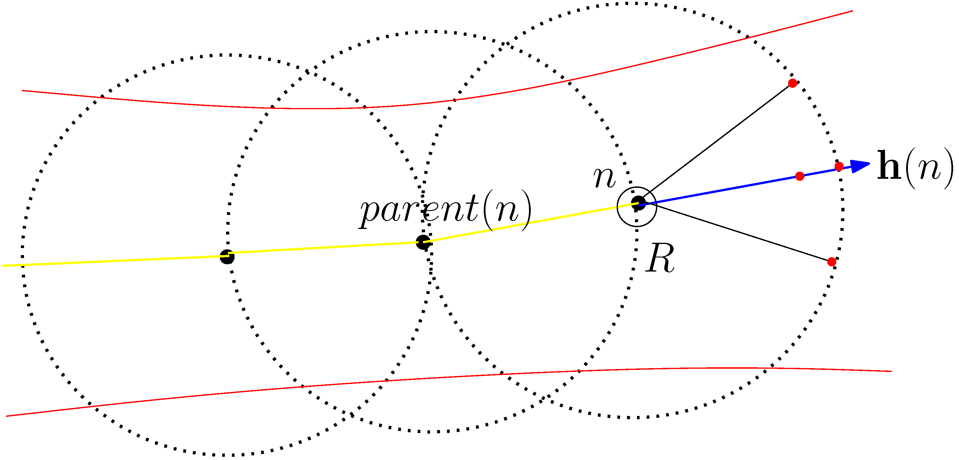
Figure 1 illustrates R spawning a new simulation node. In this figure, R is illustrated as a sphere. R maneuvers inside a tunnel, whose boundaries are illustrated as red curves. The trajectory of R is illustrated as a yellow curve. The large dots on the trajectory of R stand for the simulation nodes spawned by R. For a simulation node, say m, $\partial S\left(m\right)$ is illustrated as a dotted sphere. $\mathbf{h}\left(n\right)$ is depicted as a blue arrow emanated from n. MotionPoints are marked as large red dots on $\partial S\left(n\right)$.

Figure 1. This figure shows R spawning a new simulation node. For a simulation node, e.g., m, $\partial S\left(m\right)$ is illustrated as a dotted sphere. $\mathbf{h}\left(n\right)$ is depicted as a blue arrow emanating from n. MotionPoints are marked as large red dots on $\partial S\left(n\right)$.

3. Fast-Path-Plan Algorithm Considering the Fixed-Wing Aerial Vehicle’s Turn Rate Limit

Algorithms 1 and 2 are sub-algorithms of Algorithm 3. A time-efficient 3D path plan algorithm utilizing one simulated vehicle R is addressed in Algorithm 3.

Algorithm 3 is explained as follows. At the beginning of Algorithm 3, one forms a simulated vehicle R at the location of a real fixed-wing aerial vehicle. R spawns a simulation node at the location of a real aerial vehicle. Let $n_{init}$ stand for the first simulation node spawned at the location of the real aerial vehicle. Recall that $parent\left(n\right)$ stands for the parent of n in the simulation graph G. Initially, $\mathbf{parent}\left(n_{init}\right)$ does not exist, since $n_{init}$ is the first simulation node. Thus, we initialize $\mathbf{h}\left(n_{init}\right)$ as the heading vector of the real fixed-wing aerial vehicle in the NED frame.

Algorithm 3 iterates until the newly spawned simulation node n satisfies that R under the maximum turn rate limits ((6) and (7)) can track along the segments connecting $Line\left(parent\right(n),n)$ and $Line(n,g)$ without collisions. This implies that the simulated vehicle under the maximum turn rate limits can track along $Line(n,g)$, followed by tracking along $Line\left(parent\right(n),g)$. Thereafter, n becomes the parent of D. One then forms the shortest path from the start $n_{init}$ to the destination D by backtracking the parent relationship, starting from D. This backtracking is possible, since one reaches $n_{init}$ as one accesses the parent of a simulation node iteratively.

Algorithm 1 $GenerateOpenSimulationNode(n,parent(n)$)

1: Form q viableMotionPoints on $S_n$ using n and $parent\left(n\right)$ (see (15)); 2: for i=1:1:q do 3:    if i-th viableMotionPoint satisfies the safety requirement for a motionPoint then 4:       Store the viableMotionPoint as a motionPoint of n; 5:    end if 6: end for

Algorithm 2 R.$moveToOpenSimulationNode$

1: Among all simulation nodes, R searches for an openSimulationNode, say $n^c$, which is nearest to the destination $\mathbf{D}$; 2: $AlgorithmDone$=FALSE; 3: if no openSimulationNode can be found among all simulation nodes then 4:     $AlgorithmDone$=TRUE; 5: end if 6: Among all motionPoints of $n^c$, R finds a point which is the nearest to the destination $\mathbf{D}$, and R sets it as $f_R$; 7: R moves to $f_R$; 8: Store $n^c$ as the parent of $f_R$; 9: $f_R$ is deleted from a motionPoint of $n^c$; 10: if $n^c$ has no motionPoints then 11:     $n^c$ is closed; 12: end if

Algorithm 3 Three-dimensional path planner considering the real fixed-wing aerial vehicle’s turn rate limits

1: Let $n_{init}$ stand for the first simulation node spawned at the location of the real fixed-wing aerial vehicle; 2: Form a new simulated vehicle R at $n_{init}$; 3: repeat 4:     R spawns a new simulation node, say n, at its 3D location, if there is no simulation node at its location; 5:     $GenerateOpenSimulationNode(n,parent(n\left)\right)$ in Algorithm 1; 6:     R.$moveToOpenSimulationNode$ in Algorithm 2; 7:     if $AlgorithmDone$ is TRUE then 8:         Re-run Algorithm 3 (re-plan the path from $n_{init}$ to D); 9:     end if 10: until R under the maximum turn rate limits ((6) and (7)) can track along the segments connecting $Line\left(parent\right(n),n)$ and $Line(n,g)$ without collision; 11: Set n as $parent\left(g\right)$, the parent of the destination D; 12: Form a path from $n_{init}$ to D by backtracking the parent relationship starting from D; 13: The real fixed-wing aerial vehicle at $n_{init}$ tracks along the formed path; 14: if the real fixed-wing aerial vehicle abruptly senses a new obstacle which has not been sensed before then 15:      Delete motionPoints that are inside the newly sensed obstacle; 16:      Re-run Algorithm 3 (re-plan the path from $n_{init}$ to D); 17: end if

Recall that Algorithms 1 and 2 are sub-algorithms of Algorithm 3. Algorithm 1 is utilized to form motionPoints. Recall that a simulation node is called an openSimulationNode if the simulation node has a motionPoint. Furthermore, Algorithm 2 is utilized to make R move to an openSimulationNode, e.g., $n^c$, which is nearest to the destination $\mathbf{D}$. R moves to an openSimulationNode, which is nearest to $\mathbf{D}$, since we want to find a shortest path to $\mathbf{D}$.

Algorithm 2 is explained as follows. Under Algorithm 2, R searches for an openSimulationNode, say $n^c$, which is nearest to the destination $\mathbf{D}$. Note that an openSimulationNode can be closed as time goes on, since $f_R$ is removed from a motionPoint, as presented at the last line of Algorithm 2. R keeps searching for an openSimulationNode among all simulation nodes. If no openSimulationNode can be found, then $AlgorithmDone$ becomes true. This implies that a safe path to the destination cannot be found. Thus, we re-initialize Algorithm 3, so that the entire process for finding a safe path can be reset.

In Algorithm 2, $n^c$ is an openSimulationNode, which is nearest to the destination $\mathbf{D}$. In Algorithm 2, $f_R$ is a motionPoint of $n^c$, that will be visited by R after R moves to $n^c$. R sets a motionPoint, which is nearest to the destination, as $f_R$. Thereafter, R moves to $f_R$. Thereafter, one stores $n^c$ as a parent of $f_R$. In addition, $f_R$ is deleted from a motionPoint of $n^c$. If $n^c$ has no motionPoints, then $n^c$ is closed. Once R meets $f_R$, it spawns a new simulation node at $f_R$.

Note that R sets a motionPoint, which is nearest to the destination, as $f_R$. In this way, R is steered towards the destination. This steering movement is utilized for minimizing the path length to the destination. In short, the simulated vehicle’s maneuver is steered to reach the destination to find a short path to the destination.

Algorithm Analysis

We prove that Algorithm 3 forms a safe and smooth path, considering the maximum turn rate limits of the real aerial vehicle. Theorem 1 proves that the real aerial vehicle avoids crossing an obstacle boundary while satisfying the maximum turn rate limits, as the vehicle tracks along a path formed under Algorithm 3.

Theorem 1.

As the real fixed-wing aerial vehicle tracks along a path formed under Algorithm 3, it avoids crossing an obstacle boundary, while satisfying the maximum turn rate limits.

Proof. 

Algorithm 3 forms a path from $n_{init}$ to the destination D by backtracking the parent relationship starting from D. MotionPoints of n are reachable, as the simulated vehicle R moves from $parent\left(n\right)$ to n. Using the definition of motionPoints, a fixed-wing aerial vehicle avoids crossing obstacle boundaries as it moves from one simulation node to its motionPoint. Hence, as a vehicle moves from one simulation node towards the node’s parent, the vehicle avoids crossing obstacle boundaries.

As we generate a motionPoint, we use (15), which implies that as a vehicle moves along its generated path, the path satisfies the maximum turn rate limits. We have proven this theorem. □

We next analyze the computational complexity of Algorithm 3. Recall that whenever a new simulation node is spawned, we store the node in the simulation node list, so that all nodes in the list are sorted in the ascending order considering the relative distance to the destination $\mathbf{D}$. Also, recall that whenever a motionPoint is generated at a simulation node n, we store the point in a list, termed the motionPoint list of n, so that all motionPoints in the list are sorted in the ascending order considering the relative distance to the destination $\mathbf{D}$.

Inside the main loop of Algorithm 3, R spawns a new simulation node, e.g., n, at its 3D location, if there is no simulation node at its location. We can apply the bisection search [36] for checking if there is no simulation node at $\mathbf{n}$. Since there are $\parallel N\left(G\right)\parallel$ simulation nodes, the complexity of this search operation is $O(\parallel log(N\left(G\right))\parallel )$. Then, $GenerateOpenSimulationNode(n,parent(n\left)\right)$ is performed. The complexity of this generation operation is $O\left(q\right)$, since there are q viableMotionPoints on $S_n$.

Next, $R.moveToOpenSimulationNode$ is performed. In this algorithm, $n^c$ (a simulation node that is nearest to $\mathbf{D}$) is found among all simulation nodes. Using the simulation node list, the complexity of this search operation is $O\left(1\right)$. Then, among all motionPoints of $n^c$, R finds a point which is the nearest to the destination D, and R sets it as $f_R$. Using the motionPoint list of $n^c$, the complexity of this search operation is $O\left(1\right)$.

4. Computer Simulation Results

In this section, one proves the outperformance of our path plan algorithm (Algorithm 3) through MATLAB 2024b. simulations. Recall that [21] addressed a 3D path planner, considering maneuverability constraints of an aerial vehicle. Through computer simulations, we prove the outperformance (low computational load, satisfying maneuverability constraints, and short path length) of the proposed path planner by comparing it with the 3D RRT-star algorithm [21], satisfying maneuverability constraints.

The 3D workspace is given as $2000\times 2000\times 200$ in meters. The vehicle does not leave the workspace by regarding the workspace boundary as obstacles. We use $dt=1$ as the second sampling interval.

Considering a fixed-wing aerial vehicle, the vehicle speed is set as $v=15$ m/s. This implies that $r_s$ in (8) is 15 meters. One utilizes the safety radius of the aerial vehicle as $r=3$ m. The maximum turn angle in (6) is $A_{max,z}=19$ degrees. In (7), we use $\rho =0.8$. This implies that the vehicle cannot turn a large angle in the vehicle’s vertical plane.

The destination location is [1700, 1700, 30] in meters. The initial vehicle location is [30, 30, 30] in meters. Let L stand for the path length generated through one Monte Carlo simulation.

The authors of [30] showed that the path constructed by RRT-star converges to the optimum path asymptotically as time reaches infinity. However, one cannot wait for an infinite amount of time until the RRT-star converges. Thus, the 3D RRT-star algorithm [21] is complete as a path from the start to the destination is found.

4.1. Scenario 1

Considering Scenario 1, one presents the computer simulation results of the proposed 3D path plan algorithm (Algorithm 3). One obtains the path length as $L=2439$ in meters.

Regarding Scenario 1, Figure 2 depicts the path formed utilizing Algorithm 3. Obstacles are depicted with spheres, and the constructed smooth path is illustrated as blue line segments. The start position is marked with a red asterisk, and the destination position is marked with a black asterisk. There are several obstacles close to the destination, which makes a safe path planning more challenging. The formed path is safe for a vehicle with safety margin r meters.

Figure 2. Regarding Scenario 1, this plot shows the path formed utilizing Algorithm 3. Obstacles are depicted with spheres. The constructed smooth path is illustrated as blue line segments. The start position is marked with a red asterisk, and the destination position is marked with a black asterisk.

Regarding Scenario 1, let $[n_1,n_2,\dots ,n_{end}]$ stand for the simulation nodes along the path formed using Algorithm 3. Let $Angle\left(n_j\right)$, where $j\in \{1,2,3,\dots ,end-2\}$ stands for the angle formed by two adjacent line segments, $Line(n_j,n_{j+1})$ and $Line(n_{j+1},n_{j+2})$, in the path. Figure 3 presents $Angle\left(n_j\right)$ with respect to j, where $j\in \{1,2,3,\dots ,end-2\}$. $A_{max,z}$ is marked with a red dotted line. Note that $Angle\left(n_j\right)\le A_{max,z}$, where $j\in \{1,2,3,\dots ,end-2\}$.

Figure 3. Regarding Scenario 1, this plot shows $Angle\left(n_j\right)$ with respect to j, where $j\in \{1,2,\dots ,end-2\}$. $A_{max,z}$ is marked with a red dotted line.

Regarding Scenario 1, let $Dist\left(n_j\right)$, where $j\in \{1,2,3,\dots ,end-2\}$ stands for the relative distance between $n_j$ and its closest obstacle boundary. Figure 4 presents $Dist\left(n_j\right)$ with respect to j, where $j\in \{1,2,3,\dots ,end-2\}$. The safety radius r is marked with a red dotted line. Note that $Dist\left(n_j\right)\ge r$, where the safety radius is set as $r=3$ m.

Figure 4. Regarding Scenario 1, this plot shows $Dist\left(n_j\right)$ with respect to j, where $j\in \{1,2,\dots ,end-2\}$. The safety radius r is marked with a red dotted line.

Comparison Algorithms Through Monte Carlo Simulations

For comparison, we run the 3D RRT-star algorithm [21] considering the turn rate limits, (6) and (7). In the 3D RRT-star algorithm in [21], the steer function is used to spawn a new tree node from these two nodes: a randomly generated node and an existing tree node which is nearest to the randomly generated node. In the 3D RRT-star algorithm [21], the steer function is set considering the turn angle limits, (6) and (7). This implies that a new tree node is generated by considering the turn angle limits. In the 3D RRT-star algorithm [21], two nodes are neighbors, as their relative distance is shorter than $r_s$ in (8).

For a fair comparison, 100 Monte Carlo (MC) simulations are applied as we run the proposed plan algorithm $\left[Proposed\right]$, and the 3D RRT-star $\left[RRT\right]$. In total, 1000 tree nodes are generated in the 3D RRT-star algorithm in [21]. In the case where a safe path to the destination is not found using 1000 tree nodes, we keep re-running the associated MC simulation until a safe path to the destination is found.

In Table 1, $simTime$ (in seconds) stands for the average simulation time of running a single MC simulation utilizing MATLAB. $meanLen$ stands for the mean of path length for all MC simulations. $varLen$ stands for the variance of path length for all MC simulations. Note that the proposed plan algorithm outperforms $\left[RRT\right]$ considering both time efficiency and path length. Five hours are spent to find a path using $\left[RRT\right]$ in a single MC simulation. However, $\left[RRT\right]$ cannot succeed in finding a path within five hours. Thus, Table 1 shows - for $\left[RRT\right]$.

Table 1. Comparison analysis (Scenario 1).

$\mathit{Algorithm}$	$\mathit{simTime}$	$\mathit{meanLen}$	$\mathit{varLen}$
$\left[Proposed\right]$	163	2437	143
$\left[RRT\right]$	-	-	-

4.2. Scenario 2

Regarding Scenario 2, one presents the computer simulation results of the proposed 3D path plan algorithm (Algorithm 3). One obtains the path length as $L=2441$ in meters.

Regarding Scenario 2, Figure 5 depicts the path formed utilizing Algorithm 3. Obstacles are depicted with spheres, and the constructed smooth path is illustrated as blue line segments. The start position is marked with a red asterisk, and the destination position is marked with a black asterisk. There are several obstacles close to the destination, which makes safe path planning more challenging. The formed path is safe for a vehicle with safety margin r meters.

Figure 5. Regarding Scenario 2, this plot shows the path formed utilizing Algorithm 3. Obstacles are depicted with spheres. The constructed smooth path is illustrated as blue line segments. The start position is marked with a red asterisk, and the destination position is marked with a black asterisk.

Regarding Scenario 2, let $[n_1,n_2,\dots ,n_{end}]$ stand for the simulation nodes along the path formed using Algorithm 3. Let $Angle\left(n_j\right)$, where $j\in \{1,2,3,\dots ,end-2\}$ stands for the angle formed by two adjacent line segments, $Line(n_j,n_{j+1})$ and $Line(n_{j+1},n_{j+2})$, in the path. Figure 6 presents $Angle\left(n_j\right)$ with respect to j, where $j\in \{1,2,3,\dots ,end-2\}$. $A_{max,z}$ is marked with a red dotted line. Note that $Angle\left(n_j\right)\le A_{max,z}$, where $j\in \{1,2,3,\dots ,end-2\}$.

Figure 6. Regarding Scenario 2, this plot shows $Angle\left(n_j\right)$ with respect to j, where $j\in \{1,2,\dots ,end-2\}$. $A_{max,z}$ is marked with a red dotted line.

Regarding Scenario 2, let $Dist\left(n_j\right)$, where $j\in \{1,2,3,\dots ,end-2\}$ stands for the relative distance between $n_j$ and its closest obstacle boundary. Figure 7 presents $Dist\left(n_j\right)$ with respect to j, where $j\in \{1,2,3,\dots ,end-2\}$. The safety radius r is marked with a red dotted line. Note that $Dist\left(n_j\right)\ge r$, where the safety radius is set as $r=3$ meters.

Figure 7. Regarding Scenario 2, this plot shows $Dist\left(n_j\right)$ with respect to j, where $j\in \{1,2,\dots ,end-2\}$. The safety radius r is marked with a red dotted line.

Comparison Algorithms Through Monte Carlo Simulations

For comparison, we run the 3D RRT-star algorithm [21] considering the turn rate limits, (6) and (7). For a fair comparison, 100 Monte Carlo (MC) simulations are applied as we run the proposed plan algorithm $\left[Proposed\right]$, and the 3D RRT-star $\left[RRT\right]$. In total, 1000 tree nodes are generated in the 3D RRT-star algorithm. In the case where a safe path to the destination is not found using 1000 tree nodes, we keep re-running the associated MC simulation until a safe path to the destination is found.

In Table 2, $simTime$ (in seconds) stands for the average simulation time of running a single MC simulation utilizing MATLAB. $meanLen$ stands for the mean of path length for all MC simulations. $varLen$ stands for the variance of path length for all MC simulations. Note that the proposed 3D path plan algorithm outperforms $\left[RRT\right]$ considering both time efficiency and path length. Five hours are spent to find a path using $\left[RRT\right]$ in a single MC simulation. However, $\left[RRT\right]$ cannot succeed in finding a path within five hours. Thus, Table 2 shows-for $\left[RRT\right]$.

Table 2. Comparison analysis (Scenario 2).

$\mathit{Algorithm}$	$\mathit{simTime}$	$\mathit{meanLen}$	$\mathit{varLen}$
$\left[Proposed\right]$	164	2464	58
$\left[RRT\right]$	-	-	-

5. Conclusions

This article considers safe 3D path planning for a fixed-wing autonomous aerial vehicle. Regarding a 3D workspace domain without grid cells, this study addresses a time-efficient 3D path plan algorithm utilizing a simulated vehicle and simulation nodes. Regarding obstacle-rich 3D environments, the proposed plan algorithm generates a smooth 3D path considering the maximum turn rate of a fixed-wing aerial vehicle. This paper verifies that the proposed 3D path plan algorithm generates a short and safe path in a time-efficient manner. It is proven that the planned 3D path avoids collision with obstacles, while satisfying the turn rate limit constraints.

Through computer simulations of two cluttered environments, one proves the outperformance (low computational load, satisfying maneuverability constraints, and short path length) of our 3D path plan algorithm by comparing it with the 3D RRT-star algorithm [21] by considering the turn angle limits. As our future work, we will prove the outperformance of our 3D path plan algorithm utilizing experiments with real fixed-wing autonomous aerial vehicles. Also, in the future, we will extend the proposed 3D path planner, such that a formation of aerial vehicles can reach the destination, while considering the turn angle limit of each vehicle.