Multiscale Feature Modeling and Interpretability Analysis of the SHAP Method for Predicting the Lifespan of Landslide Dams

Abstract

Landslide dams, formed by natural disasters or human activities, pose significant challenges for lifespan prediction, which is crucial for effective water conservancy management and disaster prevention. This study proposes a hybrid CNN–Transformer model optimized using the Improved Black-Winged Kite Algorithm (IBKA) aimed at improving the accuracy of landslide dam lifespan prediction by combining local feature extraction with global dependency modeling. The model integrates CNN’s local feature extraction with Transformer’s global modeling capabilities, effectively capturing the nonlinear dynamics of key parameters affecting landslide dam lifespan. The IBKA ensures optimal parameter tuning, which enhances the model’s adaptability and generalization, especially when dealing with small-sample datasets. Experiments utilizing multi-source heterogeneous datasets compare the proposed model with traditional machine learning and deep-learning approaches, including LightGBM, MLP, SVR, CNN–Transformer, and BKA–CNN–Transformer. The results show that the IBKA–CNN–Transformer achieves R² values of 0.99 on training data and 0.98 on testing data, surpassing the baseline methods. Moreover, SHapley Additive exPlanations analysis quantifies the influence of critical features such as dam length, reservoir capacity, and upstream catchment area on lifespan prediction, improving model interpretability. This approach not only provides scientific insights for risk assessment and decision making in landslide dam management but also demonstrates the potential of deep learning and optimization algorithms in broader geological disaster management applications.

1. Introduction

Landslide dams, formed by natural disasters (e.g., earthquakes, landslides) [1,2,3] or human activities, possess unique formation mechanisms and complex internal structures. While they play crucial roles in water resource utilization, ecological protection, and disaster prevention, their stability and longevity are influenced by multiple factors [4,5], including dam material properties, environmental conditions, and hydrological variations. The failure or breach of landslide dams can trigger catastrophic floods [6], severely threatening downstream communities’ lives and property [7,8]. Therefore, accurate prediction of landslide dam longevity is vital for hydraulic engineering management, disaster prevention, and risk assessment [9,10,11].

Traditional stability analyses of landslide dams primarily rely on empirical formulas or numerical simulation methods [12], which typically conduct univariate or multivariate analyses based on geometric characteristics, material composition, or river hydrological conditions. Wu et al. [13] investigated the three-dimensional geometric evolution and influencing factors of landslide dams using Smoothed Particle Hydrodynamics (SPH), developing a predictive model for rapid dam scale calculation. Zhong et al. [14] studied dam failure mechanisms through the Tangjiashan landslide dam case and model experiments, developing a numerical model for overtopping-induced failures to precisely simulate water–soil coupling processes and breach evolution. Bout et al. [15] developed an event-based physical model for the unified simulation of earthquake-induced landslides, multi-hazard chains, and subsequent processes, achieving significant progress in multi-hazard chain simulation applicability. However, due to the heterogeneity and dynamic evolution of landslide dam formation environments, these methods show significant limitations in handling data complexity and uncertainty, often requiring extensive field monitoring data and complex modeling processes, increasing prediction costs and difficulties.

Recent advances in artificial intelligence have introduced new solutions for landslide dam longevity prediction. AI-based models demonstrate powerful modeling potential by analyzing large-scale historical data and uncovering nonlinear relationships between longevity and key parameters. Shan et al. [16] developed a novel method for rapid stability prediction using logistic regression, incorporating morphological characteristics, grain size composition, and upstream lake hydrodynamic conditions, validating its rationality through comparison with typical methods. Shi et al. [17] constructed a global landslide dam case database and utilized XGBoost models to predict stability, addressing missing data prediction challenges. Wu et al. [18] developed a Random Forest model based on geometric parameters and attribute characteristics to predict landslide dam longevity, significantly improving prediction accuracy. Liu et al. [19] studied landslide displacement prediction in the Three Gorges Dam region, comparing LSTM, Random Forest (RF), and GRU algorithms across different landslide types, with results indicating LSTM and GRU algorithms performed best in predicting step-type landslide displacements. Shi et al. [20] developed classification and regression models based on numerous landslide dam cases, providing crucial support for longevity assessment and prediction through high-precision predictions and key factor analysis. Ermini et al. [21] proposed the dimensionless blockage index as a geomorphological tool for the accurate assessment of landslide dam behavior and stability, providing a scientific basis for reducing upstream inundation risks and downstream breach flood risks. Dong et al. [22] developed a model for predicting landslide dam failure probability based on Japanese datasets, validating the model’s reliability through multiple earthquake and typhoon-induced cases, providing important references for risk assessment and disaster response. Ni et al. [23] predicted landslide displacement rates in China’s Baihetan Reservoir area using progressive deep learning and AdaBoost ensemble algorithms, demonstrating significantly improved prediction accuracy.

Although these studies have enriched the theoretical research on landslide dams, several challenges remain in longevity prediction. The diverse influencing factors of landslide dam longevity, such as geological conditions, dam materials, hydrological characteristics, and climate change, pose higher requirements for model feature extraction capabilities due to their complex interactions. Traditional deep-learning models often overfit on small datasets, limiting their adaptability to diverse scenarios. Moreover, deep-learning models are often viewed as “black boxes”, making it difficult to provide specific feature contributions and prediction rationales, limiting their practical engineering applications due to this lack of interpretability. Addressing these current research challenges, this paper proposes a hybrid IBKA–CNN–Transformer model. This model retains CNN’s advantages in local feature extraction while incorporating Transformer’s powerful global feature modeling and long-distance dependency capture capabilities, effectively addressing the modeling challenges of complex multidimensional features in landslide dam longevity prediction. Furthermore, the introduction of optimization algorithms for parameter tuning enhances the model’s adaptability and generalization capabilities under small-sample conditions. To validate model effectiveness, comprehensive experimental studies were conducted based on multi-source heterogeneous landslide dam longevity datasets, evaluating the framework’s performance in multidimensional feature input regression prediction tasks. The experimental outcomes illustrate that the model put forward remarkably surpasses the current methods in terms of prediction performance and robustness. It reveals great potential in the longevity prediction of complex systems. Additionally, this paper employs SHAP methods to interpret model outputs, quantifying feature contributions to prediction results, thereby significantly enhancing model transparency and reliability. This not only helps improve the model’s practical application value but also supports engineering managers in identifying key influencing factors and developing targeted management strategies.

This research not only provides theoretical references for innovative applications of deep-learning technology in complex system modeling but also pioneers new approaches in landslide dam longevity prediction, offering reliable tools for safety management, risk assessment, and disaster warning. The reliability of the proposed model is assessed based on its predictive performance on a separate test set. To further validate its robustness, we compared the model’s performance with baseline methods, including traditional machine-learning models (SVR, MLP, LightGBM) and deep-learning models (CNN–Transformer, BKA–CNN–Transformer). The model achieved R² values of 0.99 for the training set and 0.98 for the test set. Additionally, SHAP-based feature importance analysis was conducted to enhance the model’s interpretability, providing a deeper understanding of its decision-making process. Meanwhile, the proposed model and methods demonstrate strong generalizability, applicable to engineering problems in other complex geological environments, providing theoretical foundations and practical support for the development of intelligent prediction technologies, with significant implications for both scientific research and engineering practice.

2. Method

2.1. SVR

Support Vector Regression (SVR) fundamentally operates by finding an optimal hyperplane through support vectors within a given dataset, minimizing the deviation between predicted and actual values [24]. SVR’s strong generalization capability makes it suitable for handling high-dimensional data and nonlinear regression problems.

SVR employs an $\delta$-insensitive loss function to constrain error ranges, ensuring small errors do not impact model optimization. The following is the specific definition:

$$L(z,g(x))=\left\{\begin{array}{cc}0& \mathrm{if} \left|z-g(x)\le \delta \right|\\ \left|z-g(x)\right|& \mathrm{if} \left|z-g(x)>\delta \right|\end{array}\right.$$

(1)

where $\delta$ represents the allowable error range.

The optimization objective of SVR is to minimize both model complexity and total loss exceeding the error range:

$$\underset{v,c,\eta ,{\eta }^{\ast }}{\min }{\displaystyle \frac{1}{2}}{‖v‖}^2+D{\displaystyle \sum _{j=1}^m({\eta }_j+}{\eta }_j^{\ast })$$

(2)

where $v$ is the model weight vector; ${\eta }_j$ and ${\eta }_j^{\ast }$ are slack variables representing errors exceeding $\delta$; and $D$ is the regularization parameter controlling the trade-off between model complexity and error.

It is subject to the following constraints:

$$\left\{\begin{array}{c}{z}_j-(v^T\psi (x_j)+c)\le \delta +{\eta }_j\\ (v^T\psi (x_j)+c)-z_j\le \delta +{\eta }_j^{\ast }\\ {\eta }_j,{\eta }_j^{\ast }\ge 0\end{array}\right.$$

(3)

Through the kernel function $Q(x_i,x_k)=\psi {(x_i)}^T\psi (x_k)$, the optimization problem can be transformed into its dual form,

$$\underset{\beta ,{\beta }^{\ast }}{\max }(-{\displaystyle \frac{1}{2}}{\displaystyle \sum _{i,k=1}^m({\beta }_i-}{\beta }_i^{\ast })Q(x_i,x_k)+{\displaystyle \sum _{i=1}^m({\beta }_i-}{\beta }_i^{\ast })z_i-\delta {\displaystyle \sum _{i=1}^m(}{\beta }_i+{\beta }_i^{\ast }))$$

(4)

subject to the following constraints:

$$\left\{\begin{array}{c}{\displaystyle \sum _{i=1}^m({\beta }_i-}{\beta }_i^{\ast })=0\\ 0\le {\beta }_i,{\beta }_i^{\ast }\le D\end{array}\right.$$

(5)

The final regression prediction function is as follows, where the key parameters are determined by the optimization process:

$$g(x)={\displaystyle \sum _{i=1}^m({\beta }_i-{\beta }_i^{\ast })Q(x_i,x)+c}$$

(6)

where ${\beta }_i$ and ${\beta }_i^{\ast }$ are Lagrange multipliers obtained by optimization.

2.2. LightGBM

Light Gradient Boosting Machine (LightGBM) is an improved Gradient Boosting Decision Tree (GBDT) framework characterized by high training efficiency, low memory footprint, and excellent prediction accuracy [25]. The framework dramatically improves the training efficiency and resource utilization of the model through innovative techniques such as leaf-wise splitting strategy (leaf-wise), histogram optimization, gradient one-sided sampling (GOSS), and mutually exclusive feature bundling (EFB).

LightGBM significantly reduces computational complexity by fitting residuals to approximate the objective function at each iteration, and it adopts feature discretization and sample optimization strategies to build efficient and powerful integrated models. During the model construction process, LightGBM is based on a decision tree that integrates multiple weak learners into one strong learner to improve the overall prediction performance. Here is the core formula:

$$Z_n(x)=Z_{n-1}(x)+\eta ·h_n(x)$$

(7)

where $Z_n(x)$ denotes the predicted value of the $n$th round, $\eta$ is the learning rate, and $h_n(x)$ is the weak learner of the current round.

2.3. MLP

The Multi-Layer Perceptron, commonly abbreviated as MLP, falls into the type of feed-forward neural networks, which is one of the most basic models in deep learning [26]. The model mainly consists of input, hidden, and output layers.

Through forward propagation, the MLP calculates the activation values of the hidden layer, layer by layer:

$$a^{(n)}=\sigma (W^{(n)}{a}^{(n-1)}+b^{(n)})$$

(8)

where $\sigma$ is the activation function and $W^{(n)}$ and $b^{(n)}$ denote the weight matrix and bias vector, respectively.

To optimize the model, the MLP employs the mean square error (MSE) loss function to assess the error between the predicted and true values, and it updates the weights and biases by calculating the gradient through a back-propagation algorithm. The update formula is as follows:

$$W^{(n)}=W^{(n)}-\eta ·{\displaystyle \frac{\partial L}{\partial W^{(n)}}}$$

(9)

where $\eta$ is the learning rate.

2.4. Transformer

The Transformer model is an advanced deep-learning framework that utilizes the self-attention mechanism, originally developed for sequence-to-sequence tasks. However, its sophisticated properties render it highly suitable for a broad spectrum of applications. The model is composed of two primary components: an encoder and a decoder [27,28]. The principle of the model is as follows:

2.4.1. Embedding Position and Position Encoding

Since the Transformer does not have recursive properties, it is necessary to introduce information about the order of each element in the input sequence through position encoding. For the input vector $X$, it is passed through the embedding layer to obtain the vector $E(X)$, and then superimposed with the position encoding $PE$ to obtain the final input vector:

$$Z_o=E(X)+PE$$

(10)

The position encoding uses sine and cosine functions, as in the following equation:

$$PE(pos,2i)=\sin ({\displaystyle \frac{pos}{{1000}^{2i/d_{model}}}})$$

(11)

$$PE(pos,2i+1)=\cos ({\displaystyle \frac{pos}{{1000}^{2i/d_{model}}}})$$

(12)

where $pos$ is the position index, $i$ is the dimension index, and $d_{model}$ is the dimension of the embedding vector.

2.4.2. Multi-Head Attention Mechanism

The multi-head self-attention mechanism is at the heart of Transformer and is used to capture relationships between input vectors. For the input matrix $Z\in R^{n\times d_{model}}$ (containing $n$ input vectors), the attention value is calculated as follows.

$$Q=Z{W}^Q$$

(13)

$$K=Z{W}^K$$

(14)

$$V=Z{W}^V$$

(15)

$$Attention(Q,K,V)=\mathrm{softmax}({\displaystyle \frac{Q{K}^T}{\sqrt{d_k}}})V$$

(16)

$$\mathrm{MultHead}(Q,K,V)=\mathrm{Concat}(hea{d}_1,\dots ,hea{d}_h)W^O$$

(17)

where $W^Q,W^K,W^V\in R^{d_{model}\times d_k}$ is the learnable weight matrix; $Q,K,V$ are the query, key and value matrices, respectively; $Q{K}^T$ computes the click similarity between the query and the key; $\sqrt{d_k}$ is the scaling factor to avoid large values that cause the gradient to vanish; $\mathrm{softmax}$ is used to normalize the weights; and $hea{d}_i=Attention(Q{W}_i^Q,K{W}_i^K,V{W}_i^V)$, $W^O\in R^{h{d}_k\times d_{model}}$ are the projection matrices.

2.4.3. Forward Fully Connected Networks

Each attention layer is followed by a forward fully connected network for further processing of features. This network contains two linearly transformed live functions:

$$\mathrm{FEN}(x)=\mathrm{ReLU}(x{W}_1+b_1)W_2+b_2$$

(18)

where $W_1$, $W_2$, $b_1$, and $b_2$ are learnable parameters.

2.4.4. Overall Model Output

After $L$ layers of stacked encoders, the final hidden representation $z_L$ is obtained, and then the hidden representation is mapped to the predicted values through linear layers:

$$\widehat{y}=z_L{W}_y+b_y$$

(19)

where $W_y\in R^{d_{model\times 1}}$ and $b_y$ is the bias term.

2.4.5. Loss Function

For the regression prediction task, the root-mean-square error (RMSE) is used as the loss function,

$$L={\displaystyle \frac{1}{N}}{\displaystyle \sum _{i=1}^N{({\widehat{y}}_i-y_i)}^2}$$

(20)

where $N$ is the number of samples, ${\widehat{y}}_i$ is the predicted value, and $y_i$ is the true value.

2.5. CNN–Transformer

The convolutional neural network (CNN) is a model with high feature extraction capability [29,30] that extracts local features of the input data through convolutional layers, reduces the model complexity by using weight sharing and local connectivity, and reduces the dimensionality through pooling layers to retain key information and reduce noise. The feature extraction capability of the convolutional layer enables it to capture local correlations between input variables, the activation function introduces nonlinear mapping to enhance the model’s representation, and finally, the extracted high-dimensional features are mapped to the regression output through the full connectivity layer to achieve accurate prediction of the target variables. The model shows high efficiency and good generalization ability when dealing with multidimensional features or data with spatial distributions.

The CNN–Transformer model [31] realizes efficient modeling and prediction of complex data patterns in regression prediction. It does this by integrating the local feature extraction ability of CNN with the global modeling ability of Transformer. The CNN module first extracts local features from the input data, and then extracts the local correlation or feature interaction information and uses it for regression prediction. The Transformer module [32] uses the self-attention mechanism to capture the global dependencies among the features, thus modeling the potentially complex nonlinear relationships in the data. Ultimately, the Transformer output goes through a linear layer to complete the regression prediction. The model can efficiently process local information and fully model global features, which is suitable for regression tasks on structured or unstructured data with excellent prediction accuracy and generalization ability. The schematic diagram of the CNN–Transformer model is shown in Figure 1.

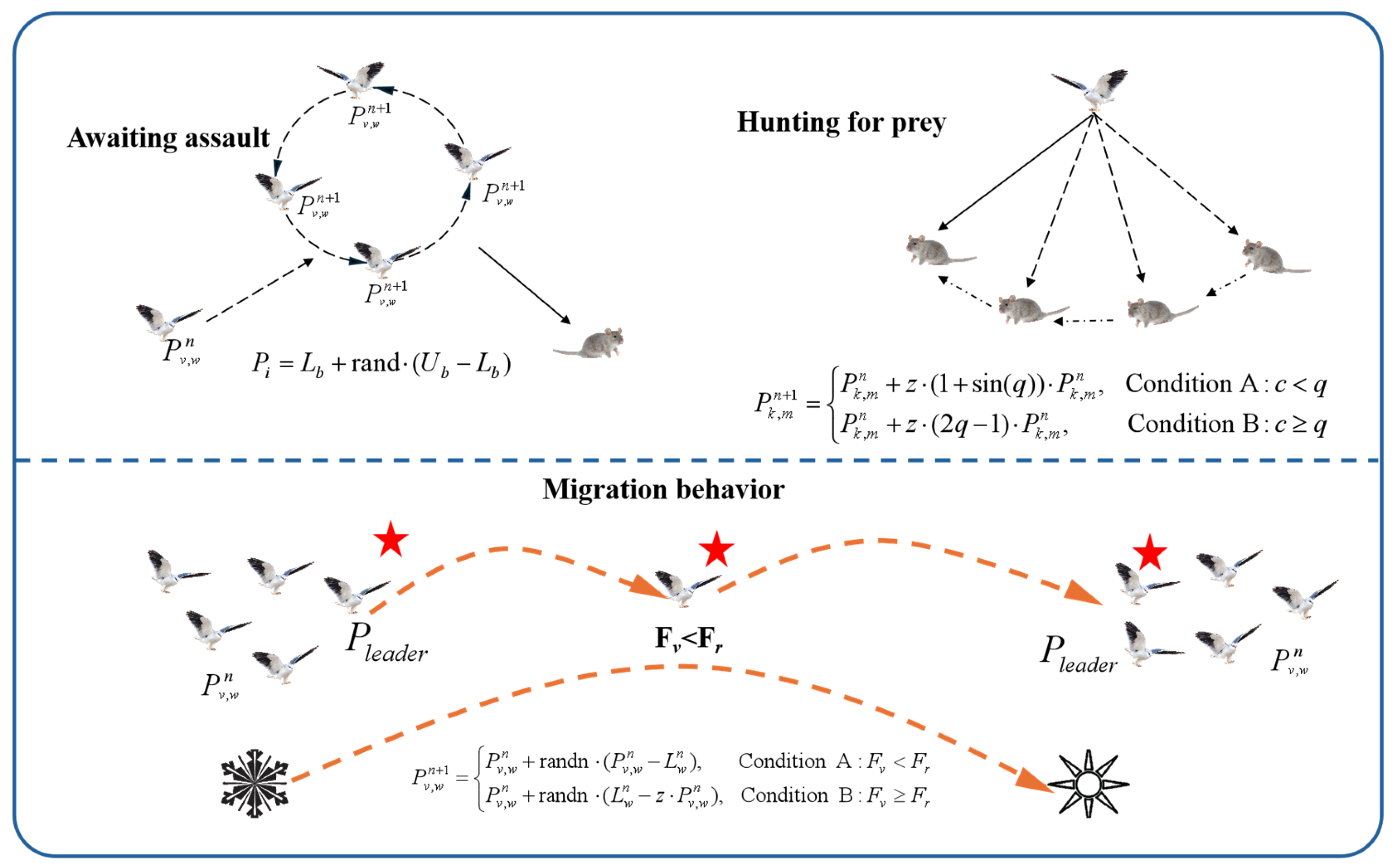
2.6. Black-Winged Kite Algorithm

The Black-Winged Kite Algorithm (BKA) is a novel meta-heuristic optimization algorithm [33] that simulates the hunting and migratory behaviors of the black-winged kite in order to solve complex optimization problems. Figure 2 depicts the schematic diagram of the algorithm.

2.6.1. Stochastic Initialization of Population Positions

Generate random individual positions in the initial solution space,

$$P_i=L_b+\mathrm{rand}·(U_b-L_b)$$

(21)

where $L_b$ and $U_b$ are the lower and upper bounds of the search range, respectively, and rand is a random number within [0,1].

2.6.2. Hunting Behavior

The trapping behavior implements global and local search through sinusoidal and exponential functions to quickly locate potentially optimal regions:

$$P_{k,m}^{n+1}=\left\{\begin{array}{ll}{P}_{k,m}^n+z·(1+\sin (q))·P_{k,m}^n,& \mathrm{Condition} \mathrm{A}:c<q\\ P_{k,m}^n+z·(2q-1)·P_{k,m}^n,& \mathrm{Condition} \mathrm{B}:c\ge q\end{array}\right.$$

(22)

$$z=0.05·e^{-2·{(n/N)}^2}$$

(23)

where $n$ corresponds to the current iteration number and $N$ corresponds to the total iteration number; $q$ is a random number within [0,1]; $c=0.9$.

2.6.3. Migration Behavior

When the current environment is poor or food is scarce, the algorithm simulates the migratory behavior of the black-winged kite population and jumps out of the local optimal solution by selecting a new leader:

$$P_{v,w}^{n+1}=\left\{\begin{array}{ll}{P}_{v,w}^n+\mathrm{randn}·(P_{v,w}^n-L_w^n),& \mathrm{Condition} \mathrm{A}:F_v<F_r\\ P_{v,w}^n+\mathrm{randn}·(L_w^n-z·P_{v,w}^n),& \mathrm{Condition} \mathrm{B}:F_v\ge F_r\end{array}\right.$$

(24)

$$z=2·\sin (q+\pi /2)$$

(25)

where $F_v$ is the fitness value of the current individual, $F_r$ is the fitness value of the random individual, and $L_w^n$ is the position of the current leader.

2.6.4. Optimal Value Selection

The individual with the current optimal adaptation is selected as the leader:

$$f_{\min }=\min (f(P_i))$$

(26)

$$P_{\mathrm{leader}}=P(find(f_{\min }==f(P_i)))$$

(27)

2.7. Improved Black-Winged Kite Algorithm (IBKA)

Considering that the BKA algorithm lacks dynamic adaptation, it tends to lose the diversity of the population, and the parameters present in it are relatively fixed and lack the ability of hierarchical search. Therefore, the study proposes an IBKA algorithm, which can dramatically improve the algorithm’s global search ability, local optimization ability, and stability of the results through the dynamic adaptive mechanism, the population clustering strategy, and the dynamic migration strategy.

In comparison with traditional optimization algorithms such as the Genetic Algorithm (GA) and Particle Swarm Optimization (PSO), the IBKA offers several notable advantages. On the one hand, GA operates based on evolutionary principles, using crossover and mutation operations, which can result in a slower convergence rate and a higher chance of becoming stuck in local optima due to its reliance on predefined genetic operators. PSO, on the other hand, relies on a swarm of particles exploring the search space, but this method can suffer from premature convergence if the swarm lacks diversity, especially in complex, high-dimensional problems. In contrast, IBKA incorporates dynamic adaptation mechanisms that allow it to adjust its search process over time, enhancing its ability to explore the search space more thoroughly. The introduction of population clustering and dynamic migration strategies in IBKA further improves its robustness and avoids the pitfalls of local optima. These enhancements lead to faster convergence, higher-quality solutions, and better adaptability in complex, high-dimensional optimization problems, such as those encountered in our study. The IBKA’s superior ability to maintain diversity within the population and adaptively fine-tune the optimization process provides a clear advantage over GA and PSO in the context of solving intricate optimization problems like the one discussed in this research.

2.7.1. Initializing the Population

Similar to the original BKA, the population initialization equation is

$$P_i=L_b+\mathrm{rand}·(U_b-L_b)$$

(28)

where $L_b$ and $U_b$ are the lower and upper bounds of the search range, respectively; $\mathrm{rand}$ is a random number within [0,1].

2.7.2. Adaptive Trapping Behavior

A dynamic learning rate $\eta$ is introduced to dynamically adjust the trapping step size according to the number of iterations:

$$\eta ={\eta }_{\max }·(1-{\displaystyle \frac{n}{N}})+{\eta }_{\min }·{\displaystyle \frac{n}{N}}$$

(29)

The trapping behavior equation is

$$P_{k,m}^{n+1}=\left\{\begin{array}{ll}{P}_{k,m}^n+\eta ·(1+\sin (q))·P_{k,m}^n,& \mathrm{Condition} \mathrm{A}:c<q\\ P_{k,m}^n+\eta ·(2q-1)·P_{k,m}^n,& \mathrm{Condition} \mathrm{B}:c\ge q\end{array}\right.$$

(30)

where ${\eta }_{\max }$ and ${\eta }_{\min }$ are the initial and minimum values of the learning rate, $n$ is the current number of iterations, and $N$ is the maximum number of iterations; the rest of the symbols have the same meaning as in the original BKA.

2.7.3. Population Clustering Strategy

The population is divided into $G$ clusters, and individuals within each cluster use independent hunting strategies. The cluster division formula is as follows:

$$G_j=\left\{P_i\left|\right.\right. \left.‖P_i-P_{\mathrm{leader}}‖<{\tau }_j\right\}$$

(31)

where ${\tau }_j$ is the radius of the cluster; the center of the cluster is the current leader $P_{\mathrm{leader}}$.

Individuals in each cluster interact with the following information after hunting:

$$P_{j,i}^{n+1}=\lambda ·P_{j,i}^n+(1-\lambda )·P_{\mathrm{leader}}^n$$

(32)

where $\lambda$ is the fusion coefficient, which usually takes values in the range of $[0.5,0.9]$.

2.7.4. Dynamic Migration Strategies

Dynamically adjust the migration probability based on individual adaptation:

$$P_{\mathrm{migrate}}={\displaystyle \frac{F_{\max }-F_i}{F_{\max }-F_{\min }+\epsilon }}$$

(33)

The migratory behavior equation is

$$P_{v,w}^{n+1}=\left\{\begin{array}{ll}{P}_{v,w}^n+\mathrm{randn}·(P_{v,w}^n-L_w^n),& \mathrm{Condition} \mathrm{A}:\mathrm{rand}<P_{\mathrm{migrate}}\\ P_{v,w}^n+\mathrm{randn}·(L_w^n-z·P_{v,w}^n),& \mathrm{Condition} \mathrm{B}:\mathrm{rand}\ge P_{\mathrm{migrate}}\end{array}\right.$$

(34)

where $F_{\max }$ and $F_{\min }$ are the maximum and minimum fitness of the population, respectively; $\epsilon$ is a constant that prevents the denominator from being zero.

2.7.5. Optimal Value Selection

As in the original BKA, select the current optimal individual:

$$f_{\min }=\min (f(P_i))$$

(35)

$$P_{\mathrm{leader}}=P(find(f_{\min }==f(P_i)))$$

(36)

2.8. CNN–Transformer Hybrid Model Based on IBKA

In order to achieve accurate predictions of weir dam life, a CNN–Transformer hybrid model based on the Improved Black-Winged Kite Optimization Algorithm (IBKA) is suggested in this study. The method combines the quantitative features of weir dams (e.g., dam height, dam width, and dam volume) and qualitative features (e.g., triggering factors and material types) to fully utilize the complementary advantages of the two types of features. The model uses CNN to extract local patterns from quantitative features and discovers intrinsic geometric patterns through convolution and pooling operations; subsequently, the Transformer module further captures the global feature interactions through the multi-head self-attention mechanism, especially the combined effects of triggering factors and material types on the lifespan.

The Improved Black-Winged Kite Algorithm (IBKA) is utilized to optimize key hyperparameters in the CNN–Transformer hybrid model, ensuring enhanced convergence efficiency and predictive performance. Specifically, IBKA fine-tunes the convolutional kernel size in the CNN component, which significantly impacts the model’s ability to extract local features. A larger kernel captures broader patterns, whereas a smaller kernel enables fine-grained feature extraction, and IBKA dynamically balances this trade-off to improve feature representation while maintaining computational efficiency. Additionally, IBKA optimizes the number of Transformer layers, a critical factor in capturing long-range dependencies and complex global interactions. While increasing the number of layers enhances the model’s capacity for learning intricate relationships, excessive layers may lead to overfitting or prolonged training time; thus, IBKA ensures an optimal depth that maximizes learning efficiency without compromising generalization. Furthermore, IBKA fine-tunes the number of attention heads, which determines the degree of parallelization in the Transformer’s multi-head attention mechanism. More attention heads enable the model to capture diverse feature relationships, particularly in high-dimensional data, but an excessive number may increase computational cost and reduce training efficiency. By systematically optimizing these hyperparameters, IBKA accelerates model convergence, improves predictive accuracy, and enhances the generalization capability of the CNN–Transformer hybrid model, allowing it to effectively capture both local and global dependencies in landslide dam lifespan prediction.

Finally, the optimized model is used for training, based on the mean square error (MSE) as the objective function, and the prediction accuracy is evaluated using the test set. The method provides an efficient and reliable solution for weir life prediction by combining the local and global feature modeling capabilities, and at the same time, demonstrates strong practicality and robustness in handling mixed feature data. The framework diagram of the intelligent prediction model used to predict weir life is shown in Figure 3.

2.9. Managing Uncertainty in Input Parameters: A Probabilistic Approach

To enhance the ability of the IBKA–CNN–Transformer model to handle uncertainties in input parameters, this study introduces a probabilistic approach designed to capture the variability of key input parameters. Landslide dam lifespan prediction is influenced by numerous uncertain factors, including hydrological conditions, dam geometry, and material properties, which can fluctuate due to environmental changes, measurement errors, and natural variability. As such, properly accounting for these uncertainties in the model is crucial for improving prediction reliability and generalization.

To model these uncertainties, appropriate probability distributions are assigned to each key input parameter, such as rainfall intensity, upstream catchment area, dam height, dam width, and material strength. These distributions are selected based on historical data analysis and expert domain knowledge. By adopting this approach, the model avoids treating parameters as fixed values, allowing them to vary within a defined range, thereby providing a more accurate representation of the uncertainty inherent in real-world scenarios. The Monte Carlo simulation method [34] is employed to implement this probabilistic approach. Each input parameter is sampled randomly, and the model is iteratively run to generate multiple lifespan predictions. This process produces uncertainty intervals for each prediction, thus overcoming the limitations of traditional methods, which typically provide only a single deterministic forecast. By adopting this approach, we obtain a distribution of predictions, each associated with a confidence level, and can further assess the risks involved.

Ultimately, this probabilistic modeling approach enables a more comprehensive risk assessment. It not only quantifies the uncertainty in the predictions but also assists decision makers in evaluating potential risks. This methodology significantly improves the model’s applicability and reliability in practical engineering contexts, particularly for managing uncertainties in complex systems like landslide dam lifespan prediction.

3. Database

3.1. Data Sources

The data for this study were obtained from the research of Fan [35] and Shen [36], both focusing on landslide dams formed by natural mass movements such as landslides, rockslides, or debris avalanches. These dams, resulting from various types of mass movements, exhibit different material compositions, including rock, debris, and soil. These dams were not human-made but are the result of natural processes. Fan [35] compiled a global database of 410 landslide dams, each with a volume greater than 1 million m³, formed since 1900. This database includes detailed information on dam longevity and stability along with key parameters such as landslide type, dam material, and geomorphological features known to influence dam lifespan. The dataset plays a vital role in identifying trends, particularly the relationship between dam material and longevity. Shen [36], in contrast, focused on the full longevity of landslide dams, which was divided into three stages: infilling, overflowing, and breaching. The study developed regression models to estimate the total longevity, incorporating dam characteristics, hydrological conditions, and triggering factors (e.g., rainfall and earthquakes). The dataset used by Shen [36] is enriched with multi-dimensional data on triggering factors, dam materials, and geometric/hydrological parameters, all essential for estimating dam lifespan across the different stages. These comprehensive datasets from both sources provide a solid foundation for modeling dam longevity under varying environmental conditions and offer robust data for assessing dam stability and failure risk.

To ensure the inclusion of the most critical features for landslide dam lifespan prediction, the study refers to the method of Shi [20] et al. for scientific selection and the optimization of key indicators; furthermore, a structured feature selection process is employed, integrating correlation analysis, domain expertise, and SHAP analysis. Initially, Pearson correlation analysis was conducted to evaluate the relationships between features and to identify highly correlated or redundant variables, ensuring that selected features contribute uniquely to the model. The detailed results of the correlation analysis are provided in Section 3.4. Expert knowledge from the field of geotechnical and hydrological engineering was also incorporated to retain critical variables that are known to impact dam stability; these indicators cover multiple dimensions such as dam size, upstream catchment area, triggering factors, and dam materials of weir dams, which systematically characterize the core factors affecting the stability and lifetime of weir dams. Following model training, SHAP analysis was subsequently used to quantify the contribution of each selected feature to the model’s predictions, offering further insights into the importance of these features and validating the feature selection process. This systematic approach ensures that the final feature set maintains both predictive efficiency and practical significance, enhancing model generalization and interpretability.

The dam scale includes dam height, dam length, dam width, dam volume, and weir volume, which directly determine the performance of a weir dam in terms of external pressure and internal stability; among these, the dam height affects the sliding resistance of the dam body, the dam length and dam width reflect the planar scale of the dam body and the contact area of the substrate, the dam volume reveals its ability to withstand gravity and seismic effects, and the weir volume is directly related to the water pressure changes and their potential threat to the dam body. The upstream catchment area, as a determinant of the regional hydrological catchment, directly affects the weir’s water reserve and dam water pressure. The larger its value, the higher the hydrodynamic load triggered by rainfall or snowmelt in the watershed, thus increasing the risk of dam instability. In terms of triggering factors, earthquakes, rainfall/snowmelt, and other external events are the main triggers for sudden weir destabilization, and the intensity and frequency of different triggering mechanisms significantly affect their lifetimes. Earthquakes can weaken the structural stability of dams through strong surface movements, rainfall and snowmelt increase water pressure and reduce the material friction coefficients, and other factors, such as volcanic eruptions or landslides, may trigger transient damage. In addition, the dam material is an important variable in determining its physical stability and damage resistance. Rock, debris, and earth materials have different impacts on the life distribution of dams due to the differences in mechanical properties; rock dams are relatively stable but sensitive to cracks, debris dams are more sensitive to erosion, and earth dams are easily destabilized by rainfall or seepage.

3.2. Data Preprocessing

In this study, the data collected from previous research on landslide dams included several variables such as dam scale, upstream catchment area, triggering factors, and dam materials (Some initial data are provided in the Supplementary Materials). To ensure the validity and reliability of the data, two critical preprocessing steps were applied: elimination of outliers and interpolation of missing data. The procedure for eliminating outliers was performed by using statistical methods such as Z-scores and IQR (Interquartile Range). Any data points that were beyond the thresholds defined by these methods were considered outliers and removed from the dataset.

For the missing data, interpolation methods were carefully selected based on the nature and distribution of the variables. For continuous variables, linear interpolation was used when there was a small proportion of missing values. In cases where larger amounts of missing data were present, more sophisticated techniques such as multiple imputation were employed. These steps ensure that the dataset is complete and robust for subsequent modeling. After these procedures, the final dataset comprised 297 valid records, with 80% used for training and 20% for testing.

3.3. Data Description and Analysis

Table 1. Statistical characteristics of the datasets.

Parameter	STD	Kurt	Max	Min	Mean	Median	Range
Dam height (m)	84.32	52.90	1000	2	61.76	32	998
Dam length (m)	425.13	24.36	4000	5	367.50	250	3995
Dam width (m)	729.50	13.73	6000	20	612.44	350	5980
Dam volume (106 m3)	216.24	125.91	3000	0.01	36.84	1.90	2999.99
Dammed lake volume (106 m3)	187.16	19.89	1500	0	71.85	4.10	1500
Upstream catchment area (km2)	21,993.36	45.62	173,484	0.60	4298.30	98.70	173,483.40
Triggers (earthquake)	0.50	−1.92	1	0	0.43	0	1
Triggers (rainfall and snowmelt)	0.50	−1.99	1	0	0.48	0	1
Triggers (others)	0.28	6.52	1	0	0.09	0	1
Dam material (rock)	0.48	−1.62	1	0	0.35	0	1
Dam material (debris)	0.49	−1.84	1	0	0.40	0	1
Dam material (earth)	0.43	−0.61	1	0	0.25	0	1
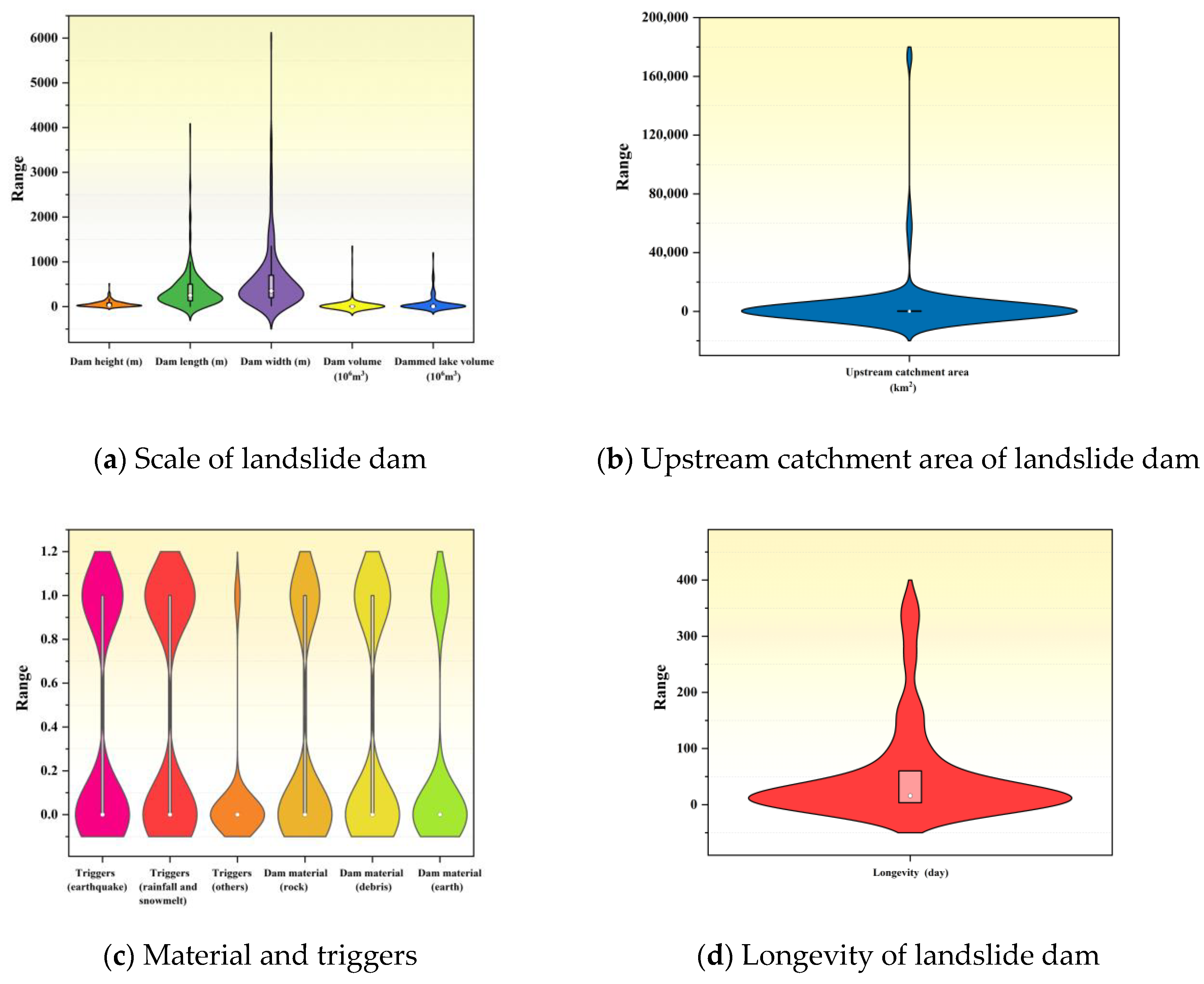
Longevity (day)	86.94	4.12	370	0.01	53.80	16.00	369.99

demonstrates the statistical analysis of the populated database for each metric (i.e., standard deviation (STD), kurtosis (Kurt), maximum, mean, median, and range).

The study used violin plots (Figure 4) to visualize key variables such as geometric characteristics, upstream catchment, triggering factors, dam materials, and lifespan of the weir dams in order to reveal the characteristics of their data distribution and variability.

As can be seen in Figure 4, the analysis of the geometric characteristics of the weir dams (dam height, dam length, dam width, dam volume, and water storage volume) shows that the dam width has the widest distribution with a large variability, while the data for the dam volume and the water storage volume are more concentrated, suggesting that they are relatively less variable. The distribution of dam height and length is relatively compact, though some outliers indicate significant differences in height and length among weirs. Secondly, in terms of upstream catchment area, the data distribution shows significant right skewness, with most weirs having small catchment areas, but a few very large dams exist, creating a long-tail effect and reflecting the heterogeneity of catchment sizes. The data are concentrated in the lower range, while a few extreme values result in long tails, whose impact on predictions needs to be considered in the modeling. For triggers and dam materials, the distribution of rainfall and snowmelt triggers is more dispersed, while the values of seismic triggers are relatively concentrated but with large variability, suggesting a large uncertainty in the impact of earthquake-induced weirs. In terms of dam materials, the distribution of rock and debris materials is more concentrated, while the distribution of soil materials is wider, reflecting the differences in the physical properties of different dam materials. The distribution of the weir lifetime variable is right skewed, with most weirs having shorter lifetimes and only a few dams having longer lifetimes. The main data are concentrated in the lower lifetime range, while the extreme values lead to a long-tail effect, indicating that the lifetime of weir dams is influenced by a number of factors and has a high degree of uncertainty.

Overall, these violin plots clearly show the concentration trend, the degree of variability, and the extreme values of the variables, which provide data support for the feature extraction, data preprocessing, and predictive modeling of the subsequent models. At the same time, these charts reflect the possible correlations between different variables, which need to be explored in depth in the modeling process.

3.4. Correlation Analysis

Correlation analysis, as a statistical approach [37], is used to evaluate the linear connection between two variables. The results are usually expressed in terms of correlation coefficient. By calculating the correlation coefficients between the parameters, the interactions and dependencies between the parameters can be understood, which in turn reduces the risk of model overfitting. In this study, the Pearson correlation coefficient is used to explore the correlation between model parameters, and the calculation formula is shown in Equation (37):

$$r_{XY}={\displaystyle \frac{{\displaystyle \sum _{k=1}^N(A_k-\overline{A})(B_k-\overline{B})}}{\sqrt{{\displaystyle \sum _{k=1}^N{(A_k-\overline{A})}^2{\displaystyle \sum _{k=1}^N{(B_k-\overline{B})}^2}}}}}$$

(37)

where $\overline{A}$ and $\overline{B}$ are the mean of $N$ test values, respectively, and $r_{XY}\in [0,1]$.

Figure 5 shows the correlation between different indicators. Among them, the dam volume shows high correlation with the dam height, length, and width, with correlation sizes of 0.73, 0.62, and 0.68 respectively, indicating that as the dam height increases, the other geometrical dimensions of the dam usually increase accordingly. In addition, the correlation between the dam volume and the weir volume is more significant, reaching 0.54, showing that the water storage capacity of the dam is closely related to its size. The correlation between the upstream catchment area and the weir volume is 0.46, which indicates that the catchment size has some influence on the dam storage capacity. Overall, the weir life is jointly influenced by a variety of factors, among which the dam geometry has a high predictive value, while the trigger factors and dam materials have relatively little influence on the life. The results of the above analysis can provide an important feature selection basis for the subsequent weir dam life prediction model.

4. Results

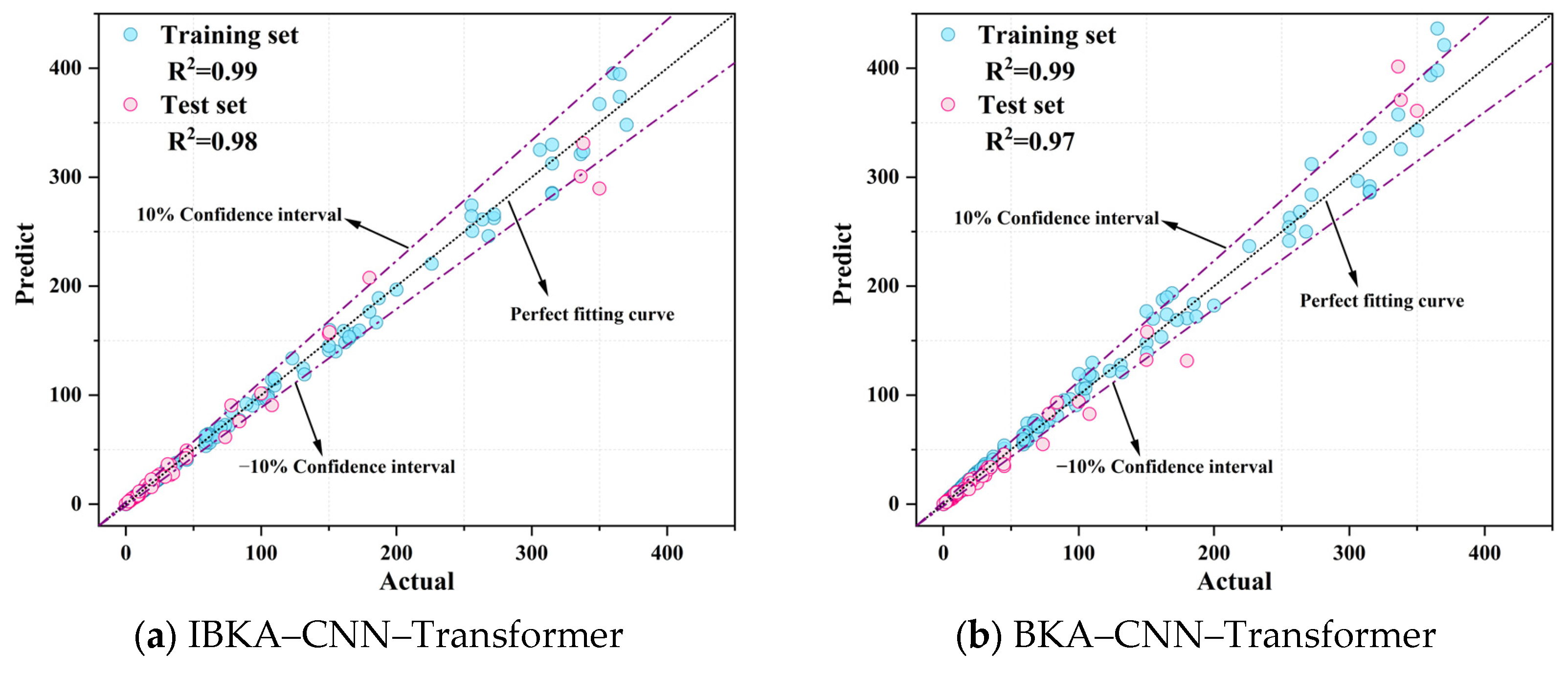
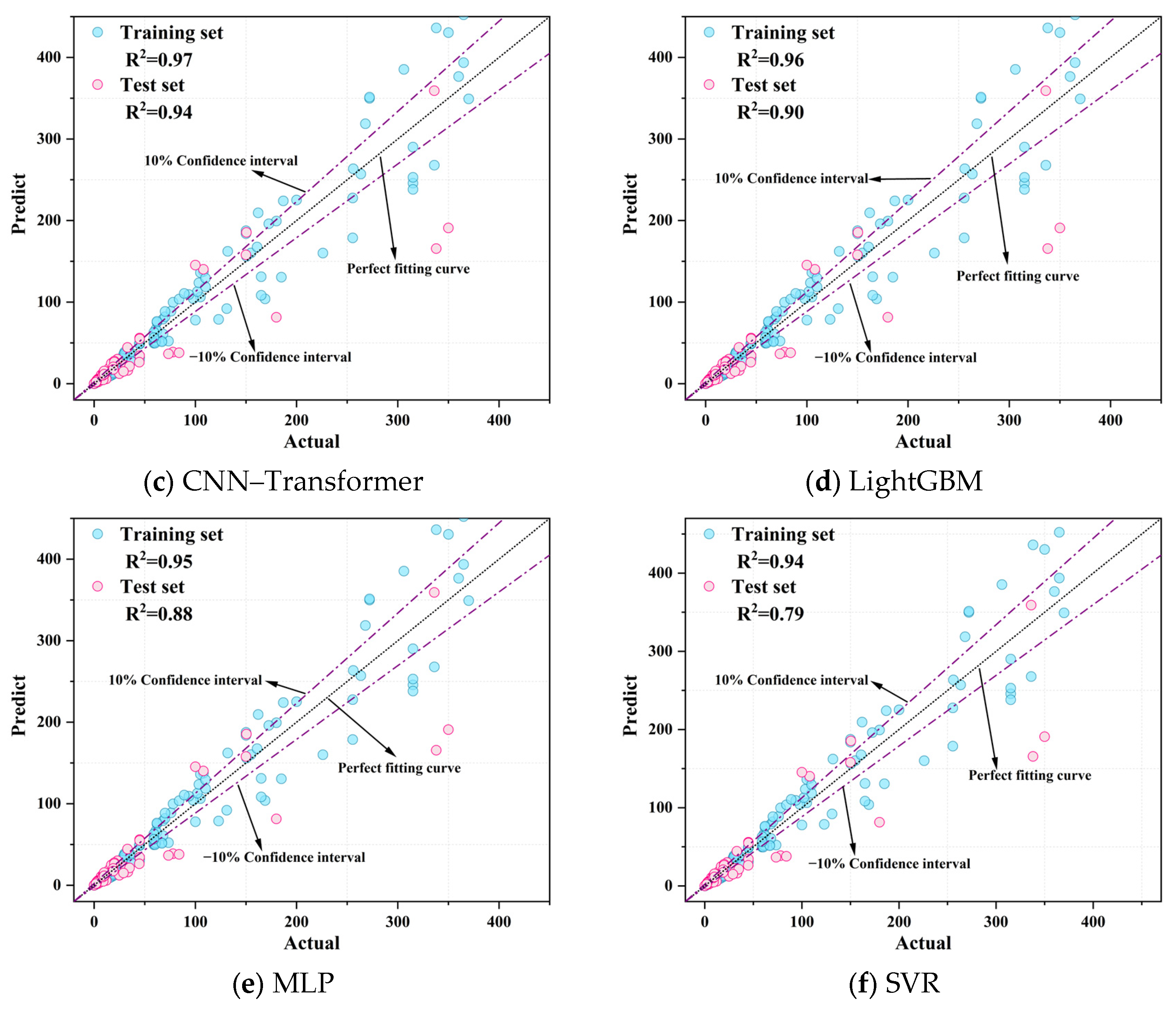
4.1. Presentation and Analysis of Prediction Results

In an attempt to verify the effectiveness of the six intelligent prediction models constructed for predicting the weir life, as well as to explore the performance advantages and disadvantages of each model in comparison, this section systematically compares and analyzes the prediction results of different models from two levels, namely, the training set and the test set. The fitting relationship between the predicted and actual values of each model is demonstrated through intuitive visual graphs, and the prediction accuracy and generalization ability of the models are further quantified by combining the key evaluation indexes.

As can be seen in Figure 6, the IBKA–CNN–Transformer model has the best performance, with R² of 0.99 and 0.98 for the training set and test set, respectively, showing very high fitting accuracy and excellent generalization ability. The BKA–CNN–Transformer model is the second best, with R² of 0.99 and 0.97 for the training set and test set, respectively, and with only a small deviation in the test set. The predicted and actual values are highly consistent with each other, with only a small deviation in the test set. CNN–Transformer performs slightly worse than the first two models, but its test set R² still reaches 0.94, indicating that it is able to effectively capture the nonlinear features in the data. In contrast, the prediction performance of the traditional machine-learning models is relatively weak. LightGBM and MLP have R² of 0.95 and 0.95 on the training set, but their R² on the test set drop to 0.90 and 0.88, respectively, with some of the predicted values deviating from the actual values. SVR has the most limited performance, with R² of 0.94 and 0.79 on the training and test sets, respectively, with significantly large errors, especially on the test set. SVR has the most limited performance, with R² of 0.94 and 0.79 in the training and test sets, respectively, and the error is significantly large, especially in the test set, where there are more points that deviate from the “perfect fit curve”. Overall, the deep-learning models outperform the traditional models in terms of prediction accuracy and generalization ability, especially the IBKA–CNN–Transformer, which shows excellent performance in all the indicators, proving its applicability and advantages in solving this research problem.

4.2. Model Performance Evaluation and Comparison

The study quantitatively evaluates the self-prediction performance of each model based on the prediction results of multiple models and selects the deterministic coefficient (R²), the adjusted deterministic coefficient (Adj.R²), the mean absolute percentage error (MAPE), the mean absolute error (MAE), the root-mean-square error (RMSE), and the variance accounted for (VAF), a total of six statistical indexes, to evaluate the comprehensive performance of each model. The generalization ability of the models is reflected more comprehensively and objectively by these indicators. Equations (38)–(43) are the mathematical definitions of these indicators [38,39].

R² measures the ability of the model to explain the target variable and takes the value of [0,1].

$$R^2=1-{\displaystyle \frac{{\displaystyle {\sum }_{i=1}^n{(y_i-{\widehat{y}}_i)}^2}}{{\displaystyle {\sum }_{i=1}^n{(y_i-{\overline{y}}_i)}^2}}}$$

(38)

where $y_i$ is the actual value, ${\widehat{y}}_i$ is the predicted value, $\overline{y}$ is the mean of the actual value, and $n$ is the number of data points.

Adj.R² takes into account the effect of the number of independent variables on R².

$$Adj.R^2=1-{\displaystyle \frac{(1-R^2)(n-1)}{n-k-1}}$$

(39)

where $k$ is the number of independent variables.

MAPE is used to measure the percentage of prediction error relative to the actual value with the formula

$$MAPE={\displaystyle \frac{1}{n}}{\displaystyle \sum _{i=1}^n\left|\frac{y_i-{\widehat{y}}_i}{y_i}\right|}\times 100\%$$

(40)

MAE is the average of the absolute values of all prediction errors:

$$MAE={\displaystyle \frac{1}{n}}{\displaystyle \sum _{i=1}^n\left|y_i-{\widehat{y}}_i\right|}$$

(41)

The RMSE reflects the mean square error between the predicted and actual values and is given by the following formula:

$$RMSE=\sqrt{{\displaystyle \frac{1}{n}}{\displaystyle \sum _{i=1}^n{(y_i-{\widehat{y}}_i)}^2}}$$

(42)

VAF is an indicator of variance explanatory power with the formula

$$VAF=(1-{\displaystyle \frac{Var(y_i-{\widehat{y}}_i)}{Var(y_i)}})\times 100\%$$

(43)

where Var denotes the variance.

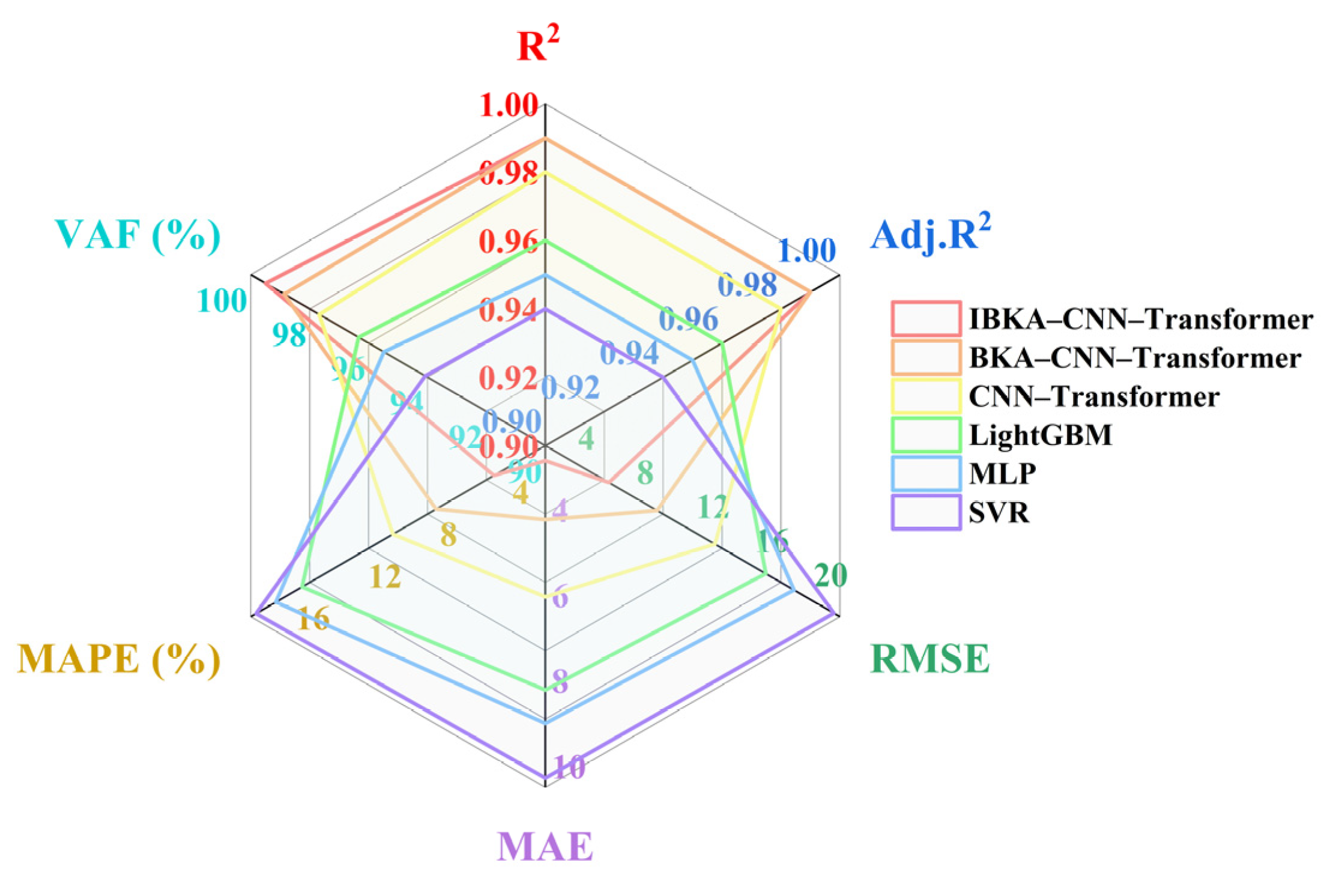
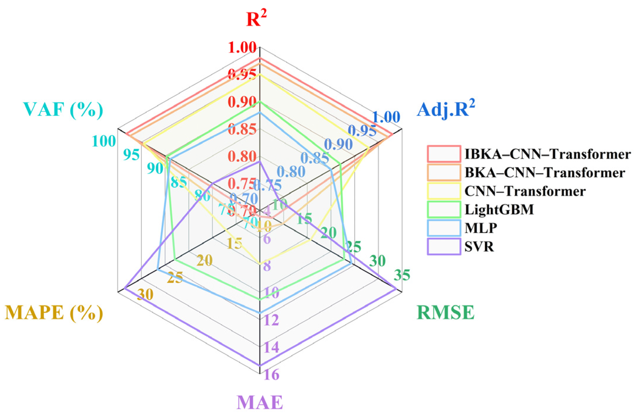
Radar diagrams are plotted based on the results of the calculations of the predictive performance of each model in

Table 2. Error comparison of models based on different imputation methods.

	Models	R2	Adj.R2	RMSE	MAE	MAPE	VAF (%)
Training Sets	IBKA–CNN–Transformer	0.99	0.99	6.32	2.85	4.85	99.50
	BKA–CNN–Transformer	0.99	0.99	9.59	4.23	8.05	98.87
	CNN–Transformer	0.98	0.98	13.52	6.04	10.44	97.68
	LightGBM	0.96	0.96	16.97	8.22	15.47	96.34
	MLP	0.95	0.95	18.89	9.00	16.91	95.48
	SVR	0.94	0.94	21.59	10.28	18.01	94.08
Testing Sets	IBKA–CNN–Transformer	0.98	0.98	10.58	4.45	9.93	98.21
	BKA–CNN–Transformer	0.97	0.97	12.69	5.39	11.71	97.38
	CNN–Transformer	0.95	0.93	18.36	7.92	14.73	94.53
	LightGBM	0.90	0.87	25.20	10.54	23.36	89.70
	MLP	0.88	0.85	26.67	11.53	26.27	88.91
	SVR	0.79	0.74	35.80	15.40	31.83	79.97

and are shown in Figure 7 and Figure 8.

The performance evaluation results from both the training and test sets indicate that the IBKA–CNN–Transformer and BKA–CNN–Transformer models exhibit significant advantages across all metrics. Specifically, the IBKA–CNN–Transformer achieves R² and VAF values of 0.99 and 99.50%, respectively, on the training set, and it maintains 0.98 and 98.21% on the test set. Additionally, its RMSE, MAE, and MAPE values are significantly lower than those of other models, demonstrating its high predictive accuracy and generalization capability. The BKA–CNN–Transformer performs slightly less effectively than the former but still achieves R² and VAF values of 0.97 and 97.38%, respectively, on the test set, outperforming other comparative models. In contrast, traditional models (such as LightGBM, MLP, and SVR) show acceptable performance on the training set but experience a significant decline on the test set, with R² and VAF dropping below 0.90 and 90%, respectively. Their error metrics (RMSE, MAE, MAPE) also increase notably, indicating weaker generalization capabilities and a tendency to overfit.

The superior performance of the IBKA–CNN–Transformer model is largely due to the advantages of the Transformer structure in multi-dimensional feature extraction and complex relationship modeling. In particular, the multi-head self-attention mechanism is able to efficiently capture the global dependencies between multi-dimensional input features and mine their potential higher-order interaction patterns by assigning dynamic attention weights to each input feature. This mechanism is able to extract feature representations from multiple subspaces in parallel, which makes the model performance more flexible and robust in the face of complex nonlinear data. The feed-forward neural network module further enhances the feature representation capability through nonlinear transformation, enabling the model to capture complex and implicit feature patterns in the input data. At the same time, residual concatenation and layer normalization ensure the stability of the deep network during the training process, effectively mitigating the gradient vanishing problem. These features enable the Transformer model to achieve a significant improvement in global modeling capability, and combined with the local feature extraction advantage of the CNN module, it strengthens the comprehensiveness and accuracy of feature learning. In addition, the model significantly improves the global exploration ability and local optimization accuracy of hyperparameter search by introducing the improved BKA optimization algorithm (IBKA), which achieves a better parameter combination during model training and effectively enhances the fitting ability and generalization performance of the model.

In summary, the IBKA–CNN–Transformer demonstrates stronger adaptability and robustness in complex data prediction tasks, making it a suitable candidate as the preferred model. Future research will focus on further optimization and refinement of the model to enhance its predictive accuracy and broaden its applicability.

4.3. SHAP-Based Analysis and Its Practical Implications

In order to explain the decision-making mechanism of the weir life intelligent prediction model in the prediction task and to quantify the influence of each input feature on the prediction results, the SHAP (SHapley Additive exPlanations) method was used in this study for feature importance analysis [40,41].

4.3.1. SHAP-Based Feature Importance Analysis

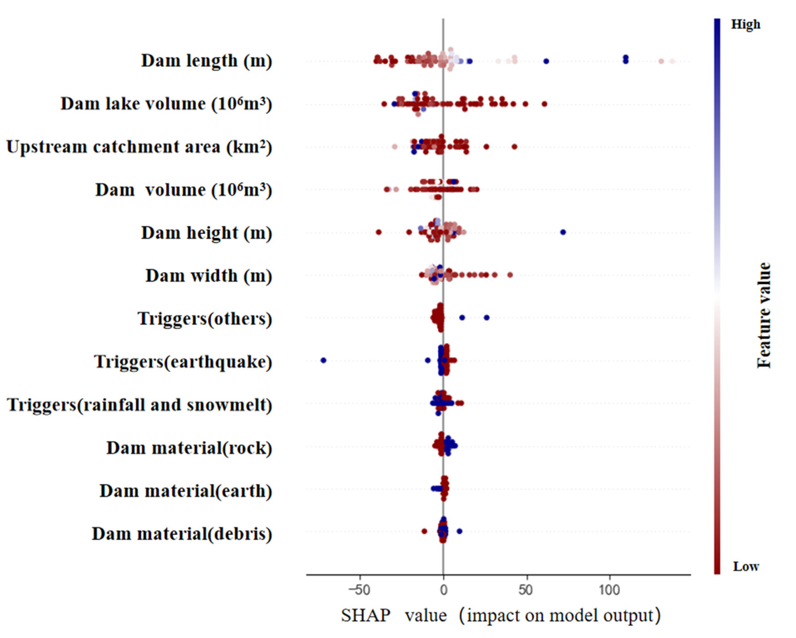
When processing numerical data in the CNN–Transformer model, the features first go through the CNN’s convolution and pooling operations to extract the local features, and then the global features are captured by the Transformer to capture the relationship between the global features; therefore, when SHAP is used to interpret the model, it acts directly on the deep feature layer, and the results reflect only the CNN–Transformer processed features’ contribution, which cannot be directly related to the original input features. At this point, reverse engineering needs to be introduced to map the importance of the deep features back to the original input space by restoring the feature extraction process of the CNN.

Specifically, reverse engineering requires layer-by-layer reverse operation for the CNN part: use transpose convolution to gradually restore the feature map extracted from the convolutional layer, use up-sampling to restore the dimensionality reduction operation after pooling, and finally, decode the feature contribution of each layer to the input feature space step by step. For the Transformer part, the global feature interactions are incorporated into the interpretation using the feature weights recorded by its attention mechanism. In this way, the importance of deep features can be reasonably redistributed to the original numerical features, combining global and local interpretations to completely reflect the model’s prediction logic. This approach reflects both the local pattern-capturing ability of CNN and incorporates the global feature modeling of Transformer, which helps to explain more intuitively the complex model’s dependence on the raw data and the basis for decision making. The analysis results are shown in Figure 9.

The detailed analysis of feature importance not only enhances the interpretability of the model, but also provides strong support for data processing and model optimization in regression prediction tasks. The application of this method proves the applicability and effectiveness of SHAP in the interpretation of complex deep-learning models. Figure 10 shows a comparison of the degree of contribution of different influencing factors to the weir life, which is based on SHAP analysis and highlights the differences between the characteristic importance of different factors.

In the process of predicting the lifespan of landslide dams, the importance of each feature exhibits significant variation. Figure 10 visually demonstrates the degree of influence of each feature on the prediction results through the height of the rectangles, accompanied by a quantitative representation. A taller rectangle indicates that the corresponding feature contributes more substantially to the prediction outcome, while a shorter rectangle suggests a lesser influence. This visualization method clearly highlights the relative importance of different features within the model, offering valuable insights into the key drivers behind the prediction results.

As can be seen in the figure, dam length is the most important feature in the model predictions, contributing 26.9% to the results, showing the critical influence of the weir length on its lifetime. Dam lake volume (DLV) is the next most important feature, contributing 20.7%, indicating that the amount of water that a weir can hold significantly affects its lifetime. Upstream catchment area and dam volume contribute 11.3% and 9.6%, respectively, to the model, showing the significant influence of hydrology and dam structure on weir life. Dam height and dam width contribute 8.6% and 8.0% to the model, respectively, indicating that although they are not as important to the model as dam length and storage volume in terms of their predictive ability, they are still important structural parameters affecting longevity. Trigger factors also have some influence on the weir life: the “other” trigger (others) contributes 3.8%; the earthquake trigger (earthquake) and rainfall trigger (rainfall and snowmelt) contribute 3.4% and 2.7%, respectively, indicating that natural events are important external factors affecting weir life. Material-related features (dam material) contribute less to the predicted results, indicating that material properties have a weaker direct effect on weir life than the geometric features of the dam and the natural conditions.

The importance of the scale of the dam and the upstream catchment area is further amplified in the nested figure. The scale of the dam is the main driver, with a contribution value of 73.8%. This suggests that the influence of dam size far outweighs other characteristics in the study of weir life. Natural triggers (earthquakes and rainfall) have some degree of influence on weir life, but the effect is weak compared with weir size. Material properties have a smaller effect on the model but cannot be completely ignored, especially in cases where different material combinations may affect stability.

4.3.2. Implications of SHAP Results for Landslide Dam Management

The SHAP-based feature importance analysis provides valuable interpretability to the predictive model by quantifying the influence of individual features on landslide dam lifespan prediction. The results indicate that dam length and dammed lake volume are the most critical factors affecting lifespan prediction, which aligns with traditional engineering perspectives—larger dams with higher storage capacities tend to exhibit more complex stability dynamics. However, a notable new insight revealed by SHAP analysis is the significant influence of the upstream catchment area, which was previously considered secondary to geometric and material properties in many empirical models. The high SHAP value for upstream catchment area suggests that hydrological factors play a more dominant role than expected, particularly in regions where rainfall-induced erosion significantly impacts dam stability.

This finding has important implications for landslide dam risk assessment and management strategies. Given the strong impact of upstream catchment area, future monitoring and risk evaluation should incorporate detailed hydrological assessments rather than relying predominantly on dam geometry and material composition alone. Additionally, the relatively lower SHAP values of triggering factors such as earthquakes and rainfall suggest that while these external forces are crucial for dam formation and sudden failures, their effect on long-term stability may be less dominant than internal structural factors. This insight can guide prioritization of mitigation strategies, emphasizing structural reinforcement and sediment control measures over purely event-driven risk mitigation.

Furthermore, the transparent ranking of feature contributions through SHAP analysis enables adaptive dam management policies. For example, regions with a high upstream catchment impact may require enhanced flood regulation infrastructure, while areas primarily influenced by geomorphological factors may focus more on stabilization engineering measures. By integrating data-driven feature importance insights, SHAP analysis refines existing landslide dam assessment models, allowing for more targeted and proactive risk management strategies. These results highlight the potential of SHAP analysis not only as a tool for improving model interpretability but also as a foundation for practical engineering decision making.

5. Discussion

5.1. Model Performance Advantages and Limitations

The IBKA–CNN–Transformer model proposed in this study exhibits outstanding prediction performance, with coefficients of determination (R²) of 0.99 and 0.98 for the training and test sets, respectively, demonstrating its effectiveness in predicting weir life. This performance improvement is largely attributed to the hybrid structure of the model. The CNN module excels at capturing intrinsic patterns in geometric attributes through its powerful local feature extraction capabilities, while the Transformer module accurately models global features and long-range dependencies using the multi-head self-attention mechanism. Additionally, the enhanced IBKA algorithm optimizes the model’s hyperparameters, improving its adaptability and generalization to complex nonlinear data. The introduction of SHAP analysis further enhances model interpretability by quantifying the contributions of key features to predictions, providing a clear basis for identifying the primary drivers of weir life.

However, despite its strong performance, the model exhibits high computational complexity and significant training costs, particularly when handling large-scale datasets. Although the IBKA algorithm mitigates overfitting in deep-learning models with small sample sizes to some extent, the model still relies heavily on data volume and quality. Moreover, the model’s reliance on geometric features and hydrological conditions may lead to performance degradation when key features are missing, which warrants careful consideration in practical applications.

The model accounts for several critical factors influencing the stability and longevity of landslide dams, including hydrological conditions, material properties, and triggering factors such as rainfall, earthquakes, and extreme weather events. However, the potential impact of shock waves from seismic activity is not explicitly included in the model. These shock waves, especially from large-scale seismic events, can significantly affect dam stability and trigger landslides, representing a limitation of the current model. Additionally, while the model considers extreme weather as a triggering factor, the broader impacts of climate change, including long-term shifts in environmental conditions, have not been fully integrated. This remains another limitation that could be addressed in future versions of the model, particularly to better capture the cumulative effects of extreme weather patterns over time.

5.2. Role of SHAP Method in Model Training

In this study, the introduction of the SHAP method not only enhances the interpretability of the model, but also provides strong support for feature selection and optimization. The SHAP method makes the decision-making process of the model more transparent by quantifying the marginal contribution of each feature to the model prediction and revealing the importance of the key variables such as the dam length, the storage volume, and the area of the upstream catchment area in the prediction of weir life. The results of this analysis provide a clear, data-driven direction for optimizing the input feature set by adjusting the weights of features based on their importance as determined by SHAP values. Features with higher SHAP values receive more weight in the model, enhancing their influence on the predictions. This optimization process improves model training efficiency by focusing on the most relevant features while reducing the impact of less important features. The clarity of the optimization direction was measured by evaluating the improvements in model performance after adjusting feature weights. In addition, the SHAP approach further advances the model’s ability to understand complex data patterns by revealing the interactions between features, thus theoretically enhancing the model’s prediction performance. More importantly, this method provides a quantitative basis for practical engineering applications; e.g., by identifying the significant influence of dam size, it can provide scientific support for resource allocation and management decisions in weir design and maintenance. Therefore, the SHAP method is not only a powerful tool for model interpretation, but also an important means to guide data processing and to optimize the modeling process, which can provide valuable experience for the construction and optimization of complex prediction models.

6. Conclusions

This study provides an efficient, accurate, and interpretable solution for weir life prediction by improving the model, introducing the SHAP method, and implementing multi-scale feature modeling. The following conclusions were drawn:

(1) The study collected and organized 297 sets of data on weir dam lifespan, constructing a comprehensive sample database. By selecting 12 key factors affecting weir dam lifespan as predictive indicators, the correlations between these factors were analyzed, and the degree of correlation was quantified. The results reveal a significant correlation between the geometric characteristics of weir dams (e.g., dam height, dam length, dam width) and hydrological conditions (e.g., water storage volume, upstream catchment area), with correlation coefficients of 0.73, 0.62, and 0.68, respectively. This analysis provides a scientific basis for the selection and optimization of features in subsequent models.

(2) An Improved Black-Winged Kite Algorithm (IBKA) is proposed to optimize the hyperparameters of the CNN–Transformer hybrid model. The IBKA algorithm significantly enhances the global search ability and local optimization accuracy by introducing a dynamic adaptive mechanism, population clustering strategy, and dynamic migration strategy. Compared with the traditional BKA algorithm, the IBKA dynamically adjusts the learning rate and migration probability based on the adaptation degree during the iteration process, effectively avoiding the loss of population diversity and local optimization issues. Experimental results demonstrate that the IBKA algorithm exhibits superior adaptability and stability in complex, high-dimensional optimization problems. Specifically, when handling nonlinear features in weir life prediction, it rapidly converges to the global optimal solution, significantly improving the prediction accuracy and generalization ability of the model.

(3) Based on the improved IBKA algorithm, the CNN–Transformer hybrid model constructed in this study demonstrates exceptional performance in the weir life prediction task. Experimental results indicate that the model achieves a coefficient of determination (R²) of 0.99 and 0.98 on the training and test sets, respectively, significantly outperforming traditional machine-learning models (e.g., LightGBM, MLP, and SVR) and other deep-learning models (e.g., CNN–Transformer and BKA–CNN–Transformer). The superiority of this model is primarily attributed to its combination of the local feature extraction capability of CNN and the global feature modeling capability of Transformer. The CNN module efficiently captures local patterns of weir geometric features through convolution and pooling operations, while the Transformer module captures complex interactions among global features through the multi-head self-attention mechanism. Furthermore, the optimization of the model hyperparameters by the IBKA algorithm further enhances its adaptability and generalization ability in complex nonlinear data. This improved model provides an efficient and accurate solution for weir life prediction with broad application potential.

(4) By introducing the SHAP (SHapley Additive exPlanations) method, this study significantly improves the interpretability of the model and quantifies the contribution of key features to weir life prediction. The analysis results indicate that the geometric characteristics and hydrological conditions of weir dams are the primary drivers of their lifespan. Specifically, dam length contributes the most to the prediction, at 26.9%, followed by dam lake volume, at 20.7%. Upstream catchment area and dam volume contribute 11.3% and 9.6%, respectively, highlighting the significant influence of hydrological conditions and dam structure on lifespan. In contrast, triggers (e.g., earthquake and rainfall) contribute less, with the earthquake trigger and the rainfall and snowmelt trigger contributing only 3.4% and 2.7%, respectively. Dam materials (e.g., rock, debris, and earth materials) contribute the least, indicating a weak direct effect of material properties on lifespan. The SHAP method not only enhances the transparency of the model but also provides strong support for feature selection and optimization, helping to identify the key features that contribute most to the prediction results. This analysis provides a scientific basis for the design, maintenance, and risk assessment of weir dams and enhances the credibility of the model in practical engineering applications.

In summary, the IBKA–CNN–Transformer model proposed in this study provides an efficient, accurate, and interpretable solution for weir life prediction. The results not only offer a scientific basis for weir risk assessment and disaster prevention but also open new avenues for the application of intelligent prediction technology in complex system modeling. However, there is still room for improvement in the computational efficiency and the performance of the model in small-sample scenarios. Future research will focus on further optimizing the computational performance of the algorithm and exploring how to integrate domain knowledge with data-driven models to address diverse challenges in practical engineering applications, thereby promoting the widespread adoption of intelligent prediction techniques in geohazard management.