Development of Enhanced Stress Prediction Models for Fixed Traffic Loads on Flexible Pavements Based on Response Surface Methodology (RSM) and Machine Learning (ML) Techniques

Abstract

Pavement design is influenced by traffic load, which affects its lifespan. Traditional methods classify traffic load into fixed traffic, fixed vehicle, variable traffic, and vehicle/axle loads. In fixed traffic, pavement thickness is based on the maximum expected wheel load without considering load repetitions. Meanwhile, in fixed vehicle scenarios, it is calculated by the repetitions of a standard axle load. For nonstandard axle loads, the equivalent axle load is determined by multiplying repetitions by the corresponding equivalent load factor. In variable traffic, each axle and its repetitions are analyzed independently. This study proposes enhanced models for fixed traffic loads, focusing on single, dual, and tridem axles in a single-layer pavement model, to improve stress prediction accuracy. The results show that a quadratic model with a base-10 logarithmic transformation accurately predicts stresses. Additionally, machine learning models, especially Gradient Boosting, provided more accurate predictions than traditional models, with lower mean squared error (MSE) and root mean squared error (RMSE). The results show that these models are effective in predicting the stress in pavement. These findings provide valuable insights that can lead to better pavement design and more effective maintenance practices.

1. Introduction

There are several major factors that lead to the deterioration of asphalt pavement, and traffic loads are among the most important. These loads significantly affect pavement performance due to their repetition over time [1,2]. Traffic loads, their frequency, and the resulting stresses are pivotal in determining the performance and longevity of the pavement. When vehicles pass, they generate different stresses that can cause various types of damage, depending on the type and weight of the load. As the weight of the load increases, the likelihood of pavement damage also increases, leading to deformation, cracking, and fatigue.

Pavements are designed to withstand a certain number of load repetitions throughout their service life; however, excessive repetition of heavy loads can exceed the structural capacity of the pavement [3,4,5]. Each time a vehicle passes over the pavement, it generates stress that accumulates over time, which can lead to fatigue failure, especially in areas with heavy traffic. Moreover, determining the stresses generated by vehicles in pavements poses a significant challenge for designers. This process involves understanding how different types of vehicles, loads, and traffic patterns affect pavement performance. Therefore, understanding and addressing these factors is essential for maintaining the safety and longevity of asphalt pavements [6,7,8].

The impact of traffic and vehicles on pavement design can be classified into three main categories: fixed traffic, fixed vehicle, and variable vehicle and traffic. In fixed traffic scenarios, pavement thickness is determined based on the load of a single wheel, disregarding the number of load repetitions [9,10]. However, in situations involving different types of wheels, such as heavy wheel loads on highway pavements, they need to be converted to an equivalent single-wheel load (ESWL). Conversely, the fixed vehicle method considers the number of load repetitions of a standard axle, typically a single axle with dual tires and a load of 18 kips (80 kN). For pavements exposed to various axle types, like tandem or tridem axles, they are converted to an equivalent axle load factor (EALF) to achieve an equivalent effect based on an 18 kip (80 kN) single-axle load [11,12].

The variable traffic and vehicles method treats vehicles and traffic separately, eliminating the need to assign equivalent factors for different axles. This method evaluates strains and deflections for each load individually. Several methods have been developed to determine the equivalent single-wheel load (ESWL), including the equal vertical stress criterion, equal vertical deflection criterion, equal tensile strain criterion, criterion based on equal contact pressure, and criterion based on equivalent contact radius. The semi-rational equal vertical stress criterion, introduced by Boyd and Foster [10,13], calculates the produced stress (ESWL) based on pavement layer thickness.

However, safety concerns arose from accelerated traffic tests, leading to the equal vertical deflection criterion by Foster and Ahlvin [10,14]. This method assumes a homogeneous half-space pavement layer and determines the developed vertical deflection at the top of the subgrade layer using Boussinesq solutions. Huang, 1969 [15], suggested that this method still poses safety risks, as some pavement thicknesses exceed those obtained by the Boyd and Foster method. Other methods, such as the criterion based on equal contact pressure and the criterion based on equivalent contact radius, have been developed to address these challenges.

Previous methods are ineffective in explaining the stress concentration generated by tire contact overlap in tandem and tridem axles, resulting in an incomplete understanding of stress distribution. However, the thickness of pavement layers plays a crucial role in load distribution; thicker layers help minimize stress on underlying layers and enhance the ability to support loads. Likewise, axle configuration, in terms of tire spacing, has a significant effect on how stress is distributed. Greater spacing between tires minimizes overlap stresses, while closely spaced tires increase stress overlap [16,17,18,19]. These challenges show the need for advanced modeling tools like PITRA PAVE.

PITRA PAVE is a tool used to study pavement performance by analyzing how it responds to structural stresses induced by traffic loads. It contains a wide variety of materials, including asphalt mixtures, granular layers, and subgrade. The tool models multiple load configurations, including single, dual, and multi-axle loads, while accounting for dynamic loading conditions. Furthermore, PITRA PAVE enables for wide assessments of stress, strain, and deflection within pavement layers. This provides important information on the long-term performance of pavement infrastructure. Moreover, PITRAPAVE offers advanced functions, including dynamic loading simulations and better material analysis. These advancements enable for a more thorough understanding of pavement behavior under complex loading situations, surpassing earlier tools like KENPAVE [20,21,22].

In addition to PITRA PAVE, response surface methodology (RSM) is widely used to model the performance of pavements. RSM applies statistical tools to investigate correlations between variables like layer thickness and tire spacing, predicting pavement behavior under load [23,24]. RSM provides valuable insights, however, it has its limitations. It struggles to capture complex, nonlinear interactions and manage the large datasets common in real-world pavement systems [25,26]. This is where machine learning (ML) starts to assist the development of models. Unlike RSM, which relies on predetermined mathematical assumptions, ML algorithms can evaluate enormous datasets, find nonlinear patterns, and generate predictions without simplifications. Integrating ML into the modeling process provides for more precise and trustworthy pavement performance forecasts, leading to better assessments of long-term pavement behavior [27,28].

This research aims to develop models to improve stress prediction in flexible pavements under fixed traffic conditions. A homogeneous single-layer model was adopted to isolate the effects of axle configuration (single, tandem, tridem), tire spacing, and pavement thickness, avoiding the complexity of multi-layer systems. Response surface methodology (RSM) has been used to model stresses from single, tandem, and tridem axles. To further enhance the accuracy of these models, machine learning (ML) was integrated, enabling more precise predictions by analyzing complex patterns.

2. Methods

In this study, the PITRA PAVE v1.0.0 tool was used to evaluate the stress caused by different axle configurations, including single, tandem, and tridem axles. However, The analysis focused on a homogeneous, linear-elastic, isotropic single-layer pavement model with a layer thickness ranging from 0 to 50 inches in 5-inch increments. The tire load was set at 4500 lb, and the tire pressure was maintained at 100 psi, while the elastic modulus and Poisson’s ratio were kept constant at 10,000 psi and 0.5, respectively. According to the outputs from PITRA PAVE, vertical stress is primarily influenced by pavement thickness rather than by the elastic modulus or Poisson’s ratio. However, the tire pressure was fixed at 100 psi, as variations minimally affect vertical stress, and load was set at 4500 lb because vertical stress scales linearly with load. Stresses were measured at multiple locations, as illustrated in Figure 1, to identify the critical stress point and adopt it for the analysis and model development. For the single axle, tandem axle, and tridem axles, the tire spacings in the Y direction were set to 7, 14, and 21 inches, respectively. In the X direction, spacings for the tandem and tridem axles were 24, 48, and 72 inches. Subsequently, Design-Expert V.13 was employed to develop prediction models for the stresses produced by the different axle types. The models considered pavement thickness and tire spacing in both the X and Y directions, with the response variable being the developed critical stresses.

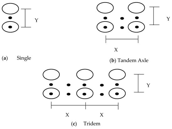
Figure 1. Locations of stress measurements.

Machine Learning Approach for Stress Prediction Modeling

In this study, a machine learning approach was employed to optimize and assess several regression models for predicting stress values in single, tandem, and tridem axles. The procedure began by loading the dataset and applying preprocessing steps, such as a log transformation to the target variable (stress) to stabilize its variance. The dataset was then divided into training and testing subsets, with 80% used for training and 20% for testing and evaluation. Various regression models were trained, including linear regression, ridge, lasso, support vector regression (SVR), decision tree, random forest, gradient boosting, LightGBM, and CATBoost. To improve model performance, polynomial features were added. The models were evaluated using performance metrics like mean squared error (MSE), R², mean absolute error (MAE), and root mean squared error (RMSE). The best-performing model was chosen based on these metrics. Additionally, to assess model interpretability and feature significance, diagnostics such as residual plots and Shapley Additive Explanations (SHAP) analysis were performed. The results were visualized to provide a better understanding of the model’s performance. A flowchart summarizing the entire process is shown in Figure 2.

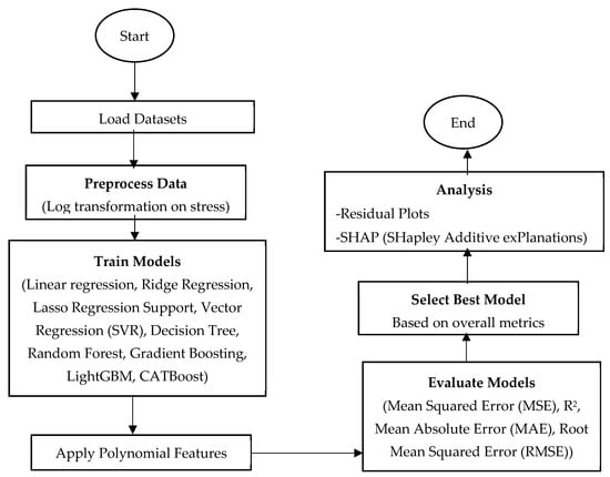
Figure 2. Flow chart of machine leaning approach.

3. Analysis and Results

3.1. RSM Results for Single, Tandem, and Tridem Axles

This section analyzes the data produced by response surface methodology (RSM) for several axle configurations, including single, tandem, and tridem.

3.1.1. Single Axle with Dual Tires

Table 1 provides a comprehensive summary of the outputs generated by the PITRA PAVE v1.0.0 software. The data indicate that, as the depth of the assessment points increases, the values of the stresses exhibit a significant decline. This trend highlights the relationship between depth and stress distribution within the pavement structure, emphasizing the importance of considering depth in the design and analysis of pavement systems. Moreover, the analysis reveals that reduced spacing between tires correlates with increased stress levels. This phenomenon can be attributed to stress overlap, where closely spaced tires distribute their load over a smaller area, resulting in higher localized stress concentrations. Understanding this relationship is crucial for optimizing tire configurations to minimize pavement damage. Further, to investigate the interactions between tire spacing (in the Y direction), pavement thickness, and the resultant stress response, a statistical evaluation was conducted using response surface methodology (RSM). This approach allowed for the development of a predictive model that assesses stress at various depths within the pavement layer. Importantly, a base 10 logarithmic transformation was applied to the data to enhance the model’s performance, as preliminary analyses indicated that the untransformed model did not yield satisfactory results. Table 2 presents the fit summary of the various models generated during this analysis. Notably, the quadratic model emerged as the most effective predictor of stress, supported by its significant p-value and superior adjusted and predicted R² values when compared to alternative models. In contrast, the cubic model was found to be aliased, suggesting that it may not provide reliable predictions within the studied parameters.

Table 1. Outputs of PITRA PAVE for single axle with dual tires.

Run	Y Spacing (A) (in)	Thickness (B) (in)	Stress (psi)	Run	Y Spacing (A) (in)	Thickness (B) (in)	Stress (psi)
1	14	0	100.03	18	7	30	4.5288
2	14	5	49.749	19	7	35	3.3682
3	14	10	19.733	20	7	40	2.5941
4	14	15	11.376	21	7	45	2.0524
5	14	20	7.8512	22	7	50	1.6592
6	14	25	5.5819	23	21	0	100.24
7	14	30	4.1164	24	21	5	49.372
8	14	35	3.1359	25	21	10	18.528
9	14	40	2.4537	26	21	15	9.4982
10	14	45	1.9623	27	21	20	5.9935
11	14	50	1.5986	28	21	25	4.5274
12	7	0	178.14	29	21	30	3.5376
13	7	5	61.325	30	21	35	2.8012
14	7	10	29.161	31	21	40	2.2553
15	7	15	15.742	32	21	45	1.8459
16	7	20	9.5875	33	21	50	1.534
17	7	25	6.3817

Table 2. Fit summary of the various models for single axle with dual tires.

Fit Summary
Source	Sequential p-Value	Adjusted R2	Predicted R2	Performance
Linear	<0.0001	0.9197	0.9047
2FI	0.4196	0.9188	0.892
Quadratic	<0.0001	0.9903	0.9862	Suggested
Cubic	<0.0001	0.9973	0.9953	Aliased

Table 3 presents the ANOVA results for the quadratic model. The analysis reveals that the impact of tire spacing alone on the model is insignificant, as indicated by a p-value greater than 0.05. Conversely, the effect of pavement thickness is significant, with a p-value below 0.05, showing its importance in stress response. Additionally, the interaction between pavement thickness and tire spacing was found to be significant. This is because, at depths close to the surface, there is no overlap between stresses but, as the location of analysis goes deeper, there will be an overlap between the developed stresses from the tires. Table 3 also summarizes the model’s fit statistics. Notably, the difference between the adjusted and predicted R² values is less than 2, indicating strong agreement between the predicted and observed values. The adequate precision value of 76, which far exceeds the threshold of 4, further suggests that the model is not only effective but also capable of reliably navigating the design space, making it a valuable tool for engineers in pavement design. Figure 3 illustrates several important diagnostic plots for the quadratic model: the normal probability plot, residuals versus predicted values, residuals versus run, and predicted versus actual values. The normal probability plot is particularly useful for assessing the distribution of residuals; a straight line on this plot indicates a favorable fit for linear regression. Any deviations from this line, such as right or left skewness, could suggest potential issues with the model’s assumptions about error distribution [29,30]. To assess homoscedasticity, the assumption that the variance of errors is constant across all levels of the independent variables, externally studentized residuals were plotted against predicted values. A scatter plot with symmetrically shaped errors around zero supports the assumption of homoscedasticity, whereas any asymmetric patterns would indicate heteroscedasticity [31]. Figure 3 demonstrates a symmetrical pattern around zero, confirming the model’s suitability for accurately predicting the developed stresses. The residuals versus run number plot is instrumental in detecting autocorrelation among disturbances. The absence of autocorrelation is indicated by residuals transitioning randomly between positive and negative values, as observed in Figure 3. This randomness suggests that the stresses are well modeled by the independent variables [32]. However, the actual versus predicted values plot provides a visual representation of the model’s predictive capability. Figure 3 shows a strong correlation between actual and predicted values, with data points closely aligning with the 1:1 line. This alignment underscores the model’s accuracy in predicting developed stresses under various loading conditions, validating its utility in pavement design. Equation (1) describes the quadratic model.

$${\sigma }_z={10}^{(2.31928-0.026869\ast A-0.072919\ast B+0.000267\ast A\ast B+0.000387\ast A^2+0.000676\ast B^2)}\ast \left({\displaystyle \frac{tire load }{4500}}\right)$$

(1)

where:

• ${\sigma }_z$ = Vertical stress;
• A = spacing between tires in the Y direction;
• B = thickness of the pavement.

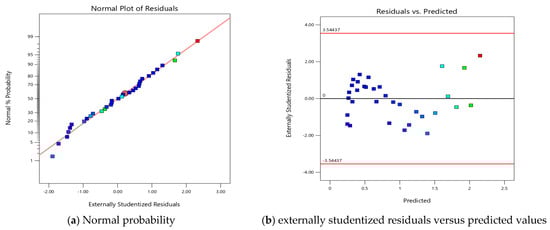
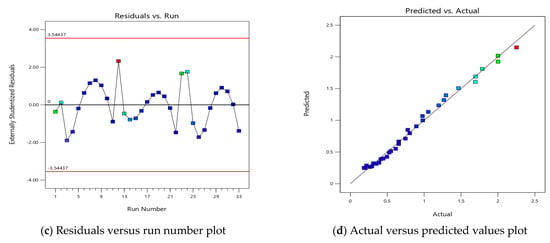
Figure 3. Plots analyzing the quadratic model of developed stress for single axle.

Table 3. ANOVA for quadratic model for single axle model.

Source	Sum of Squares	df	Mean Square	F-Value	p-Value	Performance
Model	11.19	5	2.24	651.13	<0.0001	significant
A-A	0	1	0	0.0035	0.9534
B-B	1.61	1	1.61	469.74	<0.0001
AB	0.0192	1	0.0192	5.58	0.0256
A2	0.0026	1	0.0026	0.7674	0.3887
B2	0.7346	1	0.7346	213.75	<0.0001
Residual	0.0928	27	0.0034
Cor Total	11.28	32
Fit statistics
Std. Dev.	0.0586		R2		0.9918
Mean	0.8933		Adjusted R2		0.9903
C.V. %	6.56		Predicted R2		0.9862
			Adeq Precision		76.0539

Table 3. ANOVA for quadratic model for single axle model.

Source	Sum of Squares	df	Mean Square	F-Value	p-Value	Performance
Model	11.19	5	2.24	651.13	<0.0001	significant
A-A	0	1	0	0.0035	0.9534
B-B	1.61	1	1.61	469.74	<0.0001
AB	0.0192	1	0.0192	5.58	0.0256
A2	0.0026	1	0.0026	0.7674	0.3887
B2	0.7346	1	0.7346	213.75	<0.0001
Residual	0.0928	27	0.0034
Cor Total	11.28	32
Fit statistics
Std. Dev.	0.0586		R2		0.9918
Mean	0.8933		Adjusted R2		0.9903
C.V. %	6.56		Predicted R2		0.9862
			Adeq Precision		76.0539

3.1.2. Tandem Axle with Dual Tires

The stresses induced by a tandem axle with dual tires were evaluated using the PITRA PAVE software. As shown in Table 4, the resulting stress values exhibit a clear decrease as the measurement depth increases. Additionally, the spacing between tires in both the Y and X directions plays a significant role in stress development. Specifically, reduced spacing tends to result in higher stress levels within a certain range. To better understand this relationship, a statistical analysis was performed using response surface methodology (RSM), focusing on the depth at which the stress was measured and the tire spacing. This method enabled the construction of a predictive model that effectively captures the complex dynamics of stress distribution. The use of a base 10 logarithmic transformation further enhanced the model’s accuracy by stabilizing variance and improving the overall fit. The fit summary provided in Table 5 suggests the use of a quadratic model, while the cubic model was excluded due to aliasing issues. The quadratic model was chosen because of its significant p-value and high adjusted R² value, both of which indicate a strong correlation between the key influencing factors and the response variable. The detailed ANOVA results for the quadratic model are shown in Table 6, underscoring the significant impact of both tire spacing and stress measurement depth on stress development, as evidenced by consistently low p-values below 0.05. Moreover, the fit statistics summarized in Table 6 reveal only a minimal difference between the adjusted and predicted R² values, which further confirms the model’s reliability. The adequate precision value, exceeding 4, reinforces the model’s robustness, making it a reliable tool for practical applications in pavement design.

$${\sigma }_z={10}^{(2.37052-0.067929\ast A-0.003682\ast B-0.026319\ast C-0.000087\ast A\ast B+0.000267\ast A\ast C-0.0000025\ast B\ast C+0.000706\ast A^2+0.000043\ast B^2+0.000379\ast C^2)}\ast \left({\displaystyle \frac{tire load }{4500}}\right)$$

(2)

where:

• ${\sigma }_z$ = Vertical stress;
• A = thickness of the pavement;
• B = spacing between tires in the X direction;
• C = spacing between tires in the Y direction.

Table 4. Outputs of PITRA PAVE for tandem axle with dual tires.

Run	Thickness (A) (in)	X Spacing (B) (in)	Y Spacing (C) (in)	Stress (psi)	Run	Thickness (A) (in)	X Spacing (B) (in)	Y Spacing (C) (in)	Stress (psi)
1	0	48	14	100.02	51	30	72	21	3.5763
2	5	48	14	49.751	52	35	72	21	2.8552
3	10	48	14	19.747	53	40	72	21	2.3253
4	15	48	14	11.42	54	45	72	21	1.9317
5	20	48	14	7.9388	55	50	72	21	1.6345
6	25	48	14	5.7221	56	0	48	21	100.24
7	30	48	14	4.3103	57	5	48	21	49.374
8	35	48	14	3.3781	58	10	48	21	18.541
9	40	48	14	2.735	59	15	48	21	9.5364
10	45	48	14	2.2721	60	20	48	21	6.0706
11	50	48	14	1.9268	61	25	48	21	4.6606
12	0	24	14	99.902	62	30	48	21	3.7227
13	5	24	14	49.798	63	35	48	21	3.0333
14	10	24	14	20.024	64	40	48	21	2.526
15	15	24	14	12.088	65	45	48	21	2.1453
16	20	24	14	8.8936	66	50	48	21	1.8521
17	25	24	14	6.8103	67	0	48	7	178.09
18	30	24	14	5.4004	68	5	48	7	61.327
19	35	24	14	4.3897	69	10	48	7	29.176
20	40	24	14	3.6312	70	15	48	7	15.788
21	45	24	14	3.0442	71	20	48	7	9.6781
22	50	24	14	2.5809	72	25	48	7	6.5263
23	0	72	14	100.08	73	30	48	7	4.7283
24	5	72	14	49.75	74	35	48	7	3.6167
25	10	72	14	19.735	75	40	48	7	2.8821
26	15	72	14	11.383	76	45	48	7	2.3688
27	20	72	14	7.8658	77	50	48	7	1.9938
28	25	72	14	5.6076	78	0	24	7	177.72
29	30	72	14	4.156	79	5	24	7	61.387
30	35	72	14	3.1912	80	10	24	7	29.525
31	40	72	14	2.5253	81	15	24	7	16.538
32	45	72	14	2.0499	82	20	24	7	10.729
33	50	72	14	1.7011	83	25	24	7	7.7046
34	0	72	7	170.46	84	30	24	7	5.8928
35	5	72	7	61.326	85	35	24	7	4.6858
36	10	72	7	29.163	86	40	24	7	3.8213
37	15	72	7	15.749	87	45	24	7	3.1724
38	20	72	7	9.6023	88	50	24	7	2.6707
39	25	72	7	6.4078	89	0	24	21	100.01
40	30	72	7	4.569	90	5	24	21	49.413
41	35	72	7	3.4242	91	10	24	21	18.772
42	40	72	7	2.6667	92	15	24	21	10.048
43	45	72	7	2.1411	93	20	24	21	6.8141
44	50	72	7	1.7629	94	25	24	21	5.618
45	0	72	21	100.3	95	30	24	21	4.702
46	5	72	21	49.373	96	35	24	21	3.9576
47	10	72	21	18.53	97	40	24	21	3.3561
48	15	72	21	9.5044	98	45	24	21	2.8682
49	20	72	21	6.007	99	50	24	21	2.47
50	25	72	21	4.5524

Table 4. Outputs of PITRA PAVE for tandem axle with dual tires.

Run	Thickness (A) (in)	X Spacing (B) (in)	Y Spacing (C) (in)	Stress (psi)	Run	Thickness (A) (in)	X Spacing (B) (in)	Y Spacing (C) (in)	Stress (psi)
1	0	48	14	100.02	51	30	72	21	3.5763
2	5	48	14	49.751	52	35	72	21	2.8552
3	10	48	14	19.747	53	40	72	21	2.3253
4	15	48	14	11.42	54	45	72	21	1.9317
5	20	48	14	7.9388	55	50	72	21	1.6345
6	25	48	14	5.7221	56	0	48	21	100.24
7	30	48	14	4.3103	57	5	48	21	49.374
8	35	48	14	3.3781	58	10	48	21	18.541
9	40	48	14	2.735	59	15	48	21	9.5364
10	45	48	14	2.2721	60	20	48	21	6.0706
11	50	48	14	1.9268	61	25	48	21	4.6606
12	0	24	14	99.902	62	30	48	21	3.7227
13	5	24	14	49.798	63	35	48	21	3.0333
14	10	24	14	20.024	64	40	48	21	2.526
15	15	24	14	12.088	65	45	48	21	2.1453
16	20	24	14	8.8936	66	50	48	21	1.8521
17	25	24	14	6.8103	67	0	48	7	178.09
18	30	24	14	5.4004	68	5	48	7	61.327
19	35	24	14	4.3897	69	10	48	7	29.176
20	40	24	14	3.6312	70	15	48	7	15.788
21	45	24	14	3.0442	71	20	48	7	9.6781
22	50	24	14	2.5809	72	25	48	7	6.5263
23	0	72	14	100.08	73	30	48	7	4.7283
24	5	72	14	49.75	74	35	48	7	3.6167
25	10	72	14	19.735	75	40	48	7	2.8821
26	15	72	14	11.383	76	45	48	7	2.3688
27	20	72	14	7.8658	77	50	48	7	1.9938
28	25	72	14	5.6076	78	0	24	7	177.72
29	30	72	14	4.156	79	5	24	7	61.387
30	35	72	14	3.1912	80	10	24	7	29.525
31	40	72	14	2.5253	81	15	24	7	16.538
32	45	72	14	2.0499	82	20	24	7	10.729
33	50	72	14	1.7011	83	25	24	7	7.7046
34	0	72	7	170.46	84	30	24	7	5.8928
35	5	72	7	61.326	85	35	24	7	4.6858
36	10	72	7	29.163	86	40	24	7	3.8213
37	15	72	7	15.749	87	45	24	7	3.1724
38	20	72	7	9.6023	88	50	24	7	2.6707
39	25	72	7	6.4078	89	0	24	21	100.01
40	30	72	7	4.569	90	5	24	21	49.413
41	35	72	7	3.4242	91	10	24	21	18.772
42	40	72	7	2.6667	92	15	24	21	10.048
43	45	72	7	2.1411	93	20	24	21	6.8141
44	50	72	7	1.7629	94	25	24	21	5.618
45	0	72	21	100.3	95	30	24	21	4.702
46	5	72	21	49.373	96	35	24	21	3.9576
47	10	72	21	18.53	97	40	24	21	3.3561
48	15	72	21	9.5044	98	45	24	21	2.8682
49	20	72	21	6.007	99	50	24	21	2.47
50	25	72	21	4.5524

Table 5. Fit summary of the various models for tandem axle with dual tires.

Source	Sequential p-Value	Adjusted R2	Predicted R2	Performance
Linear	<0.0001	0.9027	0.8962
2FI	0.2316	0.904	0.8904
Quadratic	<0.0001	0.9887	0.9869	Suggested
Cubic	<0.0001	0.9971	0.9962	Aliased

Table 5. Fit summary of the various models for tandem axle with dual tires.

Source	Sequential p-Value	Adjusted R2	Predicted R2	Performance
Linear	<0.0001	0.9027	0.8962
2FI	0.2316	0.904	0.8904
Quadratic	<0.0001	0.9887	0.9869	Suggested
Cubic	<0.0001	0.9971	0.9962	Aliased

Table 6. ANOVA for quadratic model for tandem axle model.

Source	Sum of Squares	df	Mean Square	F-Value	p-Value	Performance
Model	30.07	9	3.34	951.31	<0.0001	significant
A-A	2.41	1	2.41	684.99	<0.0001
B-B	0.0547	1	0.0547	15.58	0.0002
C-C	0.0583	1	0.0583	16.6	0.0001
AB	0.0726	1	0.0726	20.66	<0.0001
AC	0.0574	1	0.0574	16.36	0.0001
BC	7.8 × 10−6	1	7.8 × 10−6	0.0022	0.9626
A2	2.4	1	2.4	684.32	<0.0001
B2	0.0135	1	0.0135	3.85	0.053
C2	0.0076	1	0.0076	2.16	0.1451
Residual	0.3126	89	0.0035
Cor Total	30.38	98
Fit statistics
Std. Dev.	0.0593			R2	0.9897
Mean	0.9337			Adjusted R2	0.9887
C.V. %	6.35			Predicted R2	0.9869
				Adeq Precision	100.3383

Table 6. ANOVA for quadratic model for tandem axle model.

Source	Sum of Squares	df	Mean Square	F-Value	p-Value	Performance
Model	30.07	9	3.34	951.31	<0.0001	significant
A-A	2.41	1	2.41	684.99	<0.0001
B-B	0.0547	1	0.0547	15.58	0.0002
C-C	0.0583	1	0.0583	16.6	0.0001
AB	0.0726	1	0.0726	20.66	<0.0001
AC	0.0574	1	0.0574	16.36	0.0001
BC	7.8 × 10−6	1	7.8 × 10−6	0.0022	0.9626
A2	2.4	1	2.4	684.32	<0.0001
B2	0.0135	1	0.0135	3.85	0.053
C2	0.0076	1	0.0076	2.16	0.1451
Residual	0.3126	89	0.0035
Cor Total	30.38	98
Fit statistics
Std. Dev.	0.0593			R2	0.9897
Mean	0.9337			Adjusted R2	0.9887
C.V. %	6.35			Predicted R2	0.9869
				Adeq Precision	100.3383

Figure 4 shows the residual plots for the quadratic model, including the normal probability plot, residuals versus predicted values, residuals versus run, and actual versus predicted values. These plots are crucial for evaluating the model’s performance through the assumptions. The normal probability plot is specifically used to assess the distribution of the residuals. As seen in Figure 4, the residuals are close to a straight line, indicating that the errors are normally distributed. This alignment suggests that the quadratic model is well suited for the data. Homoscedasticity, which refers to the assumption of equal variance across the range of predicted values, is examined through the plot of externally studentized residuals versus predicted values. As depicted in Figure 4, the residuals are symmetrically distributed around zero, with no apparent pattern or systematic deviation. This symmetry indicates that the model’s predictions are consistent across the range of data. Autocorrelation can undermine the model’s effectiveness by indicating that the residuals are not independent, which is another key assumption for regression models. In Figure 4, the residuals appear to transition randomly between positive and negative values, with no discernible pattern. This randomness suggests that there is no autocorrelation, meaning the stresses are well captured by the independent variables in the model. Finally, the plot of actual versus predicted values demonstrates the model’s predictive accuracy. As shown in Figure 3, the data points closely align along the 1:1 line, indicating a strong correlation between the actual values and the values predicted. The strong agreement between actual and predicted values indicates the model’s ability to predict accurately.

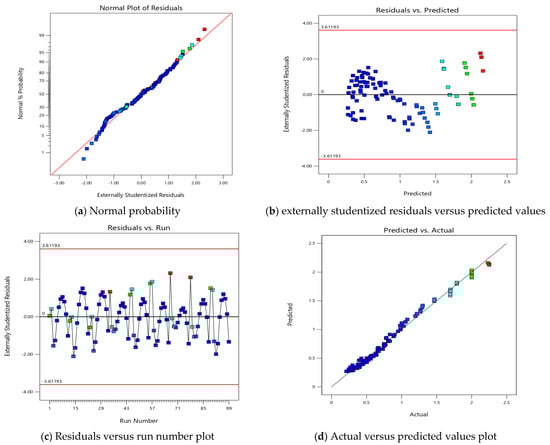
Figure 4. Plots analyzing the quadratic model of developed stress for tandem axle with dual tires.

3.1.3. Tridem Axle with Dual Tires

The stress of a tridem axle with dual tires was analyzed using the PITRA PAVE software. As shown in Table 7, with increasing depth, the stresses generated by the loads decrease significantly. The distance between the tires in both the Y and X directions plays a significant role in the stress levels. The smaller the distance, the greater the stress. To identify this relationship, a statistical analysis was conducted using response surface methodology (RSM). This analysis aims to develop a predictive relationship for stress based on loads, pavement depth, and tire spacing. A base 10 logarithmic transformation was applied to enhance model accuracy by stabilizing variance. This is because, without the transformation, the performance of the models was poor. The fit summary in Table 8 shows that the quadratic model is suggested, while the cubic model is rejected. The quadratic model’s significant p-value and high adjusted R² indicate a strong correlation between tire spacing, depth, and stress response. The ANOVA results listed in Table 9 describe the significant influence of tire spacing and measurement depth on stress development, with p-values consistently below 0.05. Additionally, the fit statistics in Table 7 show a minimal difference between the adjusted and predicted R² values. The adequate precision value, exceeding 4, indicates the reliability of the model. Equation (3) shows the quadratic model.

$${\sigma }_z={10}^{(2.40058-0.064288\ast A-0.026072\ast B-0.005825\ast C+0.000268\ast A\ast B-0.000149\ast A\ast C-0.000013\ast B\ast C+0.000725\ast A^2+0.000386\ast B^2+0.00007\ast C^2)}\ast \left({\displaystyle \frac{tire load }{4500}}\right)$$

(3)

• ${\sigma }_z$ = Vertical stress;
• A = thickness of the pavement;
• B = spacing between tires in the Y direction;
• C = spacing between tires in the X direction.

Table 7. Outputs of PITRA PAVE for tridem axle with dual tires.

Run	Thickness (A) (in)	Y Spacing (B) (in)	X Spacing (C) (in)	Stress (psi)	Run	Thickness (A) (in)	Y Spacing (B) (in)	X Spacing (C) (in)	Stress (psi)
1	0	14	48	100.01	51	30	7	24	7.2569
2	5	14	48	49.753	52	35	7	24	6.0035
3	10	14	48	19.761	53	40	7	24	5.0484
4	15	14	48	11.464	54	45	7	24	4.2924
5	20	14	48	8.0264	55	50	7	24	3.6822
6	25	14	48	5.8623	56	0	7	72	178.28
7	30	14	48	4.5041	57	5	7	72	61.326
8	35	14	48	3.6203	58	10	7	72	29.165
9	40	14	48	3.0163	59	15	7	72	15.756
10	45	14	48	2.582	60	20	7	72	9.6171
11	50	14	48	2.2551	61	25	7	72	6.4339
12	0	14	24	99.892	62	30	7	72	4.6093
13	5	14	24	49.846	63	35	7	72	3.4803
14	10	14	24	20.314	64	40	7	72	2.7392
15	15	14	24	12.19	65	45	7	72	2.2298
16	20	14	24	9.9359	66	50	7	72	1.8666
17	25	14	24	8.0387	67	0	21	48	100.24
18	30	14	24	6.6843	68	5	21	48	49.376
19	35	14	24	5.6434	69	10	21	48	18.553
20	40	14	24	4.8087	70	15	21	48	9.5746
21	45	14	24	4.1261	71	20	21	48	6.1478
22	50	14	24	3.5631	72	25	21	48	4.7939
23	0	14	72	100.13	73	30	21	48	3.9077
24	5	14	72	49.75	74	35	21	48	3.2654
25	10	14	72	19.737	75	40	21	48	2.7967
26	15	14	72	11.39	76	45	21	48	2.4446
27	20	14	72	7.8803	77	50	21	48	2.1702
28	25	14	72	5.6333	78	0	21	24	100.01
29	30	14	72	4.1956	79	5	21	24	49.454
30	35	14	72	3.2464	80	10	21	24	19.016
31	40	14	72	2.5968	81	15	21	24	10.598
32	45	14	72	2.1374	82	20	21	24	7.6348
33	50	14	72	1.8035	83	25	21	24	6.7086
34	0	7	48	178.04	84	30	21	24	5.8664
35	5	7	48	61.329	85	35	21	24	5.1141
36	10	7	48	29.192	86	40	21	24	4.4569
37	15	7	48	15.833	87	45	21	24	3.8905
38	20	7	48	9.7687	88	50	21	24	3.4061
39	25	7	48	6.671	89	0	21	72	100.31
40	30	7	48	4.9277	90	5	21	72	49.373
41	35	7	48	3.8652	91	10	21	72	18.531
42	40	7	48	3.17	92	15	21	72	9.5074
43	45	7	48	2.6853	93	20	21	72	6.0139
44	50	7	48	2.3283	94	25	21	72	4.5659
45	0	7	24	177.67	95	30	21	72	3.5971
46	5	7	24	61.449	96	35	21	72	2.8845
47	10	7	24	29.89	97	40	21	72	2.3635
48	15	7	24	17.333	98	45	21	72	1.9789
49	20	7	24	11.871	99	50	21	72	1.6903
50	25	7	24	9.0275

Table 7. Outputs of PITRA PAVE for tridem axle with dual tires.

Run	Thickness (A) (in)	Y Spacing (B) (in)	X Spacing (C) (in)	Stress (psi)	Run	Thickness (A) (in)	Y Spacing (B) (in)	X Spacing (C) (in)	Stress (psi)
1	0	14	48	100.01	51	30	7	24	7.2569
2	5	14	48	49.753	52	35	7	24	6.0035
3	10	14	48	19.761	53	40	7	24	5.0484
4	15	14	48	11.464	54	45	7	24	4.2924
5	20	14	48	8.0264	55	50	7	24	3.6822
6	25	14	48	5.8623	56	0	7	72	178.28
7	30	14	48	4.5041	57	5	7	72	61.326
8	35	14	48	3.6203	58	10	7	72	29.165
9	40	14	48	3.0163	59	15	7	72	15.756
10	45	14	48	2.582	60	20	7	72	9.6171
11	50	14	48	2.2551	61	25	7	72	6.4339
12	0	14	24	99.892	62	30	7	72	4.6093
13	5	14	24	49.846	63	35	7	72	3.4803
14	10	14	24	20.314	64	40	7	72	2.7392
15	15	14	24	12.19	65	45	7	72	2.2298
16	20	14	24	9.9359	66	50	7	72	1.8666
17	25	14	24	8.0387	67	0	21	48	100.24
18	30	14	24	6.6843	68	5	21	48	49.376
19	35	14	24	5.6434	69	10	21	48	18.553
20	40	14	24	4.8087	70	15	21	48	9.5746
21	45	14	24	4.1261	71	20	21	48	6.1478
22	50	14	24	3.5631	72	25	21	48	4.7939
23	0	14	72	100.13	73	30	21	48	3.9077
24	5	14	72	49.75	74	35	21	48	3.2654
25	10	14	72	19.737	75	40	21	48	2.7967
26	15	14	72	11.39	76	45	21	48	2.4446
27	20	14	72	7.8803	77	50	21	48	2.1702
28	25	14	72	5.6333	78	0	21	24	100.01
29	30	14	72	4.1956	79	5	21	24	49.454
30	35	14	72	3.2464	80	10	21	24	19.016
31	40	14	72	2.5968	81	15	21	24	10.598
32	45	14	72	2.1374	82	20	21	24	7.6348
33	50	14	72	1.8035	83	25	21	24	6.7086
34	0	7	48	178.04	84	30	21	24	5.8664
35	5	7	48	61.329	85	35	21	24	5.1141
36	10	7	48	29.192	86	40	21	24	4.4569
37	15	7	48	15.833	87	45	21	24	3.8905
38	20	7	48	9.7687	88	50	21	24	3.4061
39	25	7	48	6.671	89	0	21	72	100.31
40	30	7	48	4.9277	90	5	21	72	49.373
41	35	7	48	3.8652	91	10	21	72	18.531
42	40	7	48	3.17	92	15	21	72	9.5074
43	45	7	48	2.6853	93	20	21	72	6.0139
44	50	7	48	2.3283	94	25	21	72	4.5659
45	0	7	24	177.67	95	30	21	72	3.5971
46	5	7	24	61.449	96	35	21	72	2.8845
47	10	7	24	29.89	97	40	21	72	2.3635
48	15	7	24	17.333	98	45	21	72	1.9789
49	20	7	24	11.871	99	50	21	72	1.6903
50	25	7	24	9.0275

Table 8. Fit summary of the various models for tridem axle with dual tires.

Source	Sequential p-Value	Adjusted R2	Predicted R2	Performance
Linear	<0.0001	0.883	0.8753
2FI	0.044	0.8893	0.8737
Quadratic	<0.0001	0.9859	0.9838	Suggested
Cubic	<0.0001	0.9964	0.9952	Aliased

Table 8. Fit summary of the various models for tridem axle with dual tires.

Source	Sequential p-Value	Adjusted R2	Predicted R2	Performance
Linear	<0.0001	0.883	0.8753
2FI	0.044	0.8893	0.8737
Quadratic	<0.0001	0.9859	0.9838	Suggested
Cubic	<0.0001	0.9964	0.9952	Aliased

Table 9. ANOVA for quadratic model for tridem axle model.

Source	Sum of Squares	df	Mean Square	F-Value	p-Value	Performance
Model	27.93	9	3.1	763.87	<0.0001	significant
A-A	2.52	1	2.52	620.06	<0.0001
B-B	0.0591	1	0.0591	14.54	0.0003
C-C	0.1624	1	0.1624	39.98	<0.0001
AB	0.0582	1	0.0582	14.33	0.0003
AC	0.2107	1	0.2107	51.86	<0.0001
BC	0.0002	1	0.0002	0.0495	0.8244
A2	2.54	1	2.54	624.05	<0.0001
B2	0.0079	1	0.0079	1.94	0.1672
C2	0.0354	1	0.0354	8.71	0.0041
Residual	0.3616	89	0.0041
Cor Total	28.29	98
Fit statistics
Std. Dev.	0.0637			R2	0.9872
Mean	0.9651			Adjusted R2	0.9859
C.V. %	6.6			Predicted R2	0.9838
				Adeq Precision	92.953

Table 9. ANOVA for quadratic model for tridem axle model.

Source	Sum of Squares	df	Mean Square	F-Value	p-Value	Performance
Model	27.93	9	3.1	763.87	<0.0001	significant
A-A	2.52	1	2.52	620.06	<0.0001
B-B	0.0591	1	0.0591	14.54	0.0003
C-C	0.1624	1	0.1624	39.98	<0.0001
AB	0.0582	1	0.0582	14.33	0.0003
AC	0.2107	1	0.2107	51.86	<0.0001
BC	0.0002	1	0.0002	0.0495	0.8244
A2	2.54	1	2.54	624.05	<0.0001
B2	0.0079	1	0.0079	1.94	0.1672
C2	0.0354	1	0.0354	8.71	0.0041
Residual	0.3616	89	0.0041
Cor Total	28.29	98
Fit statistics
Std. Dev.	0.0637			R2	0.9872
Mean	0.9651			Adjusted R2	0.9859
C.V. %	6.6			Predicted R2	0.9838
				Adeq Precision	92.953

Figure 5 shows the residual plots of the quadratic model. These plots shown in Figure 5 include the normal probability plot, residuals versus predicted values, residuals versus run number, and actual versus predicted values. However, these plots describe how well the model fits the data and predicts the stress accurately. The normal probability plot is essential for assessing whether the residuals, or errors, follow a normal distribution. The data points on this plot should form a straight line, indicating that the residuals are normally distributed. As seen in Figure 5, the residuals are close to the theoretical line, suggesting that the data are normally distributed. Furthermore, the plot of externally studentized residuals versus predicted values is used to evaluate the reliability of the model. This plot is crucial for assessing homoscedasticity, which refers to the assumption that the error terms (the differences between the observed and predicted values of the dependent variable) have equal variance across all levels of the independent variables. As seen in Figure 5, the residuals are symmetrically distributed around zero, showing no clear pattern or trend. The residuals versus run number plot is used to detect any autocorrelation among the residuals, which would suggest that the errors are not independent. It can be seen in Figure 5 that the residuals transition randomly between positive and negative values, indicating that there is no unsystematic pattern. This randomness suggests that there is no autocorrelation, indicating that the model accurately describes the relationship between the independent variables and the stresses. On the other hand, the plot of actual versus predicted values illustrates the model’s accuracy in predicting the observed values. As noted in Figure 5, the data points closely follow the 1:1 line, indicating a strong correlation between the actual values and those predicted by the model. This close alignment proves the model’s effectiveness in predicting the developed stresses.

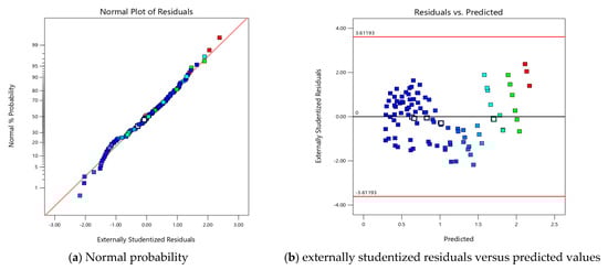
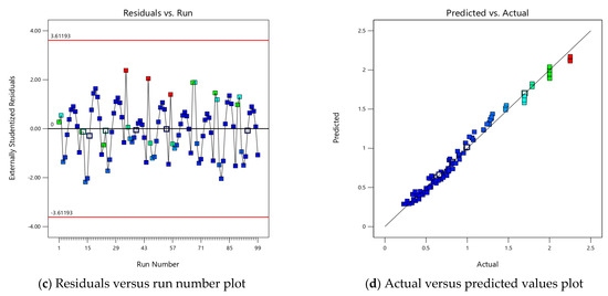
Figure 5. Plots analyzing the quadratic model of developed stress for tridem axle with dual tires.

3.2. Performance Analysis of Machine Learning Models

This section evaluates the performance of various machine learning models in predicting stress levels for single, tandem, and tridem axles.

3.2.1. Machine Learning Model Performance for Single Axle Stress Prediction

Table 10 displays the performance of different regression models. The results indicate that gradient boosting is the top performer, with the lowest testing MSE (0.006061), RMSE (0.077851), and a high R² value of 0.971168, demonstrating its strong ability to generalize to new data. Likewise, random forest performs well, with low testing MSE (0.016694) and RMSE (0.129204), and a solid R² of 0.920587. However, the decision tree model overfits the training data, obtaining desirable outcomes on the training set (MSE: 0, R²: 1, MAE: 0, RMSE: 0) but struggling with testing data (MSE: 0.020817, R²: 0.900970, MAE: 0.124350, RMSE: 0.144282). The huge disagreement between its training and testing performance indicates it is memorizing the training data instead of learning general patterns. Both linear and ridge regression illustrate uniform results, with ridge slightly beating linear regression on the testing data. On the other hand, lasso regression displays considerable underfitting, with high errors and a negative R² value for testing. LightGBM’s performance is insufficient, with large errors in both training and testing. Meanwhile, CatBoost performs moderately. In summary, gradient boosting is the most dependable model. To further confirm the efficiency of gradient boosting, diagnostic plots were studied as shown in Figure 6. The Q-Q plot demonstrated that the residuals follow a normal distribution, verifying the model’s correctness. The actual vs. predicted plot also indicated strong alignment, reflecting the model’s predictive reliability. Additionally, the externally studentized residuals plot confirmed there was no bias, and the residuals vs. run number plot indicated that the model’s predictions were not influenced by the sequence of the data. These diagnostics together prove gradient boosting as an effective and stable model. Figure 7 presents Shapley Additive Explanations (SHAP) values for the parameters of the thickness and spacing. Thickness (B) has a considerably greater average impact on predictions, which results in noticeable variances in outcomes. Otherwise, Y spacing demonstrates a more consistent and uniform effect, contributing uniformly across different cases.

Table 10. Performance of different regression models for single axle.

Model	Training MSE	Testing MSE	Training R2	Testing R2	Training MAE	Testing MAE	Training RMSE	Testing RMSE
Linear Regression	0.016519	0.011680	0.989721	0.944439	0.109154	0.091461	0.128526	0.108072
Ridge Regression	0.019780	0.008936	0.987692	0.957490	0.112288	0.074093	0.140640	0.094531
Lasso Regression	1.185774	0.741216	0.262126	−2.52603	0.932521	0.789881	1.088932	0.860939
Decision Tree	0.000000	0.020817	1.000000	0.900970	0.000000	0.124350	0.000000	0.144282
Random Forest	0.005351	0.016694	0.996670	0.920587	0.057087	0.089123	0.073151	0.129204
Gradient Boosting	0.000007	0.006061	0.999996	0.971168	0.001996	0.055807	0.002672	0.077851
LightGBM	1.607014	1.075682	0.000000	−4.11712	1.088507	0.930306	1.267680	1.037151
CatBoost	0.000011	0.014862	0.999993	0.929300	0.002677	0.115107	0.003276	0.121910

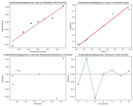
Figure 6. Residuals plots analyzing gradient boosting regression model for single axle.

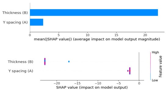
Figure 7. SHAP value analysis for single axle model features.

3.2.2. Machine Learning Model Performance for Tandem Axle Stress Prediction

The results shown in Table 11 illustrate the performance of different regression models, with gradient boosting showing as the best model. It shows the lowest testing MSE (0.001118), MAE (0.023510), and RMSE (0.033436), with a near-perfect R² value of 0.999367, demonstrating excellent accuracy and generalization. Random forest likewise works well, with low testing errors (MSE: 0.005714, R²: 0.996763) and negligible overfitting. Decision tree, however, displays evidence of overfitting, attaining excellent training results (MSE: 0, R²: 1) but inadequate testing performance (MSE: 0.012414, R²: 0.992966). Linear and ridge regression produce consistent results with high R² values (0.990983 and 0.990604, respectively), although ridge slightly follows linear. Furthermore, lasso regression struggles with severe underfitting, indicated in its large testing errors (MSE: 1.702942, R²: 0.035162). LightGBM and CatBoost perform well during training but demonstrate poor generalization ability on testing data. Therefore, gradient boosting is the most dependable model. In addition, the gradient boosting model is further validated by diagnostic plots, as shown in Figure 8. The Q-Q plot indicates that the residuals are regularly distributed, confirming the assumption of normality. The actual vs. predicted values plot illustrates a good correlation between predicted and actual values, presenting high predictive accuracy. The externally studentized residuals vs. predicted values plot indicates no bias, confirming the absence of systematic mistakes in the model. Finally, the residuals vs. run number plot indicates that the model’s predictions are independent of the data point sequence, ensuring stability. Overall, gradient boosting stands out as the most dependable model, supported by consistent performance across all evaluation metrics. However, the SHAP value analysis in Figure 9 displays that the thickness of the pavement has the most significant impact on model predictions, as confirmed by its high average SHAP value. Otherwise, X spacing and Y spacing show lesser average affects, with Y spacing demonstrating a more consistent influence.

Table 11. Performance of different regression models for tandem axle.

Model	Training MSE	Testing MSE	Training R2	Testing R2	Training MAE	Testing MAE	Training RMSE	Testing RMSE
Linear Regression	0.017564	0.015914	0.985709	0.990983	0.112486	0.100295	0.132530	0.126152
Ridge Regression	0.017797	0.016584	0.985520	0.990604	0.110984	0.101056	0.133406	0.128781
Lasso Regression	1.184310	1.702942	0.036404	0.035162	0.890889	1.113038	1.088260	1.304968
Decision Tree	0.000000	0.012414	1.000000	0.992966	0.000000	0.083175	0.000000	0.111420
Random Forest	0.001753	0.005714	0.998574	0.996763	0.031148	0.059024	0.041867	0.075589
Gradient Boosting	0.000021	0.001118	0.999983	0.999367	0.003692	0.023510	0.004535	0.033436
LightGBM	0.059909	0.098171	0.951256	0.944379	0.179682	0.257142	0.244764	0.313323
CatBoost	0.000005	0.042487	0.999996	0.975928	0.001702	0.111855	0.002162	0.206124

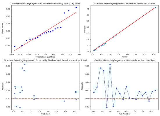
Figure 8. Residuals plots analyzing gradient boosting regression model for tandem axle.

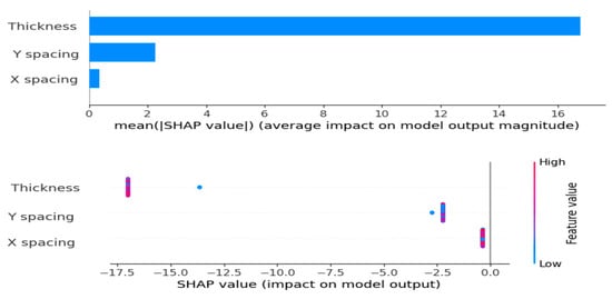
Figure 9. SHAP value analysis for tandem axle model features.

3.2.3. Machine Learning Model Performance for Tridem Axle Stress Prediction

The Table 12 demonstrates the performance of various regression models based on significant metrics. Gradient boosting is demonstrated as the best performer, with the lowest testing MSE (0.003260), MAE (0.037326), and RMSE (0.057093), as well as an almost perfect R² value of 0.998295, suggesting superior precision and generalization. Random forest also performs well, with a modest variation between training and testing results (MSE: 0.001837 vs. 0.013046, R²: 0.998324 vs. 0.993176), showing low overfitting. On the other hand, decision tree exhibits obvious overfitting, obtaining perfect training results (MSE: 0, R²: 1) but poorer testing performance (MSE: 0.014616, R²: 0.992354). Both linear regression and ridge regression perform consistently, with high R² values and low errors, albeit ridge marginally trails behind linear regression. Lasso regression faces significant challenges with severe underfitting, as shown by its high testing error (MSE: 1.913,948) and a negative R² value (−0.001202). While LightGBM and CatBoost perform well during training, their higher testing errors (MSE: 0.114631 and 0.115462, respectively) and lower R² values (0.940036 and 0.939601) suggest they struggle to generalize effectively to unseen data. To further test the efficiency of gradient boosting, diagnostic plots were employed to verify its accuracy, as shown in Figure 10. The normal probability plot (Q-Q Plot) demonstrates that the residuals follow a normal distribution with acceptable deviations. However, the actual vs. predicted values plot reveals significant alignment, showing good predictive accuracy. The externally studentized residuals plot verifies no bias or systematic mistakes. Meanwhile, the residuals vs. run number plot illustrates stable, random swings, demonstrating the model’s robustness and independence from data sequence. The SHAP value investigation displayed in Figure 11 demonstrates that “Thickness” exerts the most significant influence on model predictions, as indicated by its elevated average SHAP value. This means that modifications in thickness result in considerable changes in outcomes. On the other hand, X spacing and Y spacing exhibit lesser impacts, with Y spacing suggesting a more stable effect.

Table 12. Performance of different regression models for tridem axle.

Model	Training MSE	Testing MSE	Training R2	Testing R2	Training MAE	Testing MAE	Training RMSE	Testing RMSE
Linear Regression	0.020215	0.018016	0.981563	0.990576	0.119391	0.106063	0.142179	0.134224
Ridge Regression	0.020441	0.019307	0.981358	0.989900	0.118321	0.106777	0.142971	0.138950
Lasso Regression	1.096463	1.913948	0.000000	−0.00120	0.846201	1.199572	1.047121	1.383455
Decision Tree	0.000000	0.014616	1.000000	0.992354	0.000000	0.091712	0.000000	0.120899
Random Forest	0.001837	0.013046	0.998324	0.993176	0.029893	0.092359	0.042866	0.114217
Gradient Boosting	0.000068	0.003260	0.999938	0.998295	0.006247	0.037326	0.008222	0.057093
LightGBM	0.060262	0.114631	0.945040	0.940036	0.184756	0.252795	0.245482	0.338571
CatBoost	0.000014	0.115462	0.999988	0.939601	0.002961	0.180794	0.003689	0.339796

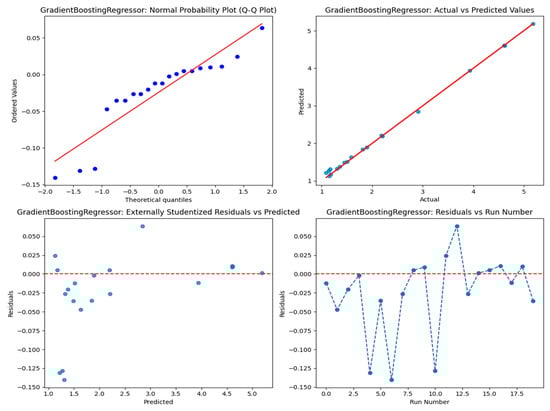
Figure 10. Residuals plots analyzing gradient boosting regression model for tridem axle.

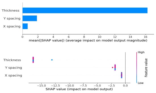
Figure 11. SHAP value analysis for tridem axle model features.

3.3. Discussion

This study analyzes the effectiveness of response surface methodology (RSM) and machine learning techniques in predicting stress levels under various axle configurations, including single, tandem, and tridem axles with dual tires. RSM is proven to be a reliable statistical approach for figuring out correlations between tire spacing, pavement thickness, and stress distribution. The investigation demonstrated that stress levels decrease dramatically with deeper evaluation points, highlighting the significance of depth in pavement design. Additionally, RSM emphasized how reduced tire spacing leads to higher stress levels due to stress overlap, establishing a significant relationship between these variables. Among the RSM models, the quadratic model stood out for its predictive strength, supported by high adjusted R² values and statistically significant p-values.

On the other hand, machine learning models, especially gradient boosting, displayed superior prediction accuracy, obtaining the lowest mean squared error (MSE) and root mean squared error (RMSE) across all axle types. However, SHAP value analysis provides a deeper insight on variable relevance. While RSM emphasized the considerable importance of tire spacing on stress levels, machine learning models suggested a lesser function for spacing, with pavement thickness appearing as the most influential element in stress forecasts. This finding highlights how machine learning excels at uncovering complex relationships between variables and pinpointing other factors that influence stress distribution.

While some machine learning models, like decision tree, showed a tendency to overfit, gradient boosting and random forest consistently produced reliable and accurate results. SHAP analysis also provided valuable insights into the importance of various features, showing that, while tire spacing does have an impact, it is not the main factor driving stress effects. Residuals plots offered further validation for the machine learning models by showing that they satisfied crucial assumptions, such as residual independence and consistency.

In conclusion, RSM gives a structured and methodical approach to predicting stress, while machine learning provides the flexibility and precision needed to capture the dynamic nature of pavement behavior. Through implementing these methodologies, researchers can acquire a deeper understanding of pavement performance. RSM can develop initial hypotheses, and machine learning can enhance these predictions with real-world data. Therefore, this strategy has the potential to customize pavement design, leading to stronger, more durable solutions for a variety of situations while encouraging innovation in engineering techniques.

4. Conclusions

This study aimed to investigate fixed traffic loads, focusing on stress prediction for different axle configurations, including single, tandem, and tridem axles; the conclusions are as follows:

• There is an inverse relationship between the generated stress and the depth of the pavement for single, double, and triple axles. The greater the depth, the lower the stress.
• The spacing between tires in the X and Y directions has a significant effect on the stress. As the spacing decreases, the stress notably increases due to the overlap.
• The use of response surface methodology (RSM) successfully developed models for the generated stress from single, tridem, and triple axles. However, applying a base-10 logarithmic transformation significantly improved the accuracy of the models.
• The quadratic model showed the best performance in predicting stress across all axle configurations. Moreover, it fulfilled all essential statistical assumptions, including normality, homoscedasticity, independence, and linearity, confirming the validity and reliability of the results.
• The analysis of machine learning models showed that gradient boosting showed better performance than the other models in predicting stress.
• Combining RSM and machine learning offers a better understanding of pavement performance. This integrated approach can lead to more effective design strategies, enhancing durability and overall performance.

Future work should focus on multi-layer validation, dynamic loading, and real-world applicability to transition from theoretical models to practical engineering solutions. In particular, future research should investigate both horizontal and vertical stress responses under traffic loads. Collaborations with transportation agencies to acquire field data would add significant value.

References

- Bhandari, S.; Luo, X.; Wang, F. Understanding the effects of structural factors and traffic loading on flexible pavement performance. Int. J. Transp. Sci. Technol. 2023, 12, 258–272. [Google Scholar] [CrossRef]
- Adlinge, S.S.; Gupta, A.K. Pavement deterioration and its causes. Int. J. Innov. Res. Dev. 2013, 2, 437–450. [Google Scholar]
- Zeiada, W.A.; Underwood, B.S.; Kaloush, K.E. Impact of asphalt concrete fatigue endurance limit definition on pavement performance prediction. Int. J. Pavement Eng. 2017, 18, 945–956. [Google Scholar] [CrossRef]
- Canestrari, F.; Ingrassia, L.P. A review of top-down cracking in asphalt pavements: Causes, models, experimental tools and future challenges. J. Traffic Transp. Eng. (Engl. Ed.) 2020, 7, 541–572. [Google Scholar] [CrossRef]
- Alencar, G.; de Jesus, A.M.; Calçada, R.A.; da Silva, J.G.S. Fatigue life evaluation of a composite steel-concrete roadway bridge through the hot-spot stress method considering progressive pavement deterioration. Eng. Struct. 2018, 166, 46–61. [Google Scholar] [CrossRef]
- Di Mascio, P.; Moretti, L.; Capannolo, A. Concrete block pavements in urban and local roads: Analysis of stress-strain condition and proposal for a catalogue. J. Traffic Transp. Eng. 2019, 6, 557–566. [Google Scholar] [CrossRef]
- Zeng, Z.; Underwood, B.S.; Kim, Y.R. A state-of-the-art review of asphalt mixture fracture models to address pavement reflective cracking. Constr. Build. Mater. 2024, 443, 137674. [Google Scholar] [CrossRef]
- Al-Janabi, A.J.; Obaid, H.A. Analysis of the Impact of Overloading for Trucks on the Design Life of Flexible Pavement. In IOP Conference Series: Earth and Environmental Science; IOP Publishing: Bristol, UK, 2024; Volume 1374, p. 012089. [Google Scholar]
- Papagiannakis, A.T.; Masad, E.A. Pavement Design and Materials; John Wiley & Sons: Hoboken, NJ, USA, 2024. [Google Scholar]
- Huang, Y.H. Pavement Analysis and Design; Pearson Prentice Hall: Upper Saddle River, NJ, USA, 2004. [Google Scholar]
- Sun, J.; Oh, E.; Chai, G.; Ma, Z.; Ong, D.E.; Bell, P. A systematic review of structural design methods and nondestructive tests for airport pavements. Constr. Build. Mater. 2024, 411, 134543. [Google Scholar] [CrossRef]
- Mahajan, G.R.; Radhika, B.; Biligiri, K.P. A critical review of vehicle-pavement interaction mechanism in evaluating flexible pavement performance characteristics. Road Mater. Pavement Des. 2022, 23, 735–769. [Google Scholar] [CrossRef]
- Clary, L. An examination of the affect of axle spacing on the deformation of thin membrane pavements. In Masters Abstracts International; Library and Archives Canada = Bibliothèque et Archives Canada: Ottawa, ON, Canada, 2010; Volume 48. [Google Scholar]
- Singh, A.K.; Sahoo, J.P. Analysis and design of two layered flexible pavement systems: A new mechanistic approach. Comput. Geotech. 2020, 117, 103238. [Google Scholar] [CrossRef]
- Huang, Y.H. Computation of equivalent single-wheel loads using layered theory. In Highway Research Record 291; Highway Research Board: Washington, DC, USA, 1969; pp. 144–155. [Google Scholar]
- Zakaria, N.M.; Yusoff, N.I.M.; Hardwiyono, S.; Mohd Nayan, K.A.; El-Shafie, A. Measurements of the stiffness and thickness of the pavement asphalt layer using the enhanced resonance search method. Sci. World J. 2014, 2014, 594797. [Google Scholar] [CrossRef] [PubMed]
- Ojha, K.N. Flexible Pavement Thickness (A Comparative Study Between Standard and Overloading Condition). Am. Sci. Res. J. Eng. Technol. Sci. (ASRJETS) 2019, 58, 159–181. [Google Scholar]
- Harrell, F.E., Jr.; Harrell, F.E. General aspects of fitting regression models. In Regression Modeling Strategies: With Applications to Linear Models, Logistic and Ordinal Regression, and Survival Analysis; Springer: Cham, Swizterland, 2015; pp. 13–44. [Google Scholar]
- Alnadish, A.; Aman, Y. Mechanistic approach for reducing the thickness of asphalt layer incorporating steel slag aggregate. Civ. Eng. J. 2018, 4, 334–345. [Google Scholar] [CrossRef]
- Wilches, F.J.; Caballero Guerrero, Á.R.; Patrón Lambraño, G. Modeling of Asphalt Pavement Considering the Application of Empirical and Mechanistic Design Methodologies. Int. J. Eng. Res. Technol. 2020, 13, 3919. [Google Scholar] [CrossRef]
- Fuentes, L.; Taborda, K.; Hu, X.; Horak, E.; Bai, T.; Walubita, L.F. A probabilistic approach to detect structural problems in flexible pavement sections at network level assessment. Int. J. Pavement Eng. 2022, 23, 1867–1880. [Google Scholar] [CrossRef]
- Bueno, B.A.V.; Arenas, M.J.P.; Lugo, A.E.A.; Jaimes, V.E.M.; Ariza, C.A.F.; Chio, G. Deep neural networks for sensitivity assessment of design variables on the structural design parameters of flexible pavements for low-traffic volume roads. Rev. Colomb. Tecnol. Av. (RCTA) 2023, 2, 122–130. [Google Scholar]
- López, R.; Fernández, C.; Pereira, F.J.; Díez, A.; Cara, J.; Martínez, O.; Sánchez, M.E. A comparison between several response surface methodology designs and a neural network model to optimise the oxidation conditions of a lignocellulosic blend. Biomolecules 2020, 10, 787. [Google Scholar] [CrossRef]
- Omranian, S.R. Application of response surface method for analyzing pavement performance. In Response Surface Methodology in Engineering Science; Kayaroganam, P., Ed.; IntechOpen: London, UK, 2021; pp. 1–13. [Google Scholar]
- Montgomery, D.C. Design and Analysis of Experiments; John Wiley & Sons: Hoboken, NJ, USA, 2017. [Google Scholar]
- Veza, I.; Spraggon, M.; Fattah, I.R.; Idris, M. Response surface methodology (RSM) for optimizing engine performance and emissions fueled with biofuel: Review of RSM for sustainability energy transition. Results Eng. 2023, 18, 101213. [Google Scholar] [CrossRef]
- Justo-Silva, R.; Ferreira, A.; Flintsch, G. Review on machine learning techniques for developing pavement performance prediction models. Sustainability 2021, 13, 5248. [Google Scholar] [CrossRef]
- Tamagusko, T.; Ferreira, A. Machine Learning for Prediction of the International Roughness Index on Flexible Pavements: A Review, Challenges, and Future Directions. Infrastructures 2023, 8, 170. [Google Scholar] [CrossRef]
- Alnadish, A.M.; Aman, M.Y.; Katman, H.Y.B.; Ibrahim, M.R. Characteristics of warm mix asphalt incorporating coarse steel slag aggregates. Appl. Sci. 2021, 11, 3708. [Google Scholar] [CrossRef]
- Rosopa, P.J.; Schaffer, M.M.; Schroeder, A.N. Managing heteroscedasticity in general linear models. Psychol. Methods 2013, 18, 335. [Google Scholar] [CrossRef]
- Schmidt, A.F.; Finan, C. Linear regression and the normality assumption. J. Clin. Epidemiol. 2018, 98, 146–151. [Google Scholar] [CrossRef]
- James, G.; Witten, D.; Hastie, T.; Tibshirani, R.; Taylor, J. Linear regression. In An Introduction to Statistical Learning: With Applications in Python; Springer International Publishing: Cham, Switzerland, 2023; pp. 69–134. [Google Scholar]
Disclaimer/Publisher’s Note: The statements, opinions and data contained in all publications are solely those of the individual author(s) and contributor(s) and not of MDPI and/or the editor(s). MDPI and/or the editor(s) disclaim responsibility for any injury to people or property resulting from any ideas, methods, instructions or products referred to in the content. |
© 2025 by the authors. Licensee MDPI, Basel, Switzerland. This article is an open access article distributed under the terms and conditions of the Creative Commons Attribution (CC BY) license (https://creativecommons.org/licenses/by/4.0/).