An Enhanced Contrastive Ensemble Learning Method for Anomaly Sound Detection

Abstract

This paper proposes an enhanced contrastive ensemble learning method for anomaly sound detection. The proposed method achieves approximately 6% in the AUC metric in some categories and achieves state-of-the-art performance among self-supervised models on multiple benchmark datasets. The proposed method is effective in automatically monitoring the operating conditions of the production equipment by detecting the sounds emitted by the machine, to provide an early warning of potential production accidents. This method can significantly reduce industrial monitoring costs and increase monitoring efficiency to improve manufacturing facility productivity effectively. Existing detection methods face challenges with data imbalance caused by the scarcity of anomalous samples, leading to performance degradation. This paper proposes an enhanced data augmentation method that improves model robustness by allowing the data to retain the original features while adding noise close to the real environment through a simple operation. Secondly, model feature extraction is enhanced by using channel attention to fuse time-frequency features. Thirdly, this paper proposes a simple anomaly sample generation method, which can automatically generate real pseudo anomaly samples to help the model gain anomaly detection capability and reduce the impact of data imbalance. Finally, this paper proposes a statistical-based bias compensation that further mitigates the impact of data imbalance by distributing samples through statistical induction. Experimental verification confirms that these changes enhance anomalous sound detection capability.

1. Introduction

Anomaly sound detection (ASD) is an algorithm used to ascertain whether the sound emitted by an object under test is in an abnormal state. This algorithm is widely applied in various fields, particularly in the industrial manufacturing systems [1,2]. Machine equipment generates sounds during operation, which reflect its current working status. Utilizing ASD algorithms can effectively monitor the operational conditions of the machines being tested and issue early warnings for potential anomalies, thereby preemptively averting potential production accidents and machine failures. However, in reality, it is often challenging to obtain a large number of valid anomaly sound samples. Consequently, anomaly sound detection tasks frequently encounter the issue of extreme data imbalance. This imbalance also leads to a blurred definition boundary between normal and anomaly samples, which will affect the accuracy of anomaly sound detection methods.

ASD generally requires sufficient positive and negative samples. However, in the real-world scenarios, collecting comprehensive and representative negative samples can be challenging due to their inherent diversity and scarcity. Consequently, many existing studies exploit only positive samples instead [3,4]. One of the most common methods is based on statistics, such as the outlier detection [5], K-means [6] and density-based detection method [7]. This method assesses whether the input sample is anomalous by measuring the distance from the observation to the centroid of each sample cluster. In recent decades, classifier-based methods have become a trend. For example, deep learning-based methods [8,9] train a neural network to find the relationships between the sound representations and the equipment status. A classifier is then used to detect anomalies. What is more, reconstruction-based methods can also be applied to anomaly detection, such as autoencoder [10] and Generative Adversarial Networks (GANs) [11]. This method performs anomaly detection by calculating the reconstruction error between the reconstructed sample and the input sample. After training, the model can only accurately reconstruct and map normal samples. Therefore, abnormal samples often cannot be reconstructed properly, resulting in a larger reconstruction error.

Although these methods are effective, they still have many drawbacks. For example, statistical-based methods directly adopt feature reduction techniques, which may fail to accurately capture the distribution of complex real-life data. This can lead to excessively large clusters, thereby compromising the anomaly detection capability. Similarly, reconstruction-based methods are also struggle with complex and high-dimensional data, making it difficult to efficiently distinguish between normal and abnormal samples when determining the decision boundary, which affects the model’s judgment results. While GANs can mitigate this shortcoming, most GAN models have strict requirements for training samples, and the performance of the generator and discriminator affect each other. These issues also contribute to poor model performance. With the development of deep learning networks, using complex neural network models can effectively fit high-dimensional data to obtain a more accurate feature distribution. However, in reality, it is often difficult to collect a large and diverse set of abnormal samples. This results in complex neural network models performing anomaly detection in the absence of abnormal samples, leading to a significant reduction in model performance as the model is unable to understand the distribution of abnormal samples and potentially causing overfitting. Additionally, due to data imbalance, the model may develop bias, leading to degraded detection performance or even model collapse, resulting in trivial solutions. Although numerous methods [12,13] exist to address the bias problem in neural networks caused by data imbalance, most of these methods are based on federated learning. Therefore, when applied in real manufacturing environments, they are constantly faced with communication and device heterogeneity issues, while these methods may be difficult to apply in large-scale industrial deployment environments.

Therefore, this paper proposes a novel self-supervised learning approach. The proposed network is not only able to learn the feature representations of normal samples while mitigating the bias arising from the imbalanced dataset, but it is also able to swiftly generate effective abnormal samples and attend to learn the feature distribution of the potentially real-life abnormal samples. The detailed contributions are as follows. Firstly, this paper employs a novel improved spectrogram augmentation method and proposes a cross-domain data representation approach specifically for original audio format data, encompassing features in the time domain, frequency domain and statistical domain. Secondly, this paper proposes an improved novel self-supervised learning network for anomaly sound detection tasks. After being tested on multiple datasets, the model demonstrates excellent performance. Lastly, this paper proposes a simple method for generating anomaly samples, which can effectively assist the model in learning the features of potential real-life anomaly samples.

2. Materials and Methods

2.1. Motivation

As neural networks continue to evolve, neural network-based deep learning methods have increasingly become the primary approach for ASD. However, in real-life industrial manufacturing environments, it is difficult to obtain accurate data labels, making it difficult for common deep learning approaches to perform. This results in the formulation of a solution based on a self-supervised approach. The self-supervised learning process enables the model to effectively capture the global feature distribution. Self-supervised learning methods spontaneously mine feature information based on auxiliary tasks through the construction of these tasks, and generalize this to general features, thereby accomplishing the modeling of the model’s global feature distribution. In the task of ASD, common self-supervised learning approaches employ auxiliary classification methods or contrastive learning techniques. For example, reference [14] collects phase and amplitude features from the data, utilizing a self-supervised classification network and attention method for auxiliary classification, thereby enabling the model to acquire feature modeling of normal sample data and realize the capability of abnormal sound detection; reference [15] employs a flow-based density estimation model, integrating self-supervised classification methods with unsupervised density likelihood estimation approaches to enhance the model’s capability for ASD; reference [16] employs contrastive learning method by calculating the cosine angle between positive and negative samples, enabling the model to simultaneously learn the distributions of normal and abnormal features.

Although these techniques may prove effective in the detection of anomalies, the resulting precision may be compromised. This is because the issue of neural network bias, which is caused by the imbalance in the amount of data, is not taken into account in the feature representation. Furthermore, the problem of model collapse, which occurs in the absence of valid anomaly samples, is also overlooked. Consequently, this paper presents a novel model that addresses these issues. It is capable of gathering more comprehensive feature data, rectifying the bias issue inherent to neural networks, and performing multi-domain fusion and adaptive weighting of multi-domain information. Furthermore, it can quickly and effectively generate high-quality anomaly samples during the training process, thereby enhancing the model’s overall anomaly detection capabilities. The model has been subjected to extensive experimentation with multiple datasets, and a comparative analysis of the experimental results has demonstrated its efficacy in anomaly detection and generalization.

2.2. Data Processing

To enhance the performance of the model in capturing the features of the original data, this paper implements multi-domain data processing in the source audio data, encompassing not only the time domain but also the frequency domain and statistical domain. This enables the model to obtain a more comprehensive representation of the data in low dimensions, facilitating a more nuanced and comprehensive understanding of the data. In this paper, the log-mel transform [17] is employed for frequency domain feature analysis and extracts the log-mel power spectrogram and the log-mel magnitude spectrogram from the input audio signals. In contrast, the Mel spectrogram is used to represent the features of the statistical domain.

2.3. Data Augmentation

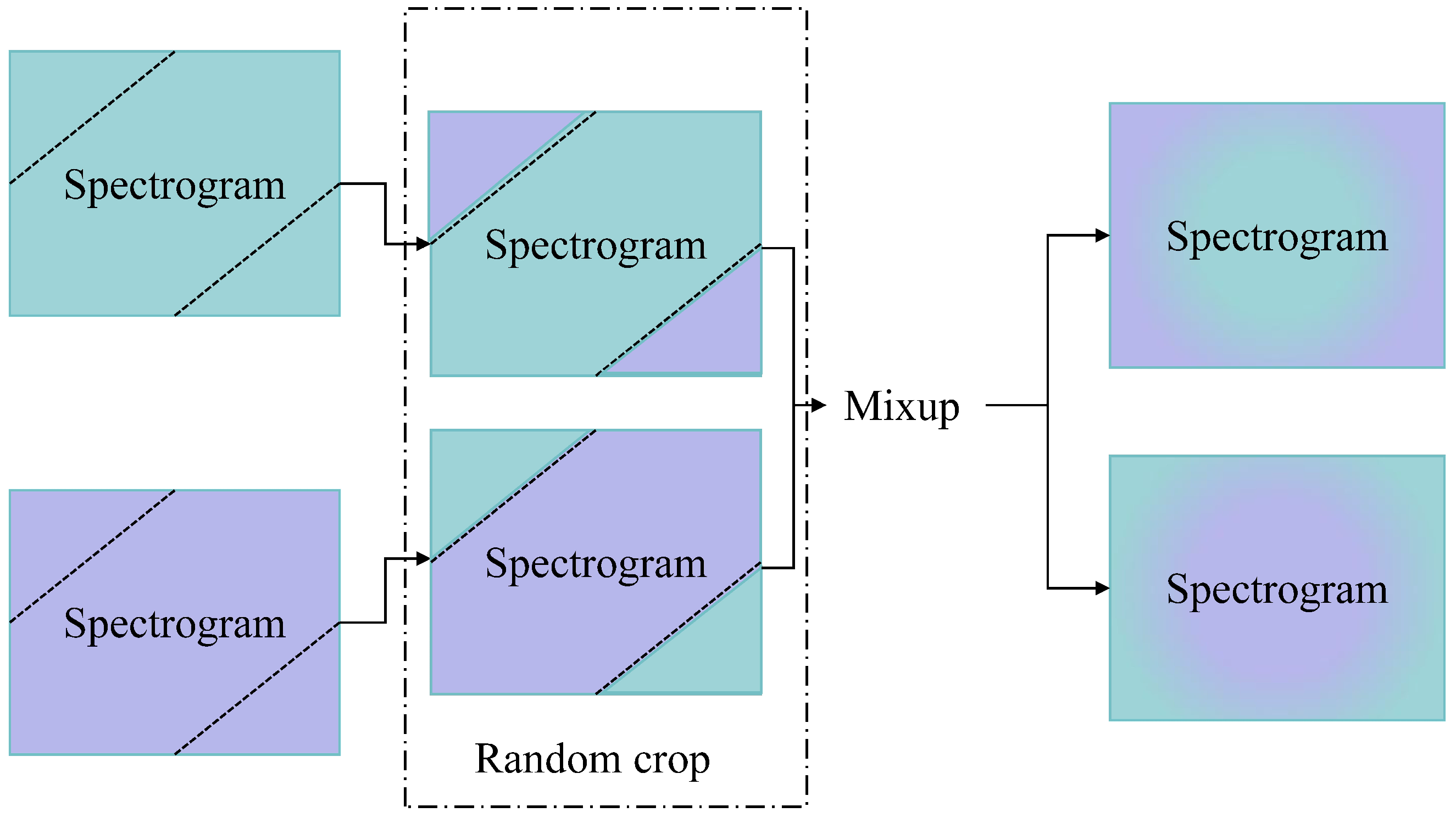
In order to improve the model’s generalization ability, this paper used a mixup [18] based on the audio clipping augmentation approach. For the spectral feature maps, the target spectrograms were randomly cropped at the top left and bottom right, and the clipped portion was spliced with other spectrograms, while mixup enhancement was used to increase the diversity of the data and reduce model overfitting. The procedure is shown in Figure 1. Compared to other cropping augmentation approaches such as cutout [19], the method proposed in this paper ensures the possession of both original and interference features at every time pin and every frequency value. In order to maximize the introduction of interference factors without significantly disturbing the original feature information, the cutting points on the frequency domain axis and the time domain axis are designed to be complementary during the shearing process. The methodology is as follows:

$$\begin{array}{cc}\hfill x& \in (1,{\displaystyle \frac{3}{4}}F),\hfill \\ \hfill y& \in (1,{\displaystyle \frac{3}{4}}T),\hfill \end{array}$$

(1)

where F represents the frequency domain axis length, T represents the time domain axis length, x and y represent the random cropping points on their respective axes, respectively.

Subsequently, a mixup-based augmentation was conducted on the two cropped spectrograms, utilizing a mixing ratio factor to combine the two inputs and the corresponding labels in a specified ratio. The mixup-based augmentation is as follows:

$$\begin{array}{cc}\hfill x& =(1-\lambda )x_1+\lambda x_2,\hfill \\ \hfill y& =(1-\lambda )y_1+\lambda y_2,\hfill \end{array}$$

(2)

where $x_1$, $x_2$ refers to input samples and $y_1$, $y_2$ refers to their corresponding labels. x, y refer to the mixed sample and its label.

2.4. Contrastive-Based Spectrogram Domain Model

For the raw data, this paper transforms the signal data into log-mel power spectrogram and log-mel energy spectrogram via log-mel transformation [17], and then concatenates these two spectrograms via channel dimension, which enhances information features of frequency domain at minimal cost.

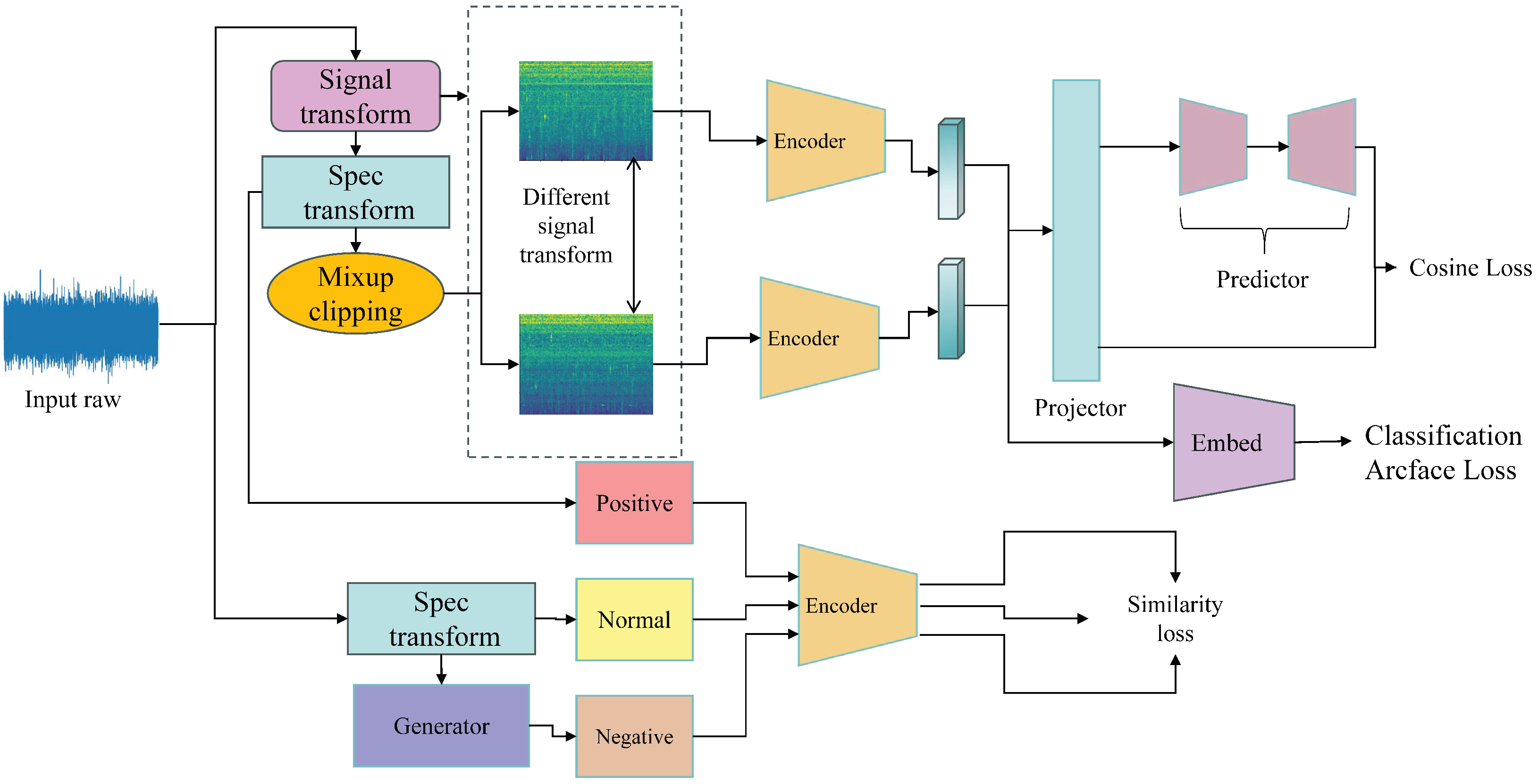
After that, this paper designs an improved contrastive learning-based model. The structure is depicted in Figure 2. This model is divided into a pre-training feature contrastive training and anomalous samples fine-tuning model. The aim of the pre-training process is to allow the model to gain feature extraction capability for each category of sound frequency domain data by increasing the similarity of two samples of the same category. The purpose of the fine-tuning process is to generate anomaly samples through the anomaly sample generator to give the model anomaly detection capability and to improve the fit of the anomaly decision boundary.

2.4.1. Pre-Train Progress

During the pre-training progress, a multi-task learning approach is used to improve model performance and help the model to converge. The pre-training structure is improved from the Simple Siamese network (Simsiam) [20]. This paper not only calculates the cosine similarity, but also employs a self-supervised classification task to further enhance the model feature representation capabilities. This paper employs GhostnetV2 [21] model as the feature embedding network which can not only accurately capture features but also reduce the number of model parameters, thereby enhancing computational speed. For this backbone network, this paper only uses the front feature extraction convolutional layer without using the last fully connected classification layer. Moreover, to further improve the model generalization ability and data diversity, this paper randomly employs signal transformations such as time shift, pitch shift, fade in/out and add noise. The time shift transformation shifts the audio signal either forward or backward. In this paper, the time shift rate is chosen from the range of 0–56. The pitch shift transformation shifts the pitch of the waveform. In this paper, the step to shift the waveform is set to −20. The fade in/out transformation adds a fade in or fade out to a waveform at its beginning or end. This paper uses two types of fading: exponential and half sinusoidal. And adding noise transformation inserts a white Gaussian noise in the waveform. In this paper, the signal-to-noise ratio (SNR) is chosen in the range of [−10, 10]. After applying these transformations, the input spectrogram maps are then fed into the Simsiam structure. By maximizing the similarity of the same class samples, the backbone model can efficiently model sample features. Moreover, in order to improve the model performance better, this paper designs a self-supervised classification task for this backbone model.

For the contrastive learning pre-trained model, the total cosine similarity can be calculated as follows:

$$\begin{array}{c}\hfill L={\displaystyle \frac{1}{2}}D(p_1,z_2)+{\displaystyle \frac{1}{2}}D(p_2,z_1),\\ \hfill D(d_1,d_2)=-{\displaystyle \frac{d_1}{\parallel d_1{\parallel }_2}}·{\displaystyle \frac{d_2}{\parallel d_2{\parallel }_2}},\end{array}$$

(3)

where p and z represent two feature vectors, and D represents the cosine similarity function. However, due to the lack of different class samples, the model will collapse easily during the training progress. Therefore, to avoid this problem, a stop-gradient operation [20] is imposed on one of the feature vectors. So the final cosine similarity loss functions is reformulated as follows:

$$\begin{array}{c}\hfill L={\displaystyle \frac{1}{2}}D(p_1,stopgrad\left(z_2\right))+{\displaystyle \frac{1}{2}}D(p_2,stopgrad\left(z_1\right)),\end{array}$$

(4)

After the contrastive learning progress, the backbone is trained with an auxiliary classification task. In the auxiliary classification task, the feature vectors of the input spectrograms from the Siamese network are fed into the embedding head, which outputs the predicted label values. Subsequently, the ArcFace [22] loss function is utilized to calculate the loss. The arcrface loss functions is as follows:

$$L=-{\displaystyle \frac{1}{N}}\sum _{i=1}^{N}log{\displaystyle \frac{e^{s\left(cos({\theta }_{y_i}+m)\right)}}{e^{s\left(cos({\theta }_{y_i}+m)\right)}+{\sum }_{k=1,k\ne y_i}^K{e}^{scos{\theta }_k}}},$$

(5)

where N represents the batch size number, s represents the scale parameter, m represents the margin parameter, ${\theta }_{y_i}$ represents the angle value of the target category corresponding to the sample $y_i$, ${\theta }_k$ represents the angle value of the non-target category corresponding to sample $y_i$ and K represents the number of non-target categories.

2.4.2. Fine-Tune Progress

After pre-training, the backbone model is immediately fine-tuned. This paper employs a simple novel negative generator which can generate pseudo-negative samples from normal samples. This paper uses two simple methods to generate fake samples. The first is Spectrogram Flip (SF) and the second is Spectrogram Plus (SP). The pseudo-anomaly sample example is shown in Figure 3.

SF: This paper inverted the top and bottom for the input spectrogram. This operation allows the normal information highlighted in the normal sample to be overwritten. For example, in such cases wherein the regular data are a high-frequency sound, the corresponding anomalous data may be a low-frequency sound. Flipping can then be applied to generate negative samples that are similar to the real negative samples. This is achieved by shifting the energy from the high-frequency portion of the sample to the low-frequency portion. As a result, the low-frequency portion becomes more prominent than the high-frequency portion, and the energy of the high-frequency portion is displaced by the energy of the low-frequency portion. As a result, the flipped sample can be considered as a real negative sample.

SP: This paper performed a stacking operation for the input spectrogram. Within the spectrograms, the normal features of the sound is often prominent, while the environmental noise features are relatively inconspicuous. During the stacking process, the original sound features may exceed their original normal range due to multiple stacking, leading to over-noise anomalies and the formation of noise. Furthermore, after stacking, some of the originally weak noise features may replace the original sound features, causing the model’s focus to shift from normal features to environmental noise features.

After generating pseudo samples, in order to help the model achieve precise anomaly detection boundaries while improving its generalization capability, this paper establishes three sample clusters. Among them, the original samples are designated as the main anchor cluster, the samples generated by the generator form the anomaly cluster and the samples enhanced through signal augmentation constitute the generalization cluster. After generating three different categories of clusters, this paper then employs an improved similarity loss function to train the encoder backbone. The improved loss function takes into account both cosine angle and Euclidean distance, and this loss function can adequately generalize the separation of vector angles and spatial distances between clusters with different attributes which can improve the model performance. The improved loss function is as follows:

$$\begin{array}{cc}\hfill L_{cos}& =-D(x_{anchor},x_{pos})+D(x_{anchor},x_{neg}),\hfill \\ \hfill L_{dis}& ={\parallel x_{anchor}-x_{pos}{\parallel }_2}^2-{\parallel x_{anchor}-x_{neg}{\parallel }_2}^2+m,\hfill \\ \hfill L_{loss}& ={\displaystyle \frac{1}{N}}\sum _1^N(L_{dis}+\alpha ){exp}^{(s{L}_{cos}+\beta )},\hfill \end{array}$$

(6)

where $\alpha$, $\beta$ and s are three scale parameters, m represents a distance margin, $x_{anchor}$ represents the original anchor sample, $x_{pos}$ represents the augmented positive sample against the anchor sample and $x_{neg}$ represents the negative anomaly sample against the anchor sample. In this paper, m is set to 0.05, s is set to 1, $\alpha$ is set to 0.01 and $\beta$ is set to 0.005.

2.5. Time Domain Model

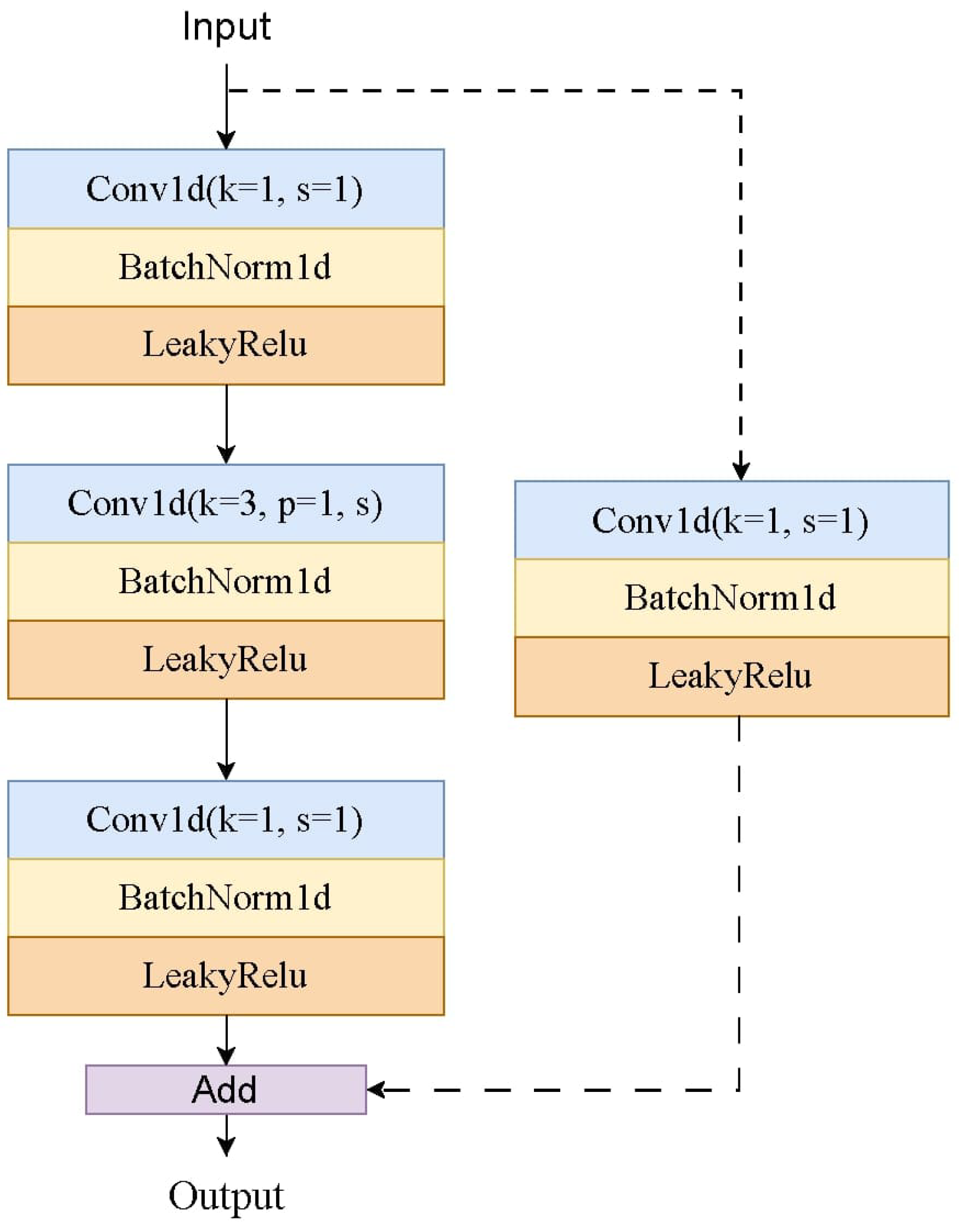
Although spectrogram-based networks are capable of effectively extracting features, due to the nature of convolution calculations, spectral-based network models tend to capture only frequency domain features while neglecting the causality and correlation of time domain features. In order to fully represent the features of the input data, this paper used not only the frequency features, but also the time domain features. This paper designs a time domain CNN model, the model framework of which is summarized in

Table 1. Temporal model structure: The block contains three convolutional blocks which form an inverted residue module. In each block, t represents intermediate dimension scale factor of the inverted residual module of the block, c represents output dimension of each layer and s stands for the stride size of each layer.

Input	Operator	Parameters
		t	c	s
1 × 160,000	Conv1d (k = 256)	-	16	64
1 × 1250	block	3	32	1
1 × 1250	block	3	32	2
1 × 625	block	3	32	2
1 × 313	block	2	64	3
1 × 105	block	2	128	2
1 × 53	block	2	256	1
1 × 53	block	2	256	2
1 × 27	block	2	256	2
1 × 14	block	2	256	2
1 × 7	block	2	256	1
1 × 7	Avgpool (k = 7)	-	512	1

. In this model, the first convolutional layer takes a convolutional kernel of size 256. The reason for using a large convolutional kernel is to take into account the fact that the sampling frequency of the input samples is 16KHz, so a small kernel size will not only affect the response speed of the model, but also reduce the global feature extraction ability of the shallow network. The model then utilizes multiple blocks for subsequent feature extraction. The structure of the block is shown in Figure 4. In each block, all the layers employ depthwise separable convolutions, which can ensure feature extraction capabilities while simultaneously reducing computational load and enhancing computational speed.

2.6. Domain Fusion Model

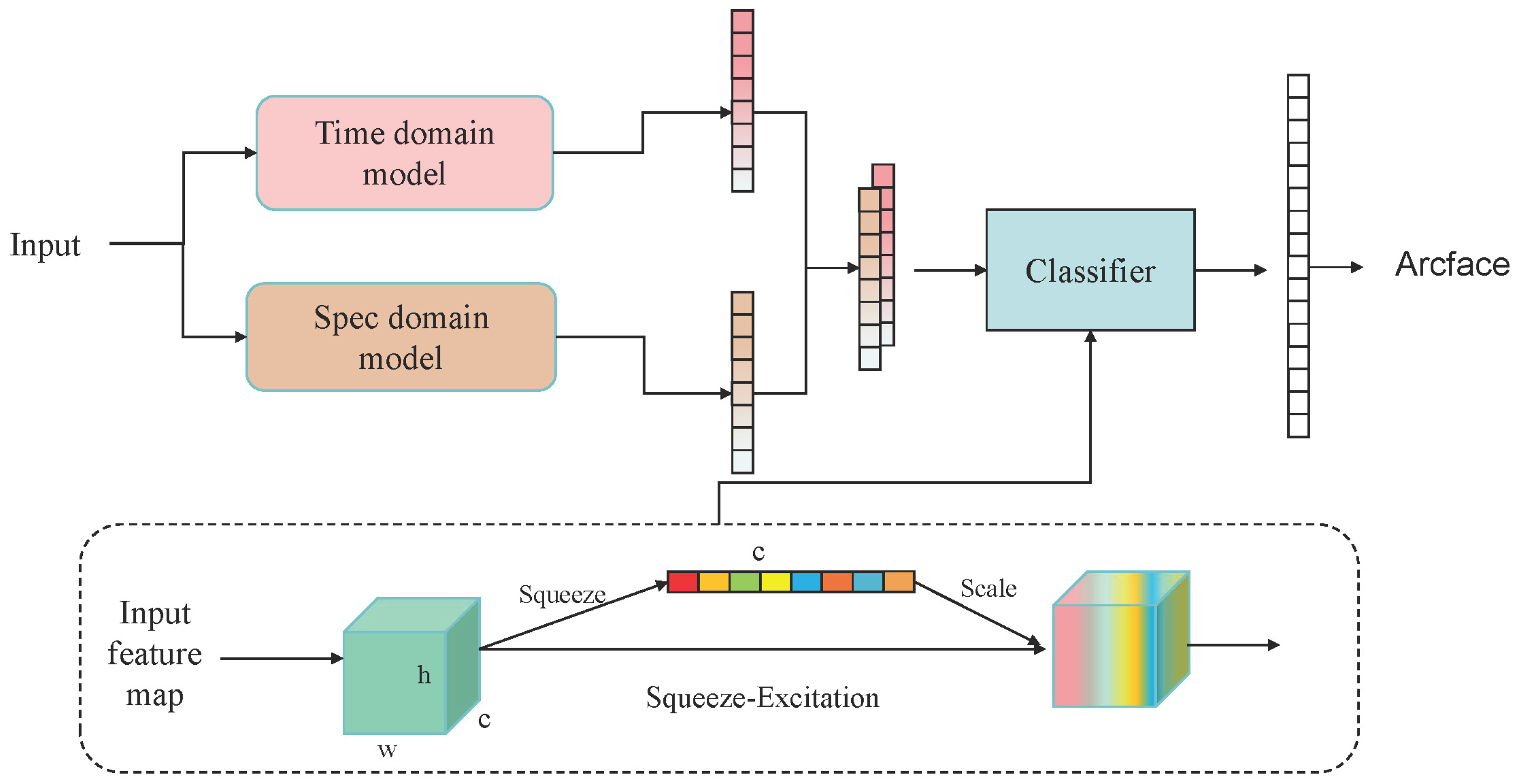
In order to be able to unite the time-frequency domain features, this paper ensembles the feature extraction backbone networks from the frequency domain and time domain models. The fusion method is illustrated in Figure 5. The fusion model first concatenates the feature vectors from both time and frequency domains along the channel dimension. Subsequently, the concatenated feature vector is fed into a classifier. This classifier employs multiple Squeeze-and-Excitation Blocks (SEBlock) [23] to perform channel-wise adaptive weighting on the input features. Finally, for the classification prediction output, the ArcFace function is used to calculate the loss value for model convergence. During the training process, neither the time domain model nor the frequency domain model participates in gradient updates; only the classifier participates in the back-propagation process. The aim is to ensure that the feature representation capabilities of the two models remain unchanged, thereby guaranteeing optimal feature modeling capability. In this paper, the channel attention-based fusion method is employed instead of directly utilizing time-frequency features. This is because the direct utilization of time-frequency domain features may not be able to specifically represent the feature distribution of the input samples. By using the channel attention mechanism, the model can automatically extract the correlation between each feature channel and automatically weight the channels according to the degree of importance, which can help the model focus on feature maps that are more critical to the target task than directly extracting features from the time-frequency domain, thus improving the model performance. The overall fusion classifier structure is shown in

Table 2. The fusion classifier structure: FC represents the fully connected layer, layer represents the convolutional layer and SEBlock represents the channel attention block. The batchnorm is used in each convolutional layer, and the PRELU activation function is used in the first two convolutional layers. In each SEBlock, the mid-channel factor is set to 0.5.

Layer	In Channel	Out Channel	Kernel Size
layer1	2	16	1
SEBlock	16	16	1
layer2	16	64	3
SEBlock	64	64	1
layer3	64	256	3
layer4	256	512	6
layer5	512	128	1
FC	128	16	-

.

2.7. Statistics Domain Model

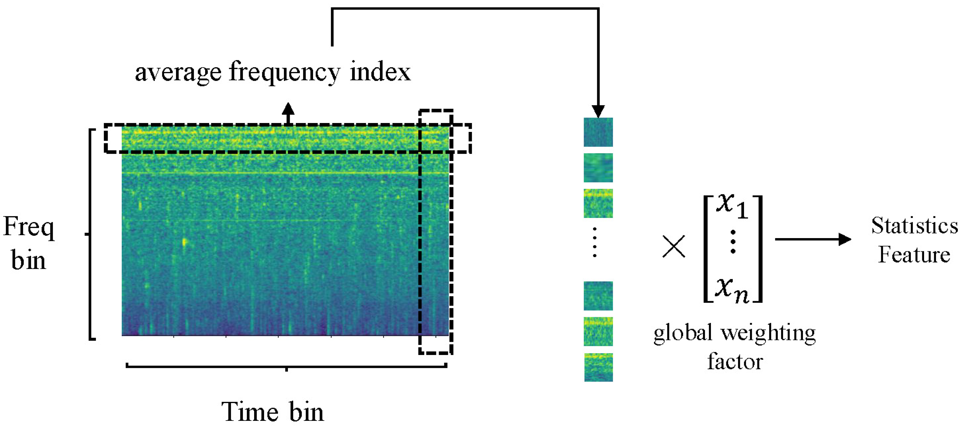
In most anomaly detection tasks, models often encounter the issue of severe data imbalance. Even with the introduction of generators, it remains difficult to mitigate the model bias caused by the imbalance in the original data, which subsequently degrades the model’s performance. Therefore, to address this issue, this paper proposes a method of using statistically weighted average frequency-domain features to correct feature bias. For the spectrogram of the input data, this paper calculates the global average value of each frequency along the time axis. Finally, a global weighting is applied based on the magnitude of each frequency’s average value, meaning that frequencies with larger average values will receive greater weights, while those with smaller average values will receive smaller weights. Compared to statistical feature representation methods based on extreme values, the method used in this paper not only reflects the average performance of each frequency across the entire time axis but also highlights the importance of different frequencies based on their weighted weights. The average frequency index can be calculated using the following formula:

$$\begin{array}{c}\hfill y_i={\displaystyle \frac{1}{N}}\sum _{j=1}^N{x}_j,\end{array}$$

(7)

where N represents the batch size number, i represents the frequency bin and $x_j$ represents each sample bin. The global weighting factors are calculated as follows:

$$\begin{array}{c}\hfill {\lambda }_i={\displaystyle \frac{y_i}{{\sum }_{f=1}^M{y}_f}},i\in (1,M),\end{array}$$

(8)

where i represents the frequency bin, M represents the total frequency bin numbers and $y_i$ represents the average frequency index of the current current frequency. The full process is shown in Figure 6.

2.8. Ensemble Evaluator Model

This paper employs an ensemble approach for anomaly assessment on the input data. The anomaly scores are obtained through a Gaussian Mixture Model (GMM), which combines multiple Gaussian distributions. By adjusting the parameters of the GMM, the model can approximate almost any data distribution. After evaluating both the statistical domain model and the time-frequency domain fusion mode, an ensemble method is utilized to obtain the final evaluation score. The calculation method is described as follows:

$$\begin{array}{c}\hfill Score=\sum _{i=1}^2{\lambda }_{i}GM{M}_i,\end{array}$$

(9)

where $\lambda$ is weight parameter and i represents the i-th model. In this paper, the weight for the fusion model is set to 0.9, with the aim of fulling leveraging the discriminative performance of the model. For the statistical domain model, the weight is assigned as 0.1. This is because the role of the statistical model is merely to introduce statistical features and reduce the bias caused by data imbalance. Therefore, only a partial detection capability of this model is needed. Although this paper applies fixed discriminant weights to the two models, several tests indicate that better model performance can be achieved by adjusting the weights according to the characteristics of different test objects. However, since the interference noise in the original data is not adequately considered when using statistical factors, if the statistical model assigns a larger weight to some categories of data, it will instead reduce the model’s detection ability.

3. Results

3.1. Dataset

To fully test the capability of the proposed model, the MIMII dataset [24], DCASE2020 task2 dataset and MIMII DUE dataset [25] are used for validation experiments. In ASD tasks, the primary official evaluation metric is the Area Under the Curve (AUC) value, which reflects the area under the ROC curve. In the MIMII dataset and the DCASE2020 task2 dataset, the primary focus of testing was the model’s ability to detect anomalies without training on anomalous samples. In the MIMII DUE dataset, the main objective was to evaluate the model’s capability for transfer anomaly sound detection without applying domain adaptation, thereby assessing the model’s robustness and generalization ability. In the MIMII dataset, there are only four different categories. In the DCASE2020 task2 dataset, it contains the MIMII dataset and Toyadmos dataset, with six different categories. In the MIMII DUE dataset, it contains five different categories. Within each category, the normal data for the source domain and a small amount of data for the target domain are included.

In these datasets, the machine objects included are common types of machines found in industrial environments, such as slide rails, pumps, fans and so on. In the training set, only normal samples are included. In each training sample, the sound data are captured in a realistic manufacturing environment, which means that each audio datum contains not only the primary feature data of the machine being evaluated but also numerous disturbing noises from the surrounding environment, including the disruptive sounds of other industrial machines and parts of human voices. In the test set, the data consist of normal and abnormal sound samples, which are also derived from the real manufacturing system environment and covers a number of different types of anomalies in order to simulate the manufacturing environment under real-life conditions. In addition to this, in some test sets, to further satisfy the reality of the manufacturing environment, the test data also include the sound of the manufacturing machine under different production conditions, such as different temperatures, humidity and weather. Therefore, by considering these characteristics, these benchmark datasets are selected in this paper to validate the performance of the proposed model.

3.2. Implementation

During the data mixup augmentation, the mixing ratio factor is set to 0.4. In the process of spectrogram transformation, the number of Mel filters is set to 224, the hop length is set to 512 and the number of FFT points is set to 2048.

For the frequency domain network model, during the pre-training stage, the number of training epochs is 50, with a batch size of 128. The backbone network employs the SGD optimizer, with an initial learning rate of 0.05, a weight decay factor of 0.005 and a momentum factor of 0.9. The auxiliary network uses the AdamW optimizer [26] with an initial learning rate of 0.01. Additionally, to ensure good convergence stability, this paper applies cosine decay specifically for this network. During the fine-tuning comparison stage, the AdamW optimizer is used with an initial learning rate of 0.001, a weight decay factor of 0.0005, a batch size of 64 and a number of training epochs of 50.

For the time domain network model, the AdamW optimizer is used with an initial learning rate of 0.005, a weight decay factor of 0.0005, a batch size of 128 and a number of training epochs of 200.

For the time-frequency domain hybrid model, the SGD optimizer is used with a learning rate of 0.05, a weight decay factor of 0.005, a momentum factor of 0.9, a batch size of 128 and a number of training epochs of 20.

For the two GMM estimators, the number of mixing components is set to 1 and the number of EM iterations is set to 1000.

3.3. Experiment Results

The AUC test results for the model are presented in

Table 3. AUC scores in three datasets: Since most open-source papers and code evaluation metrics only provide the AUC value, the AUC is primarily used as the main indicator for performance comparison. Meanwhile, to ensure fairness, all models only used the development dataset to train.

Dataset	Algorithm	Fan	Pump	Slider	Valve	Toycar	Toyconveyor	Gearbox
MIMII	AE [27]	63.24%	61.92%	66.74%	53.41%
	IDNN [28]	64.64%	61.48%	69.8%	59.37%
	MobilenetV2 [27]	80.61%	83.23%	96.26%	91.26%
	AADCL [16]	80.11%	70.12%	77.43%	84.17%
	SLFE-AE [29]	80.0%	88.5%	95.4%	93.1%
	Complex-network [14]	89.55%	96.4%	98.75%	96.87%
	This research	95.56%	93.56%	98.86%	98.75%
DCASE2020	Self-encoder [30]	69.92%	59.57%	95.79%	94.31%	92.74%	80.85%
	Reference [31]	59.64%	60.32%	76.29%	85.42%	79.30%	61.72%
	Glow-aff [15]	75.90%	83.40%	94.60%	91.40%	92.20%	71.50%
	STGram-MFN [32]	80.14%	80.4%	97.09%	82.5%	91.80%	70.90%
	Reference [33]	90.07%	86.44%	91.84 %	97.67%	89.84%	67.64%
	LMTnet [34]	88.81%	87.83%	94.27%	91.04%	90.05%	62.45%
	This research	94.47%	91.93%	95.79%	95.31%	92.74%	79.85%
MIMII DUE	AE [35]	64.36%	63.66%	58.09%	52.7%			66.7%
	MobilenetV2 [35]	63.65%	64.12%	64.62%	54.01%			68.4%
	UADA [36]	65.31%	62.32%	59.19%	69.05%			71.05%
	This research	68.72%	64.62%	72.72%	65.98%			70.07%

below. Furthermore, to fully demonstrate the performance of the proposed model in this paper, we also calculated the partial-AUC (pAUC) value and recall score within the MIMII dataset and plotted the FAR-FRR curve. In this paper, the pAUC is calculated as the AUC over a low false-positive rate p, as this score reflects the reliability of the model. In this paper, the p is set to 0.1. The pAUC score and recall scores are shown in

Table 4. The proposed model exhibits a high pAUC value and recall rate, which demonstrates its effectiveness in accurately detecting abnormal samples while avoiding the misclassification of positive samples. These results indicate the high reliability of the proposed model.

	Fan	Pump	Slider	Valve
pAUC	87.27%	78.91%	96.53%	96.3%
Recall	89.85%	86.25%	97.5%	97.75%

, and the FAR-FRR curve is shown in Figure 7. FAR represents False Acceptance Rate and FRR represents False Rejection Rate, while FRR is the likelihood that a legitimate user will be rejected by the system, and FAR is the likelihood that an impostor will be accepted by the system. In the evaluation of any classification model, the FAR-FRR curve can represent the model performance.

3.4. Ablation Experiment

Meanwhile, to validate the positive effects of the time-frequency domain fusion model, this paper conducted experiments on the fusion model, with the experimental results presented in the following

Table 5. AUC scores with/out fusion model within the MIMII dataset.

	Fan	Pump	Slider	Valve
With	95.56%	93.56%	98.86%	98.75%
Without	94.9%	91.57%	98.83%	98.79%

.

To verify the impact of models based on statistical features, this paper also compares the AUC results within the MIMII dataset when statistical features are utilized. The results are shown in

Table 6. AUC scores with/out statistical features within the MIMII dataset.

	Fan	Pump	Slider	Valve
With	95.56%	93.56%	98.86%	98.75%
Without	93.38%	92.56%	94.86%	96.37%

.

4. Discussion

Based on the experimental results, the proposed model exhibits superior performance compared to traditional classification models and reconstruction methods. Within the MIMII dataset, compared with other existing methods, the test AUC results of the proposed method remained stable among the four machine categories, with the maximum difference in AUC within 5.1% while the other methods could reach from $9.2\%$ to $15.4\%$. Based on the data of the fan, the proposed method is able to achieve the highest increase in AUC value. In the DCASE2020 task2 dataset, the model also exhibits excellent anomaly detection performance. In the MIMII DUE dataset, the proposed model can effectively perform anomaly detection under domain shift without using any domain adaptation operations and outperform several baseline models.

Meanwhile, based on the ablation results, it can be observed that the model utilizing the fusion method achieves better performance in terms of detection accuracy for certain categories. This is attributed to the model allocating greater weight to feature channels with more prominent feature expressions, thereby effectively enhancing the model’s overall performance.

Based on the results of the above multiple experiments, it can be demonstrated that the proposed model exhibits excellent anomaly sound detection performance under multiple public datasets. The proposed time-frequency domain fusion model and statistical feature model can effectively conduct abnormal detection without being trained with real abnormal samples in reality, and avoid the model bias problem caused by data imbalance. Moreover, by learning the pseudo-anomaly samples generated by the abnormal sample generator, the model can also spontaneously explore the feature distribution of potential real anomaly samples. At the same time, considering the resource constraints that may exist in real manufacturing environments, the proposed model adopts multiple lightweight design approaches that enable it to resolve potential resource conflicts.

Despite the excellent ASD performance of the proposed model, there are still some issues that need to be addressed. For example, the proposed model employs a statistical-based approach to counteract the effect of data imbalance, but based on the result of the ablation experiment, it can be found that the approach is not effective in providing accurate feature induction information to help the model significantly improve its performance when facing some of the non-stationary signals. Meanwhile, since the input samples may contain noise information, the use of the statistical approach may surround too much disturbing information and affect the model performance instead. Furthermore, taking into account the influences of temperature and humidity on sound and production machines, when the manufacturing system is subjected to drastic weather variations, the informative features of the sound are changed, thereby leading to a decline in the model’s performance.

Even though the statistical model is employed without fully accounting for the noise in the data, the issue of the feature space distribution becoming overly concentrated is seen as the data expand.However, the proposed method employs an ensemble discriminant-based approach in the inference stage, and the weight assigned to the statistical model is considerably lower than that of the neural network model. Therefore, although noise can affect the modeling capability of the statistical model, it does not affect the overall detection performance of the ensemble model.

5. Conclusions

This paper proposed an enhanced contrastive ensemble learning model for anomaly sound detection. Firstly, this paper proposes a new data augmentation method, which can effectively preserve the original audio feature information while adding diverse noises to fully simulate the disturbances in the real environment, in order to further improve the model performance and generalization capability. Secondly, this paper employs a cross-domain fusion model based on channel attention. This model integrates time-frequency domain feature vectors and utilizes a channel attention mechanism to enable the model to adaptively assign different weights to different feature channels, thus achieving feature fusion in the time-frequency domain and helping the model to learn the feature correlations between the time and frequency domains. This approach can effectively enhance model performance and improve its generalization capability. In addition, in order to reduce the data imbalance problem due to the lack of real anomaly samples, this paper designs an anomaly sample generator to help the model understand the potential anomaly distribution and gain the ability to model against potentially realistic anomaly samples. Finally, to further alleviate the impact of data imbalance, this paper adopts a statistical-based model. This model conducts feature modeling by directly generalizing the global characteristics of the data. As a result, this approach can directly avoid the model bias problem caused by data imbalance. At the same time, due to the lightweight design of the overall model, it can be quickly and easily deployed in resource-limited industrial manufacturing environments. The proposed method is tested on multiple benchmark datasets, and the results of the experiments demonstrate that the proposed model exhibits superior anomaly detection performance and domain adaptation capabilities.

References

- Kulkarni, S.; Watanabe, H.; Homma, F. Self-Supervised Audio Encoder with Contrastive Pretraining for Respiratory Anomaly Detection. In Proceedings of the 2023 IEEE International Conference on Acoustics, Speech, and Signal Processing Workshops (ICASSPW), Speech, Rhodes, Greece, 4–10 June 2023; pp. 1–5. [Google Scholar] [CrossRef]
- Suman, A.; Kumar, C.; Suman, P. Early detection of mechanical malfunctions in vehicles using sound signal processing. Appl. Acoust. 2022, 188, 108578. [Google Scholar] [CrossRef]
- Koizumi, Y.; Yasuda, M.; Murata, S.; Saito, S.; Uematsu, H.; Harada, N. SPIDERnet: Attention Network For One-Shot Anomaly Detection In Sounds. In Proceedings of the ICASSP 2020—2020 IEEE International Conference on Acoustics, Speech and Signal Processing (ICASSP), Barcelona, Spain, 4–8 May 2020; pp. 281–285. [Google Scholar] [CrossRef]
- Yamaguchi, M.; Koizumi, Y.; Harada, N. AdaFlow: Domain-adaptive Density Estimator with Application to Anomaly Detection and Unpaired Cross-domain Translation. In Proceedings of the ICASSP 2019—2019 IEEE International Conference on Acoustics, Speech and Signal Processing (ICASSP), Brighton, UK, 12–17 May 2018; pp. 3647–3651. [Google Scholar]
- Shrivastava, A.; Vamsi, P.R. A Hybrid Method for Anomaly Detection Using Distance Deviation and Firefly Algorithm. In Proceedings of the 2022 OPJU International Technology Conference on Emerging Technologies for Sustainable Development (OTCON), Raigarh, India, 8–10 February 2023; pp. 1–6. [Google Scholar] [CrossRef]
- Jiang, Y.; Huang, T.; Wang, J.; Kang, C. Anomaly Detection of Argo Data using Variational Autoencoder and K-means Clustering. In Proceedings of the 2022 IEEE 5th Advanced Information Management, Communicates, Electronic and Automation Control Conference (IMCEC), Chongqing, China, 16–18 December 2022; Volume 5, pp. 1000–1004. [Google Scholar] [CrossRef]
- Sharma, R.; Chaurasia, S. An Enhanced Approach to Fuzzy C-means Clustering for Anomaly Detection. In Proceedings of the First International Conference on Smart System, Innovations and Computing, Jaipur, India, 17–19 May; Somani, A.K., Srivastava, S., Mundra, A., Rawat, S., Eds.; Springer: Singapore, 2018; pp. 623–636. [Google Scholar]
- Germain, F.G.; Wichern, G.; Roux, J.L. Hyperbolic Unsupervised Anomalous Sound Detection. In Proceedings of the 2023 IEEE Workshop on Applications of Signal Processing to Audio and Acoustics (WASPAA), New Paltz, NY, USA, 22–25 October 2023; pp. 1–5. [Google Scholar] [CrossRef]
- Liu, Z.; Zhou, Y.; Xu, Y.; Wang, Z. SimpleNet: A Simple Network for Image Anomaly Detection and Localization. In Proceedings of the 2023 IEEE/CVF Conference on Computer Vision and Pattern Recognition (CVPR), Vancouver, BC, Canada, 18–22 June 2023; pp. 20402–20411. [Google Scholar] [CrossRef]
- Sarwar, M.Z.; Cantero, D. Probabilistic autoencoder-based bridge damage assessment using train-induced responses. Mech. Syst. Signal Process. 2024, 208, 111046. [Google Scholar] [CrossRef]
- Zhao, P.; Ding, Z.; Li, Y.; Zhang, X.; Zhao, Y.; Wang, H.; Yang, Y. SGAD-GAN: Simultaneous Generation and Anomaly Detection for time-series sensor data with Generative Adversarial Networks. Mech. Syst. Signal Process. 2024, 210, 111141. [Google Scholar] [CrossRef]
- Bi, C.; He, S. Lightweight and Data-imbalance-aware Defect Detection Approach Based on Federated Learning in Industrial Edge Networks. In Proceedings of the 2023 IEEE 13th International Conference on Electronics Information and Emergency Communication (ICEIEC), Beijing, China, 14–16 July 2023; pp. 60–64. [Google Scholar] [CrossRef]
- Singh, J.; Gupta, S. Evaluating the Impact of Local Data Imbalance on Federated Learning Performance for IoT Anomaly Detection. In Proceedings of the 2023 14th International Conference on Computing Communication and Networking Technologies (ICCCNT), New Delhi, India, 6–8 July 2023; pp. 1–7. [Google Scholar] [CrossRef]
- Kim, M.; Ho, M.T.; Kang, H.G. Self-supervised Complex Network for Machine Sound Anomaly Detection. In Proceedings of the 2021 29th European Signal Processing Conference (EUSIPCO), Dublin, Ireland, 23–27 August 2021; pp. 586–590. [Google Scholar]
- Dohi, K.; Endo, T.; Purohit, H.; Tanabe, R.; Kawaguchi, Y. Flow-Based Self-Supervised Density Estimation for Anomalous Sound Detection. In Proceedings of the ICASSP 2021—2021 IEEE International Conference on Acoustics, Speech and Signal Processing (ICASSP), Toronto, ON, Canada, 6–11 June 2021; pp. 336–340. [Google Scholar]
- Hojjati, H.; Armanfard, N. Self-Supervised Acoustic Anomaly Detection Via Contrastive Learning. In Proceedings of the ICASSP 2022—2022 IEEE International Conference on Acoustics, Speech and Signal Processing (ICASSP), Singapore, 22–27 May 2022; pp. 3253–3257. [Google Scholar]
- Meghanani, A.; Anoop, C.S.; Ramakrishnan, A.G. An Exploration of Log-Mel Spectrogram and MFCC Features for Alzheimer’s Dementia Recognition from Spontaneous Speech. In Proceedings of the 2021 IEEE Spoken Language Technology Workshop (SLT), Shenzhen, China, 19–22 January 2021; pp. 670–677. [Google Scholar] [CrossRef]
- Zhang, H. mixup: Beyond empirical risk minimization. arXiv 2017, arXiv:1710.09412. [Google Scholar]
- DeVries, T. Improved Regularization of Convolutional Neural Networks with Cutout. arXiv 2017, arXiv:1708.04552. [Google Scholar]
- Chen, X.; He, K. Exploring simple siamese representation learning. In Proceedings of the IEEE/CVF Conference on Computer Vision and Pattern Recognition, Nashville, TN, USA, 20–25 June 2021; pp. 15750–15758. [Google Scholar]
- Tang, Y.; Han, K.; Guo, J.; Xu, C.; Xu, C.; Wang, Y. GhostNetv2: Enhance cheap operation with long-range attention. Adv. Neural Inf. Process. Syst. 2022, 35, 9969–9982. [Google Scholar]
- Deng, J.; Guo, J.; Xue, N.; Zafeiriou, S. Arcface: Additive angular margin loss for deep face recognition. In Proceedings of the IEEE/CVF Conference on Computer Vision and Pattern Recognition, Long Beach, CA, USA, 16–20 June 2019; pp. 4690–4699. [Google Scholar]
- Hu, J.; Shen, L.; Sun, G. Squeeze-and-excitation networks. In Proceedings of the IEEE Conference on Computer Vision and Pattern Recognition, Salt Lake City, UT, USA, 18–22 June 2018; pp. 7132–7141. [Google Scholar]
- Purohit, H.; Tanabe, R.; Ichige, K.; Endo, T.; Nikaido, Y.; Suefusa, K.; Kawaguchi, Y. MIMII Dataset: Sound dataset for malfunctioning industrial machine investigation and inspection. arXiv 2019, arXiv:1909.09347. [Google Scholar]
- Tanabe, R.; Purohit, H.; Dohi, K.; Endo, T.; Nikaido, Y.; Nakamura, T.; Kawaguchi, Y. MIMII DUE: Sound dataset for malfunctioning industrial machine investigation and inspection with domain shifts due to changes in operational and environmental conditions. In Proceedings of the 2021 IEEE Workshop on Applications of Signal Processing to Audio and Acoustics (WASPAA), New Paltz, NY, USA, 17–20 October 2021; IEEE: Piscataway, NJ, USA, 2021; pp. 21–25. [Google Scholar]
- Loshchilov, I.; Hutter, F. Decoupled Weight Decay Regularization. In Proceedings of the International Conference on Learning Representations, Toulon, France, 24–26 April 2017. [Google Scholar]
- Koizumi, Y.; Kawaguchi, Y.; Imoto, K.; Nakamura, T.; Nikaido, Y.; Tanabe, R.; Purohit, H.; Suefusa, K.; Endo, T.; Yasuda, M.; et al. Description and discussion on DCASE2020 challenge task2: Unsupervised anomalous sound detection for machine condition monitoring. arXiv 2020, arXiv:2006.05822. [Google Scholar]
- Suefusa, K.; Nishida, T.; Purohit, H.; Tanabe, R.; Endo, T.; Kawaguchi, Y. Anomalous sound detection based on interpolation deep neural network. In Proceedings of the ICASSP 2020—2020 IEEE International Conference on Acoustics, Speech and Signal Processing (ICASSP), Barcelona, Spain, 4–9 May 2020; IEEE: Piscataway, NJ, USA, 2020; pp. 271–275. [Google Scholar]
- Peng, Y.; Zhong, X.; Yang, X.; Hu, L. Detection of Abnormal Sound of Power Plant Equipment Fault based on Self-supervised Learning. In Proceedings of the 2022 IEEE 4th International Conference on Power, Intelligent Computing and Systems (ICPICS), Shenyang, China, 29–31 July 2022; IEEE: Piscataway, NJ, USA, 2022; pp. 174–178. [Google Scholar]
- Dong, W.; Guo, F.; Cheng, T. Machine anomalous sound detection based on a multi-dimensional feature extraction self-encoder model. In Proceedings of the 2024 5th International Conference on Computer Engineering and Application (ICCEA), Hangzhou, China, 12–14 April 2024; pp. 1165–1169. [Google Scholar] [CrossRef]
- Zhou, H.; Wang, K.; Yao, J.; Yang, W.; Chai, Y. Anomaly Sound Detection of Industrial Equipment Based on Incremental Learning. In Proceedings of the 2023 CAA Symposium on Fault Detection, Supervision and Safety for Technical Processes (SAFEPROCESS), Yibin, China, 22–24 September 2023; pp. 1–6. [Google Scholar] [CrossRef]
- Liu, Y.; Guan, J.; Zhu, Q.; Wang, W. Anomalous Sound Detection Using Spectral-Temporal Information Fusion. In Proceedings of the ICASSP 2022—2022 IEEE International Conference on Acoustics, Speech and Signal Processing (ICASSP), Singapore, 22–27 May 2022; pp. 816–820. [Google Scholar] [CrossRef]
- Geng, B.; Liao, Y.; Guo, L.; Feng, X.; Cui, K. Anomaly Detection in Rotating Machinery Sound Based on Time and Spectral Information Fusion. In Proceedings of the 2024 IEEE 13th Data Driven Control and Learning Systems Conference (DDCLS), Kaifeng, China, 17–19 May 2024; pp. 1434–1438. [Google Scholar] [CrossRef]
- Ma, X.; Liao, Y.; Guo, L.; Geng, J.; Wang, G. Abnormal Sound Detection of Electrical Equipment Based on Time-Spectrum Information Fusion. In Proceedings of the 2023 IEEE 12th Data Driven Control and Learning Systems Conference (DDCLS), Xiangtan, China, 12–14 May 2023; pp. 985–989. [Google Scholar] [CrossRef]
- Kawaguchi, Y.; Imoto, K.; Koizumi, Y.; Harada, N.; Niizumi, D.; Dohi, K.; Tanabe, R.; Purohit, H.; Endo, T. Description and Discussion on DCASE 2021 Challenge Task 2: Unsupervised Anomalous Sound Detection for Machine Condition Monitoring under Domain Shifted Conditions. arXiv 2021, arXiv:abs/2106.04492. [Google Scholar]
- Gu, X.; Li, R.; Kang, M.; Lu, F.; Tang, D.; Peng, J. Unsupervised adversarial domain adaptation abnormal sound detection for machine condition monitoring under domain shift conditions. In Proceedings of the 2021 IEEE 20th International Conference on Cognitive Informatics & Cognitive Computing (ICCI*CC), Banff, AB, Canada, 29–31 October 2021; pp. 139–146. [Google Scholar] [CrossRef]
Figure 1.
Spec1 and Spec2 represent two different spectrograms, and the cropping points for each axis in each spectrogram are complementary.
Figure 2.
Model structure: The model is divided in two sections, the upper section is the pre-trained model and the lower is the fine-tuned model.
Figure 3.
Negative examples: SF denotes spectrogram flip, SP denotes spectrogram plus. The color represents the energy at each sampling point, with brighter colors indicating higher energy levels.
Figure 4.
Block structure: This block contains three convolutional sub-blocks which together form an inverted residual module. In each inverted residual module, there is a dimension-increasing layer with a 1 × 1 convolution, a feature extraction layer with a 3 × 3 convolution and a dimension-decreasing layer with a 1 × 1 convolution. After each convolutional kernel, batchnorm and leakyrelu activation functions are employed. When stride is set to one, the block uses shortcut connection.
Figure 5.
Time-Spec domain fusion model: w and h represent the shape of feature map, c represents the number of channels. During Squeeze-Excitation, the model first squeezes the feature map along the channel dimension, then derives weights for each channel and finally applies these weights to the corresponding channels of the original map.
Figure 6.
Global weight average pooling process.
Figure 7.
FAR-FRR curve within the MIMII datset.