Optimizing Mobile Base Station Placement for Prolonging Wireless Sensor Network Lifetime in IoT Applications

Abstract

Wireless Sensor Networks (WSNs) connected to the Internet of Things (IoT) are increasingly employed in commercial and industrial applications to accomplish various tasks at a low cost. WSNs are essential for gathering diverse types of data within physical environments. A key design objective for WSNs is to balance energy consumption and increase the network’s operating lifetime. Recent studies have shown that mobile base stations (BSs) can significantly extend the lifetime of such networks, especially when their location is optimized using specific criteria. In this study, we propose an algorithm for selecting the optimal BS location in a large network. The algorithm computes a distance metric between sensor nodes (SNs) and potential BS locations on a virtual grid within the WSN. The selection process is repeated periodically to account for dead SNs, allowing the BS to relocate to a new optimal position based on the remaining active nodes after each iteration. Additionally, the inclusion of a relay node (RN) in large networks is explored to improve scalability. The impact of path loss within WSNs is also discussed. The proposed algorithms are applied to the well-known Stable Election Protocol (SEP). Simulation results demonstrate that, compared to other algorithms in the literature, the proposed approaches significantly enhance the lifetime of WSNs.

1. Introduction

The Internet of Things (IoT) is a global network of linked objects, each with its own identity, that allows data to be exchanged and turned into useful information. An additional definition of the IoT is a uniquely identified smart gadget and its virtual counterpart within an Internet-like framework. In 1999, the word “IoT” was first used. IoT resources use a variety of interconnected technologies, including RFID and Wireless Sensor Networks (WSNs), to share data [1]. Many IoT studies have recently been conducted to create a smarter environment. Sensing, networking, collaboration, and cloud computing technologies are all parts that form the fabric of the IoT world. With IoT, when sensor nodes (SNs) are mounted in a dense environment, a wide scale of applications such as monitoring wildfires, weather, traffic, intelligent buildings, and animals, become feasible with an Internet connection [2]. Technological developments in communication have led to a rapid expansion in the scope of IoT networks. The IoT network is comprised of several cheap, energy-constrained SNs that are employed to monitor environmental phenomena such as humidity, pressure, temperature, and seismic activity in a given area [3].

WSNs are the IoT’s efficient routing and networking foundation [4]. It is rapidly developing technology with a wide range of real-time applications. A WSN is comprised of single or multiple sink nodes and many SNs that are randomly scattered in the sensor field and form a self-organizing network system through radio communication. WSNs have become a hot research area due to increased demand for a variety of applications. Reducing the energy consumption of SNs and extending network lifetime are two important design objectives for WSNs. WSN applications are currently primarily focused on environmental monitoring and protection, entertainment, medical care, traffic, military, industrial control, smart world, and other fields, such as the marine environment monitoring system, which has also become an important area. Sensing, processing, communication, and storage are all capabilities of a WSN. Physical environments can be measured by WSN for humidity, strain, light strength, temperature, and other factors [5,6]. IoT is the expansion of smart objects and WSNs by interconnection of scattered and identifiable communication devices. Due to the availability of unbalanced resources and heterogeneous IoT connections, vitality utilization imperatives arise. SNs in an IoT network are made of batteries with inverters that monitor and/or receive environmental data, just like those in a WSN. SNs independently communicate detected data through cellular networks and inbuilt wireless radio. To communicate sensed data to remote users, they are connected to other networks, such as the Internet [7].

Routing protocols specify how nodes interact as well as how data are routed and distributed across the network [8,9]. They can be categorized in a variety of ways. Most heterogeneous networks use hierarchical routing algorithms, in which certain SNs are more advanced and powerful than others; however, this is not always the case. SNs are gathered into clusters in hierarchical (clustering) protocols. It is generally accepted that hierarchical routing protocols are more cost-effective and have more flexibility in handling routing information than other classifications [10,11,12,13]. Among the most studied hierarchical routing protocols are Low Energy Adaptive Clustering Hierarchy (LEACH), Hybrid Energy Efficient Distributed Clustering (HEED), Stable Election Protocol (SEP), and Distributed Energy Efficient Clustering protocol (DEEC) [14,15,16,17]. Due to their significant impact on the lifetime of the network, energy heterogeneity has been implemented in WSNs. To increase the lifespan of the network, SEP is therefore suggested for two-level heterogeneous WSNs by adding energy heterogeneity [18]. Nodes are separated into advanced and normal nodes in this case, with the former having less energy than the latter. The SEP algorithm determines the weighted probability for SNs to be elected as cluster heads (CHs) based on their energy levels. Since advanced nodes have higher initial energy levels, they have better chances to become CHs.

Typically, the distance between a SN and a base station (BS) is a key factor that directly affects the cost of communication in a WSN. There has been a surge in interest in the deployment of mobile BSs recently, maybe due to the notion that doing so could better conserve the network’s usage of energy [19]. Our paper’s major objective is determining the optimal mobile BS location in a sensor field by computing the total distances between SNs and virtual BS points. Then, at some specific rounds, based on the current state of the network, the BS may be relocated to a more favorable point depending on the current operating SNs. Moreover, the impact of implementing a relay node (RN) in a large-area network is explored to improve scalability.

The remainder of this paper is organized as follows: Section 2 discusses pertinent literature on WSNs. Section 3 presents the system description and the implemented energy model. Section 4 discusses the optimization of the BS location and presents the used algorithms. The simulation results and their comparisons with traditional SEP protocols are presented in Section 5. Finally, the conclusions of this study are discussed in Section 6.

2. Related Work

Many approaches for WSNs have been carried out to achieve low energy usage and increase the network lifespan. Because the BS cannot be close to all SNs, SNs that are away from the BS might consume a significant amount of energy to deliver their collected data. Therefore, moving the BS in the sensor deployment area in such a way that the overall average distance is reduced, maybe a successful strategy for extending the lifetime and enhancing WSNs’ effectiveness [20]. This Section describes the recent related work on BS location optimization, the research on BS mobility and the use of relays in communication networks.

Several strategies have been put forth to address the BS optimal location, including Xindi et al. [21] who propose a method for changing the position of the sink node to correspond to the network architecture when a WSN is expanded. The two components of the suggested location update scheme are separated, locating the appropriate location and creating the path-finding algorithm. The best location of the BS in prolonged circumstances is demonstrated by simulations, as well as how to instruct the BS on how to find the desired location. Numerous outcomes of the simulation show the dependability and effectiveness of the suggested scheme regarding the path-finding algorithm. Conversely, Ratijit et al. [22] suggested a useful virtual grid-based hierarchical routing method that is appropriate for setback applications and meticulously chooses a mobile sink’s path while accounting for the hop numbers and the sensor nodes’ gathering ratios. Using this method for multi-hop data communication reduces the total utilization of energy. Simulations based on different parameters are used to assess the proposed protocol’s quality and compare it to a current routing protocol. The results demonstrate that it outperforms the current one while preserving program latency constraints. In addition, Xinchen et al. [23] propose a BS placement algorithm that uses computation geometry to choose the best place for the BS based on the relative relationship between the SNs. A breadth-first search spanning tree is created. Data sent by SNs to the BS travel over the spanning tree path from node to root to the BS. Consequently, each SN uses the least amount of energy overall to relay data to the BS. Furthermore, Indra et al. [24] present a method based on the weights of CHs to find the optimum location for the BS. The CH with the least amount of weight will be chosen as the best BS location. Finding the optimal BS location has resulted in lower energy consumption and significantly longer network duration. Also, it controls the traveling path while accommodating dynamic position recognition, in which the network device can only reside in a given sensor node, referred to as the primary node (PSN). Yen-Hsiung et al. [25] indicated a Genetic Algorithm-based strategy for dynamically changing the locations of BSs over time. The optimal locations for BSs, as well as the optimal number of sink nodes, were calculated using this strategy, which considered the remaining energy on each SN and probable routing topologies. Finally, simulation outcomes indicate that the suggested strategy would extend the duration of WSNs. R. Zhou et al. propose to maximize logistics vehicle monitoring efficiency through the deployment of a WSN that has been upgraded by an improved bat algorithm. To create models for node deployment optimization, it examines the system architecture and operational theory of WSN for logistics monitoring. According to the study, the suggested WSN achieves optimal deployment efficiency and greater coverage ratios, which results in shorter communication times and more effective monitoring. The results show that WSN technology is a viable way to improve supervisory systems for logistics carriages [26]. The study of applying dynamic clustering techniques to the problem of maximizing the lifetime of heterogeneous WSNs is proposed in [27]. The article presents a novel method for accomplishing energy-efficient clustering in the presence of dynamic network characteristics and node behaviors by combining Genetic Algorithm with bacterial conjugation. The results demonstrate the effectiveness of the suggested algorithm in improving WSN performance, outperforming LEACH-M and EEC-PSO by 12.3% and 10.6%, respectively, in terms of average energy consumption and network lifetime.

In the literature, there are many BS mobility techniques proposed to extend the lifespan of WSNs. For example, Marceau et al. [28] used a Lagrangian method to tackle the optimal trajectory problem for UAV BSs. Hamilton–Jacobi equations are used to obtain closed-form formulas for the trajectory and speed when the traffic intensity shows just one phase. Prabha et al. [29] proposed a hybrid approach to optimize the mobile sink tour route rather than traveling to all possible nodes in the WSN. Through the identification of an effective routing strategy for dynamic mobile BS visitation and gathering of data, the power efficiency of this work is enhanced. Ranjith et al. [30] additionally suggest a hybrid technique for a novel arrangement of movements in which the mobile BS checks just rendezvous points (RPs) instead of every SN in the WSN. Multi-hopping is used to relay data from all other SNs that are not RPs to the closest RP. Two fundamental problems arise: computing movable sink travel pathways that can reach all RPs within a particular temporal latency and reducing BS energy usage to increase the lifespan of the WSN. A mechanism known as adaptive rendezvous planning, which prioritizes each SN based on the hop distance from the BS path followed and the traffic flow transmitted to the nearest resource provider is proposed to address the first issue. Local routing that is energy-conscious is employed. Finally, a thorough network simulation is used to test the proposed RP model for a mobile sink. The outcomes of the simulation indicate that the suggested RP model enables the BS to gather all the data in a predetermined length of time. Pitchaimanickam, B. et al. suggested using multi-verse optimization to find unknown nodes. The proposed method is compared with firefly algorithms and particle swarm optimization. The results of the experiment show that the recommended method produces better results than other methods [31]. Ali et al. [32] suggest an improved energy-efficient clustering protocol (IEECP) to improve the longevity of the Internet of Things based on WSN. Three elements make up the proposed IEECP. First, the ideal number of clusters is chosen. Static and balanced clusters emerge after that. Finally, optimal locations for the CHs are chosen. As a result, by optimizing the clustering structure, the suggested protocol minimizes and balances SN energy usage. Linh et al. provide a thorough overview of the developed methods to extend the life of mobile WSNs by using the mobility of SNs and/or sink(s) (MWSN). Depending on whether the MWSN has mobile SNs, a single BS, or several BSs, the survey categorizes the algorithms into different groups. To increase the energy efficiency of networks, the mechanism for driving the BSs is also carefully investigated and reported [33]. Shima et al. [34] aims to solve the issue of WSN lifetime. It provided a theoretical framework for examining how BS placement affected the volume of broadcasts and network lifespan. The significance of the BS mobility and BS position effect on network performance are discussed. The effectiveness of the suggested method is supported by numerical findings for the number of transmissions, energy usage, energy usage variation, and network lifespan. Reza et al. [35] estimate the number and optimal location for wireless BSs. A method based on k-means clustering is provided for estimating not only the optimal location but also the optimal number of BSs. The simulation result showed that increasing the number of BSs would improve the communication connection efficiency in industrial environments. The energy hole problem occurs when certain SNs become overloaded because of their proximity to sinks, resulting in hastening energy loss and shortening network lifespan. Vidhi et al. [36] apply a unique BS mobility model and SN delivery technique to avoid coverage problems and energy hole problems, accordingly. For preventing coverage holes, the delivery approach based on hexagonal node deployment is the best choice. When it comes to network longevity and energy left, the BS mobility model outperforms grid-based, random, and spiral (logarithmic) mobility models. Furthermore, to reduce the network’s energy usage, Subramanyam Radha et al. presented a novel method for choosing relay nodes in WSNs. It serves as a virtual backbone for connecting to the base station and selects relays based on channel awareness through game theory optimization. To determine the ideal number of relays needed for the small, medium, and high number of nodes distributed in the network, the relay nodes are varied. Network Simulator NS-2.35 is used to conduct simulations and assess networks in a wide range of scenarios. The results demonstrate that the suggested relay node selection algorithm enhances the network’s lifetime, throughput, and energy usage [37]. The authors in [38] explored the optimization of relay node placement in WSNs using the A* algorithm in dual home of multi-tier architecture, which will handle data transmission problems so that information will always be sent without being influenced by dead relays, and multi-tiered architecture will solve challenges over a large area, as data will be passed from SNs to close by RNs to sinks. Simulations evaluate the distribution patterns of random, rectangular, and triangular RNs over a range of area sizes.

3. System Description

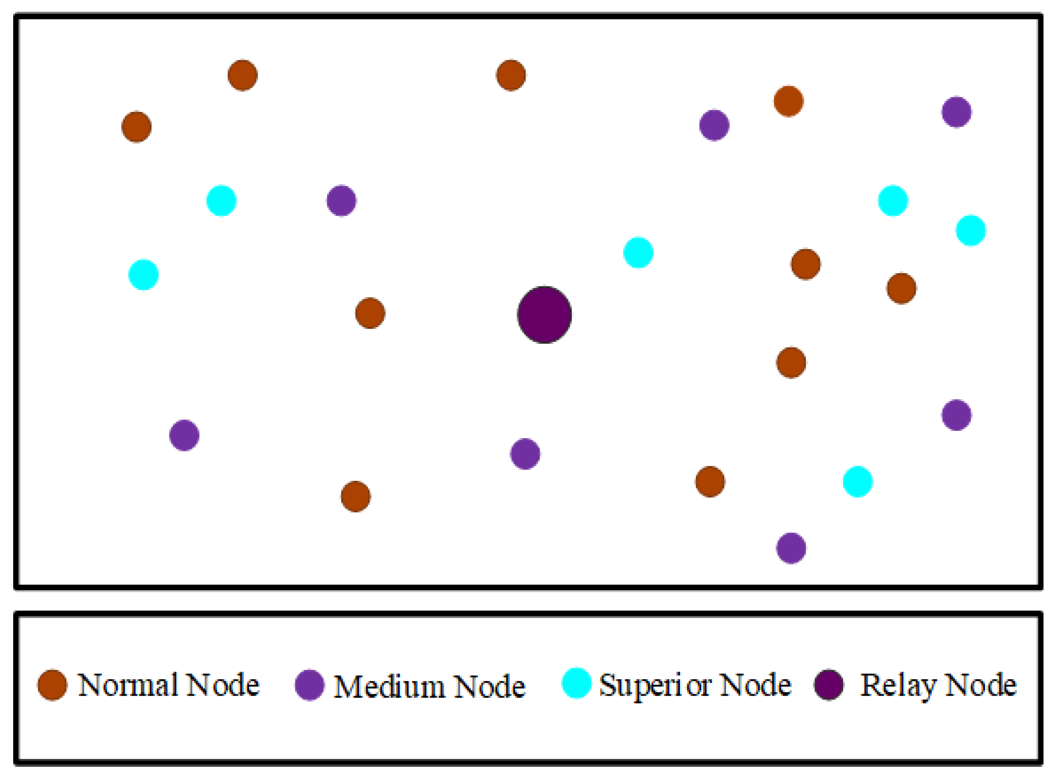
The network model is composed of SNs which are deployed at random over an $M\times M$ network area as illustrated in Figure 1. To analyze the impact of energy heterogeneity, the SNs are divided into three types, which can be adjusted based on real-world scenarios. These three types of SNs are classified as normal, medium, and superior SNs where each type has different levels of initial energies such as superior > medium > normal [38]. This classification reflects the varying battery capacities typically found in different WSN applications. In addition, a RN may be placed in the center of the network. The distance between different SNs, the BS, and the RN can be calculated by using the Global Positioning System (GPS).

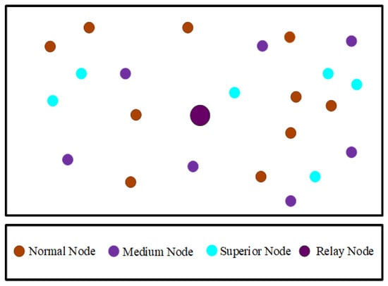
Figure 1. Network relay node and sensor nodes.

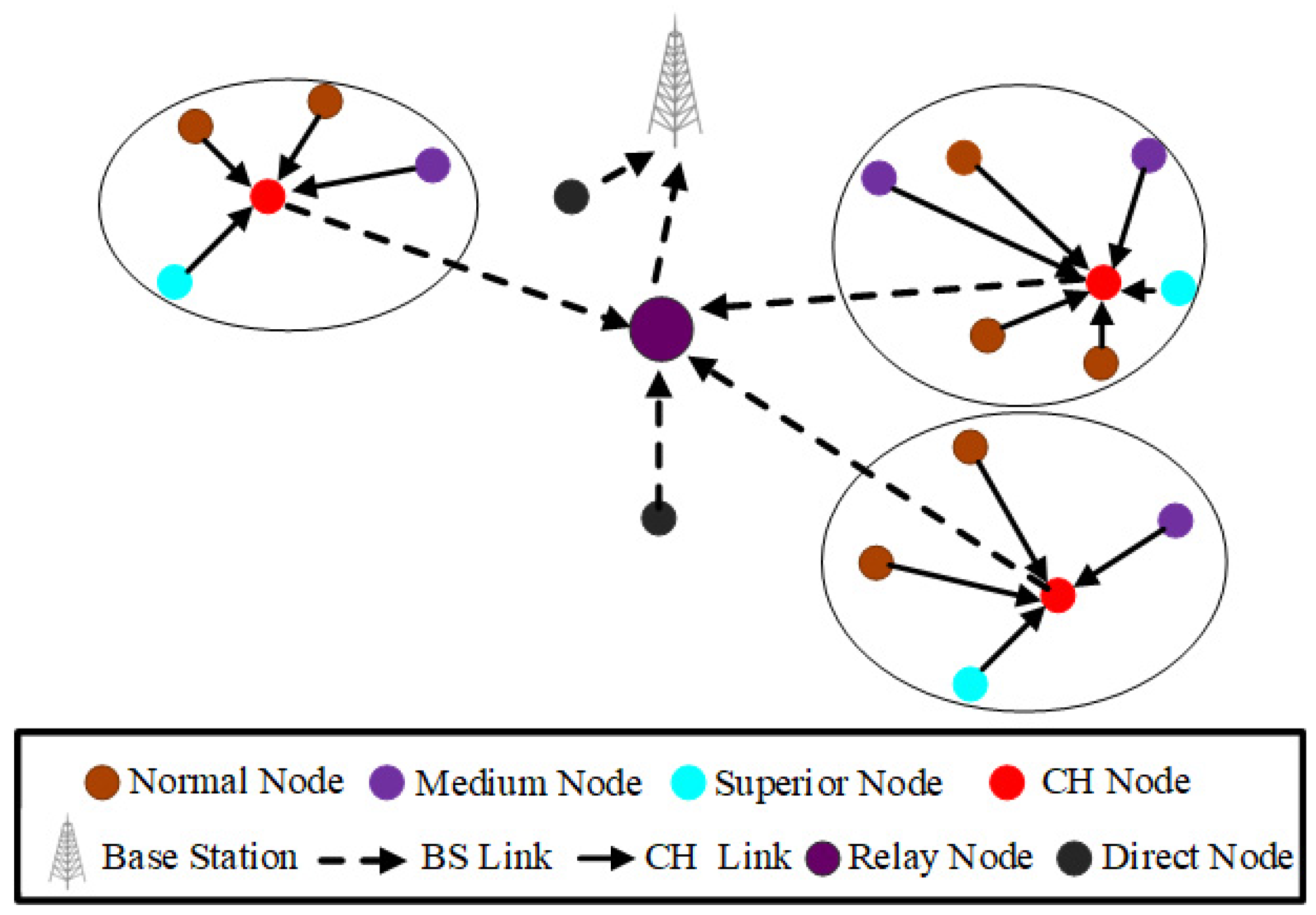
The network operates in two different modes based on the position of the nodes and the clusters as illustrated in Figure 2. In the direct mode, a SN forwards its collected data to a RN or to the BS if the RN or the BS is closer than its CH. In the clustering mode, clusters of SNs transmit data packets to their designated CHs. The CHs, in turn, forward the aggregated data to the RN if the RN is closer than the BS. The RN then transmits the data to the mobile BS which is situated at its optimal location Alternatively, the CHs can directly transmit their data to the BS. Since the BS is assumed to have significantly higher energy reserves compared to the SNs, the energy consumed by the BS during its movement is considered negligible, ensuring efficient network operation.

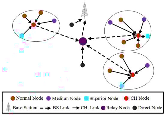
Figure 2. The network model.

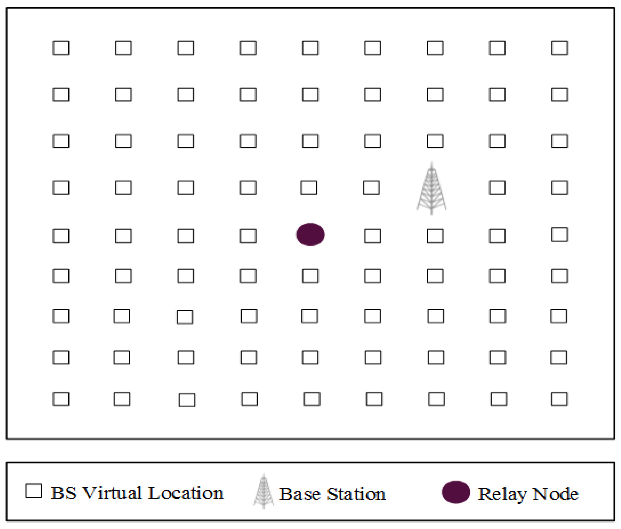
As demonstrated in Figure 3, there is a grid of points for the mobile BS, denoted as the virtual BS points grid, where the mobile BS’s ideal location will be chosen out of all the grid’s points.

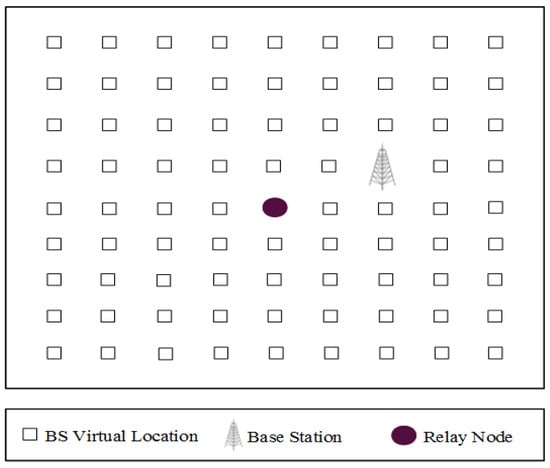
Figure 3. BS virtual points grid.

3.1. Problem Definition

WSNs’ main objective is to balance energy usage and lengthen network longevity. The data transfer procedure from SNs to sinks in WSNs uses the greatest amount of energy. In a WSN deployment, locating the BS far from the SNs leads to reduced network lifespan and significantly higher energy consumption. To address these challenges, the BS must be situated closer to the SNs. Optimizing the BS location can minimize energy consumption, lower operational costs, and reduce network complexity. Given the increasing energy costs and the growing challenges in managing modern IoT, UAV, and WSN systems, efficient energy management is crucial. Our study proposes a novel approach that utilizes a virtual BS points grid to identify the optimal BS location. The grid is designed to minimize the distance parameter, and the best location is dynamically chosen from among the grid points. As SNs begin to deplete their energy and die, the optimization process is repeated to update the BS location, introducing the concept of BS mobility.

In computer science, a mobility model calculates the variations in position, speed, and acceleration of nodes over time. Mobility models can be classified as individual or group-based, depending on whether the nodes move independently or in a correlated manner. In WSNs, mobility models are critical for simulating sensor movement, helping to extend network lifetime, improve coverage, and maintain connectivity. By incorporating these principles, our proposed model aims to enhance the efficiency and sustainability of WSN deployments, with potential applications in other network types. In our model, while all the sensor nodes are stationary, it is assumed that the BS can move in the sensor deployment area based on the calculated grid point.

Furthermore, for large-area WSNs, SNs that are far from BSs will use a lot of energy and eventually die, early; so, to address this issue, the addition of an RN is explored for improving scalability. For large-area WSNs, the data sender and data receiver components have a distance of d. The impact of path loss among the SNs and the base station was examined in the network’s large area. The path loss in the network’s large area grows considering the distance between the SNs and the BS.

3.2. Energy Model

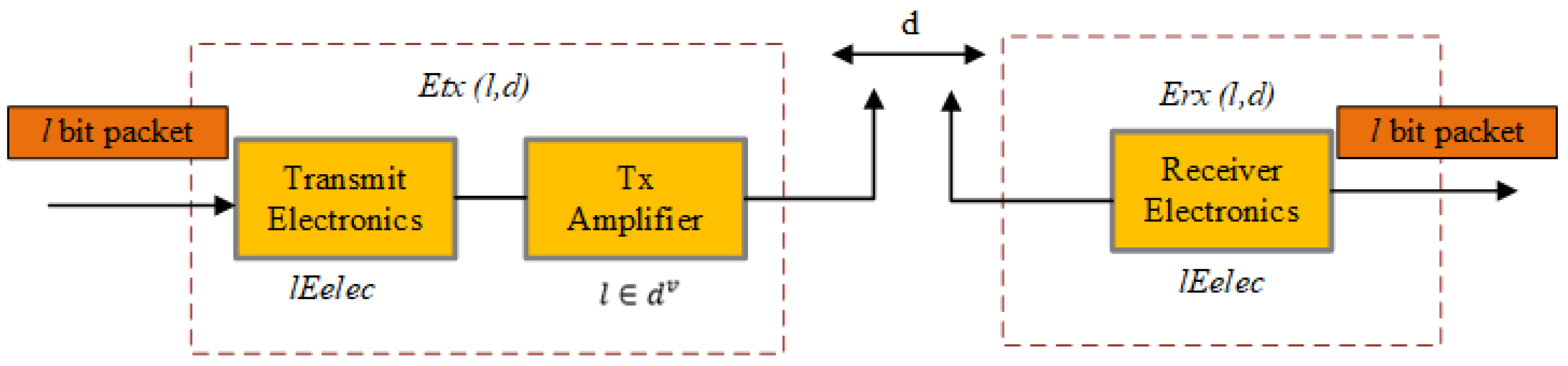
The network energy dissipation model [39], seen in Figure 4, is employed in the proposed model. The energy consumption for sending and receiving a l-bit message across a distance of $d$ is described by Equations (1) and (2).

$$E_{tx}\left(l,d\right)=\left\{\begin{array}{c}l{E}_{elec}+l{\in }_{fs}{d}^2 d\le d_0 \\ l{E}_{elec}+l{\in }_{mp}{d}^4 d>d_0\end{array}\right.$$

(1)

$$E_{rx}\left(l,d\right)=l{E}_{elec}$$

(2)

where ${\mathrm{E}}_{\mathrm{e}\mathrm{l}\mathrm{e}\mathrm{c}}$ represents the power consumed by the sender’s electrical circuits, ${\in }_{\mathrm{f}\mathrm{s}}$ indicates the energy that sensor nodes utilize to send data over free space channels (line of sight), and the energy consumption of data transmission over the multipath channel is ${\in }_{\mathrm{m}\mathrm{p}}$.

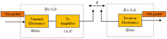
Figure 4. Network energy model.

The threshold distance computation ${\mathrm{d}}_0$ is given in Equation (3)

$$d_0=\sqrt{{\in }_{fs}/{\in }_{mp}}$$

(3)

3.3. Network Operation

For the WSN to operate effectively, rounds are repeated over the entire network lifetime. A round is divided into two stages: the initial setup and the stable state. The clusters are created during the initial setup of each round, while data transfers to the BS occur during the stable state. The duration of the initial setup is shorter than the stable state phase. Every round starts with the initial setup. In the initial setup, clusters are created after CHs are identified. Node election likelihood, threshold perspective, node remaining energy, and the ideal number of clusters are the parameters used in CH picking.

Because heterogeneity has a significant effect on SN networks, we use a heterogeneous network in our model. Here, three types of SNs in a heterogeneous network, named superior, medium, and normal SNs with various initial energies are considered. For superior, medium, and normal SNs, the individual initial energy equations are shown as follows:

$$E_{sup}=E_0\ast (1+b)$$

(4)

$$E_{med}=E_0\ast (1+a)$$

(5)

$$E_{nrm}=E_0$$

(6)

where a and b are the energy extra factors of medium and superior SNs, respectively. ${\mathrm{E}}_0$ is normal SN energy, and ${\mathrm{E}}_{\mathrm{m}\mathrm{e}\mathrm{d}}$ is the medium SN energy, and then ${\mathrm{E}}_{\mathrm{s}\mathrm{u}\mathrm{p}}$ is the superior SN energy and ${\mathrm{E}}_0$ = 0.5, $a$ = 0.45, b = 0.90.

The node selection likelihood for the heterogeneous SNs abides by these guidelines: the superior SN’s likelihood ${\mathrm{p}}_{\mathrm{s}\mathrm{u}\mathrm{p}}$ is larger than the medium SN’s likelihood ${\mathrm{p}}_{\mathrm{m}\mathrm{e}\mathrm{d}}$ and the medium SN’s likelihood is greater than the likelihood of the normal SN’s likelihood ${\mathrm{p}}_{\mathrm{n}\mathrm{r}\mathrm{m}}$, implying that superior and medium SNs have a higher chance of becoming a CH.

$\mathrm{T}\left({\mathrm{n}}_{\mathrm{n}\mathrm{r}\mathrm{m}}\right)$, $\mathrm{T}\left({\mathrm{n}}_{\mathrm{m}\mathrm{e}\mathrm{d}}\right)$, and $\mathrm{T}\left({\mathrm{n}}_{\mathrm{s}\mathrm{u}\mathrm{p}}\right)$ are the thresholds for normal, medium, and superior SNs to become CHs, respectively. The following equation can be used to compute $\mathrm{T}\left({\mathrm{n}}_{\mathrm{n}\mathrm{r}\mathrm{m}}\right)$, $\mathrm{T}\left({\mathrm{n}}_{\mathrm{m}\mathrm{e}\mathrm{d}}\right)$, and $\mathrm{T}\left({\mathrm{n}}_{\mathrm{s}\mathrm{u}\mathrm{p}}\right),$ respectively:

$$T\left(n_{nrm}\right)=\left\{\begin{array}{c}{\displaystyle \frac{p_{nrm}}{1-p_{nrm}(r mod \frac{1}{p_{nrm}})}} if n_{nrm}∊G \\ 0 otherwise\end{array}\right.$$

(7)

$$T\left(n_{med}\right)=\left\{\begin{array}{c}{\displaystyle \frac{p_{med}}{1-p_{med}(r mod \frac{1}{p_{med}})}} if n_{med}∊G \\ 0 otherwise\end{array}\right.$$

(8)

$$T\left(n_{sup}\right)=\left\{\begin{array}{c}{\displaystyle \frac{p_{sup}}{1-p_{sup}(r mod \frac{1}{p_{sup}})}} if n_{sup}∊G \\ 0 otherwise\end{array}\right.$$

(9)

where $\mathrm{r}$ is the iteration number currently in effect, $\mathrm{G}$ is the grouping of SNs that were not chosen in the previous ${\displaystyle \raisebox{1ex}{$1$}\!\left/ \!\raisebox{-1ex}{${\mathrm{p}}_{\mathrm{n}\mathrm{r}\mathrm{m}}$}\right.}$ iteration to be CHs.

In (7), ${\mathrm{p}}_{\mathrm{n}\mathrm{r}\mathrm{m}}$ can be substituted by ${\mathrm{p}}_{\mathrm{m}\mathrm{e}\mathrm{d}}$ and ${\mathrm{p}}_{\mathrm{s}\mathrm{u}\mathrm{p}}$ to obtain $\mathrm{T}\left({\mathrm{n}}_{\mathrm{m}\mathrm{e}\mathrm{d}}\right)$, $\mathrm{T}\left({\mathrm{n}}_{\mathrm{s}\mathrm{u}\mathrm{p}}\right)$. For CH selection, every SN selects a random number ${\mathrm{R}}_{\mathrm{n}}$ from 0 and 1.

In addition to election likelihood, the quantity of energy necessary to obtain, combine, and transfer depends on the number of SNs in the cluster [40]. As a result, the threshold prospective ${\mathrm{E}}_{\mathrm{t}\mathrm{h}}$ is equal to

$$E_{th}=l\left(E_{elec}+E_{da}\right)\left({\displaystyle \frac{N_c}{K_{opt}}}\right)$$

(10)

According to [34], between 5% and 10% of the network’s active SNs should be clustered for optimal energy utilization; as a result, the suitable quantity of CHs is given as

$$K_{opt}=\sqrt{{\displaystyle \frac{N_c}{2\pi }}}\sqrt{{\displaystyle \frac{{\in }_{fs}}{{\in }_{mp}}}} \left({\displaystyle \frac{M}{{d_{toBS}}^{2 }}}\right)$$

(11)

where ${\mathrm{d}}_{\mathrm{t}\mathrm{o}\mathrm{B}\mathrm{S}}$ is the average distance between all CH to BS, $\mathrm{N}\mathrm{c}$ is clustering active SNs.

4. The Optimization of BS Location

One way to improve the longevity and general energy performance of a large WSN network is to add an RN inside the network’s large area, calculate the BS’s suitable location, and move the BS from one desired point to another.

First, we will discuss the impact of the mobile BS-optimized locations in the network large area. The second step will cover introducing an RN in a large-scale WSN. The best point to place the BS is chosen using a new algorithm that considers the distinction in the network’s large region between SNs and BS virtual points in the grid. Let $\mathrm{A}$ be the number of alive SNs, and $\mathrm{V}$ denote the number of BS virtual points. $\mathrm{V}$ is used to find the optimal points ${\mathrm{v}}^{\mathrm{*}}$. Let us define the SN coordinates $\mathrm{n}$ as $(x_n , y_n)$ and the coordinates of the virtual point $\mathrm{v}$ as ($x_v , y_v$). If D is the distance between consecutive virtual points within the grid, the equation below can be used to calculate the number of virtual points within a large network area.

$$\Omega ={({\displaystyle \frac{M}{D}}-1)}^2$$

(12)

The distance between each SN n and virtual point m is illustrated by:

$$d\left(n,v\right)=\sqrt{[{\left(x_n-x_v\right)}^2+{\left(y_n-y_v\right)}^2]}$$

(13)

A weight function ${\mathrm{W}}_{\mathrm{f}}$ is used to establish the computation between alive SNs and virtual point v as follows:

$$W_f=\sum _{n=1}^{S}d\left(n,v\right)$$

(14)

The point that provides the shortest distance from all alive SNs is selected as the best BS location from calculated weights and is given as:

$$v*=\mathit{arg}\mathit{min}\left(W_f\right)$$

(15)

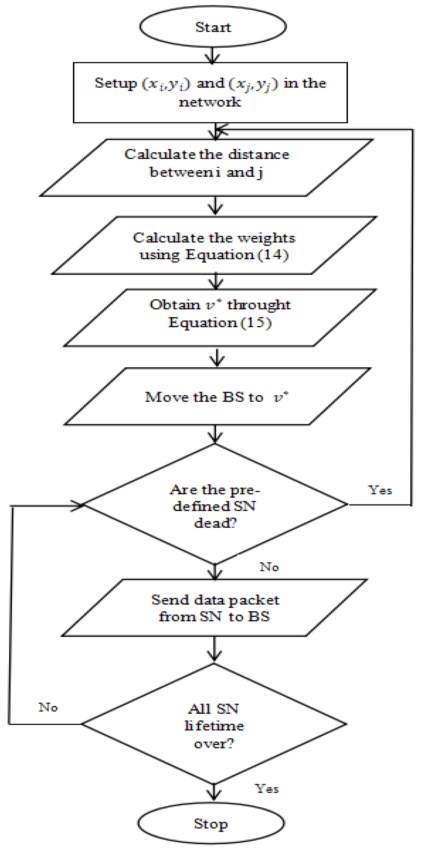
The proposed system enhances the SEP algorithm by introducing a three-tier energy heterogeneity model for SNs, categorizing them as normal, medium, and superior based on their initial energy levels to ensure balanced power consumption. A strategically placed central relay node facilitates efficient data aggregation, while a mobile BS dynamically optimizes communication and reduces energy-intensive transmissions. The modified SEP algorithm calculates the probability of nodes becoming CHs based on their energy levels, with superior nodes having the highest likelihood, followed by medium and normal nodes. This hierarchical energy model, combined with the relay node and mobile BS, reduces energy consumption, evenly distributes the load, and extends the network lifespan. The flowchart in Figure 5 illustrates the integration of these components and demonstrates how the transmission process between SNs and the BS achieves significant energy efficiency improvements.

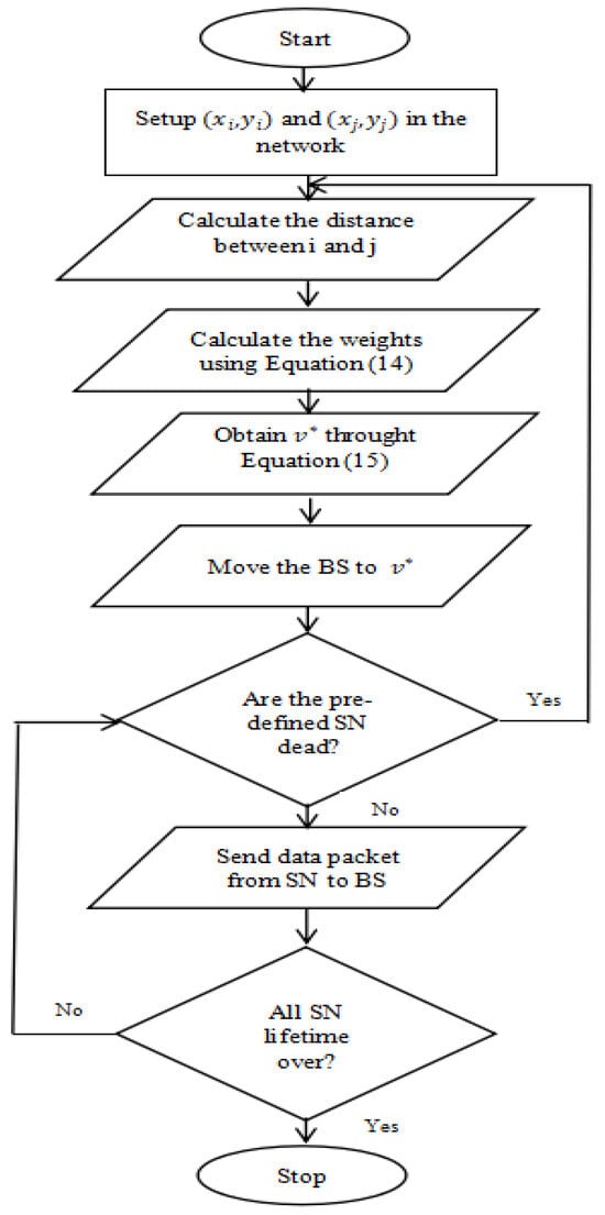
Figure 5. Flowchart of the algorithm.

When the WSN operates in a large deployment area, some of the SNs will die as their energies are depleted. Using the BS suitable location computation, the BS placement can be altered according to the number of alive SNs that are still present. The new best BS location is determined by recalculating the overall distances between each virtual point and the left-alive SNs, subsequently choosing the virtual point with the shortest distance from every SN that is still alive. BS moves to the new location where it can receive sensor node data the best. Algorithm 1 shows the operation of the proposed algorithm without relays. When a relay node R is added to the center of the network large area, the RN receives the data that the CHs have collected if the distance between a CH and the RN is smaller than the distance between the CH and the BS. The RN then resends its collected packets to the BS placed at the optimal location. Algorithm 2 below shows the steps of the proposed algorithm when an RN is added.

We have also examined the impact of path loss on our suggested algorithm. When the packet sender and packet receiver components are separated by a distance of d, the required energy for sending an l-bit message across this distance of d is illustrated below:

$$E_{tx}\left(l,d\right)={l E}_{elec}+l L\left(d\right)$$

(16)

Algorithm 1 Optimization of mobile BS location in a large area network

Set-up the coordinates of SNs ($x_n$, $y_n)$ and virtual points v ($x_m$, $y_m)$ the network Calculate the distance between each live SN and virtual point by Equation (13) Calculate the weights by using Equation (14) Calculate the optimal $l*$ by using Equation (15) Move the BS to $l*$ while the network is alive  if a predefined number of SNs are dead     go to step 2  else     transmit collected data from SNs to BS  end if end while

The path loss $\mathrm{L}\left(\mathrm{d}\right)$ (measured in dB) is approximated by,

$$L \left(d\right)=L_0+10n\times log(d∕ d_0)$$

(17)

where p is the path loss factor, which fluctuates with terrain and surroundings, and $L_0$ is the path loss at an arbitrary reference distance $d_0$.

$$L_0={\in }_{fs}{d_0}^2=7.569\ast {10}^{-8}=-71.20961495 \mathrm{d}\mathrm{B}$$

(18)

To convert the dB value to a normal value the equation will be

$$L \left(d\right)={10}^{{\displaystyle \raisebox{1ex}{$L\left(d\right)dB$}\!\left/ \!\raisebox{-1ex}{$10$}\right.}}$$

(19)

By placing the path loss, given in Equation (16) the required energy for sending an l-bit message across a distance d will be computed as

$$E_{tx}\left(l,d\right)={lE}_{elec}+l\ast {10}^{{\displaystyle \raisebox{1ex}{$L\left(d\right)dB$}\!\left/ \!\raisebox{-1ex}{$10$}\right.}}$$

(20)

Algorithm 2 Optimization of mobile BS location in a large area network with a RN

Set-up the coordinates of SNs ($x_n$, $y_n)$ and virtual points v ($x_m$, $y_m)$ the network Calculate the distance between each live SN and virtual point by Equation (13) Calculate the weights by using Equation (14) Calculate the optimal $l^{*}$ by using Equation (15) Move the BS to $l^{*}$ while the network is alive    if a predefined number of SNs are dead     go to step 2    else if     transmit collected data to RN, and RN will retransmit data to BS    else     transmit collected data to the BS directly    end if end while

5. Simulation Results

Under the objective of the analysis and comparison of the proposed algorithms, we used MATLAB for the simulation studies and evaluated the proposed algorithms’ performances. The parameters utilized in the simulations are given in Table 1. To observe the network lifetimes and remaining network energies, the simulations are conducted up to 3500 rounds. After each 5% SN death, the optimal mobile BS location on the grid is calculated and the mobile BS moved to the calculated position.

Table 1. The parameters of the simulation.

Parameters	Values
Size of network	$100 \mathrm{m}\times 100 \mathrm{m}$
Number of sensor nodes (S)	100
Election probability value of CH $(p$)	0.1
Coefficient for amplification signal from free space (${\in }_{\mathrm{f}\mathrm{s}}$)	10 PJ/bit/${\mathrm{m}}^2$
Signal amplification coefficient of multi-path fading (${\in }_{mp}$)	0.0013 PJ/bit/${\mathrm{m}}^4$
Energy consumption in electronic circuitry (${\mathrm{E}}_{elec}$)	50 nJ/bit
Energy consumption in data aggregation (${\mathrm{E}}_{DA}$)	5 nJ/bit
Packet size	4000 bits

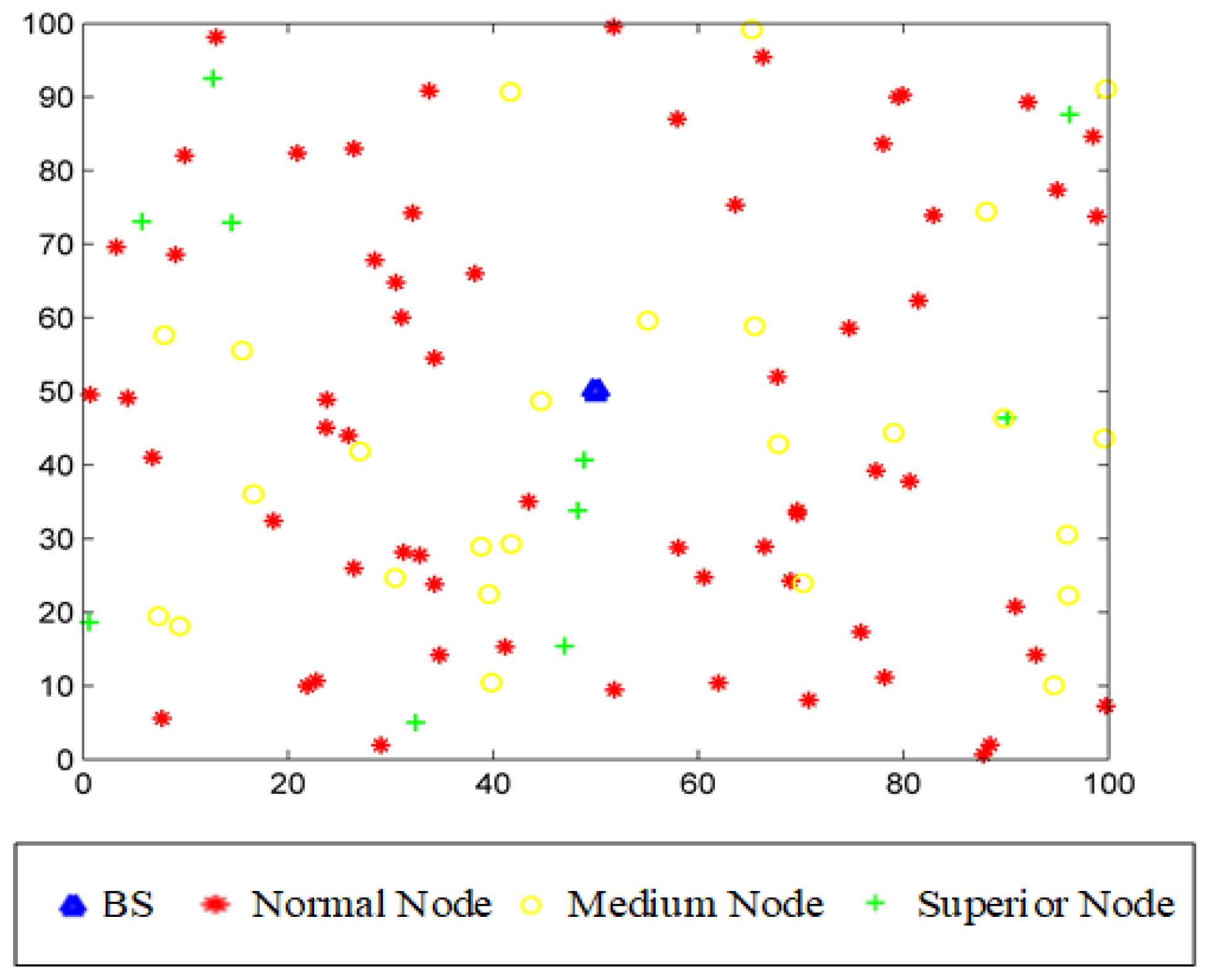
To illustrate our simulations, an instance of 100 scattered SNs followed up by GPS in a 100 m × 100 m heterogeneous network field is shown in Figure 6. The mobile BS is located at the center of the sensor deployment area at the beginning of the simulation. For example, if the sensors are deployed in a size $M\times M$ area, the BS is located at coordinates $\left({\displaystyle \frac{M}{2}},{\displaystyle \frac{M}{2}}\right)$ at the start of the simulation.

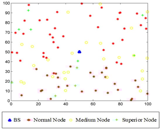
Figure 6. An illustration of a 100 m × 100 m sensor network field.

10% of the nodes are assumed to be superior SNs, which have the highest initial energy levels in the network. 15% of the nodes are assumed to be medium SNs, which have the medium initial energy levels in the network. The remaining 75% of the nodes are assumed to be normal SNs, which have the lowest initial energy levels in the network. As each SN has a chance to be elected as a CH, all SNs can aggregate data that they receive from other SNs including their own collected data.

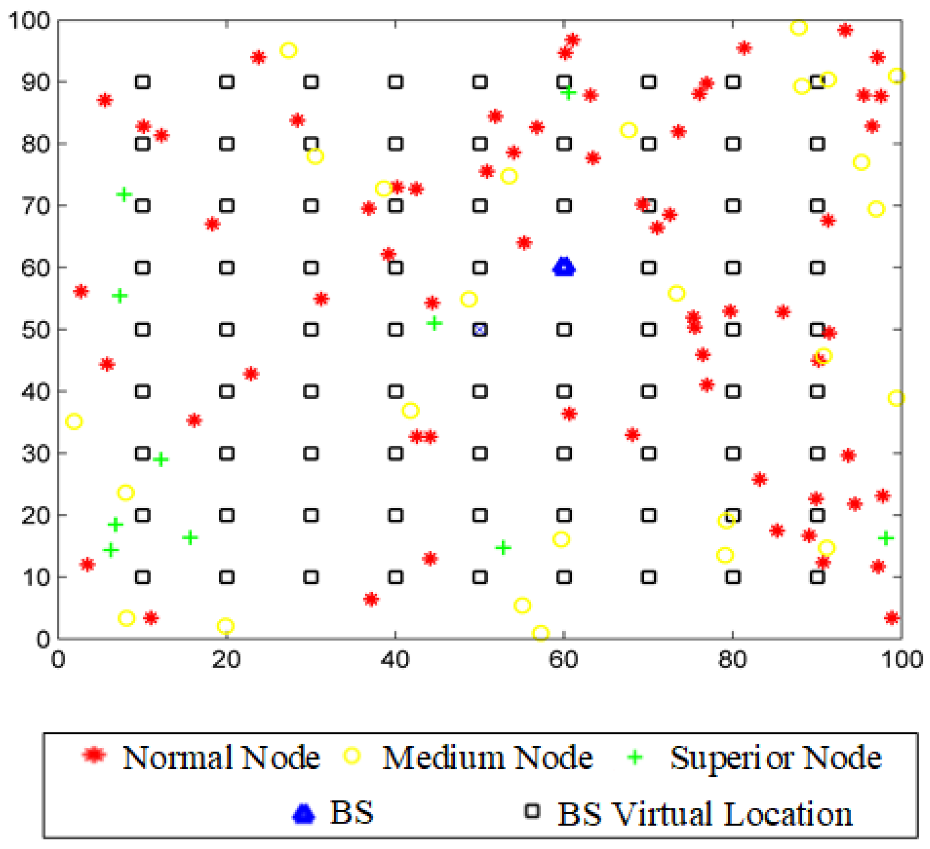
In the sensor network field, the separation between adjacent BS virtual points in the grid is set to be 10 m. The BS virtual points on the edges of the sensor network field are omitted. Therefore, in a 100 m × 100 m network field, there are 81 BS virtual points. At a particular time during the simulation, the optimum BS location which has the shortest overall distance from all active SNs, can be one of these virtual points.

Figure 7 illustrates an instance of the sensor network field with the BS virtual points. At this instance, the mobile BS is positioned at coordinates $\left(\mathrm{60,60}\right)$. For each 5% SN death, the proposed algorithm recalculates the optimal BS location on the grid and the mobile BS moves to that point to collect the data from the remaining alive SNs. Throughout the lifetime of the network, this procedure referred to as the BS mobility is repeated.

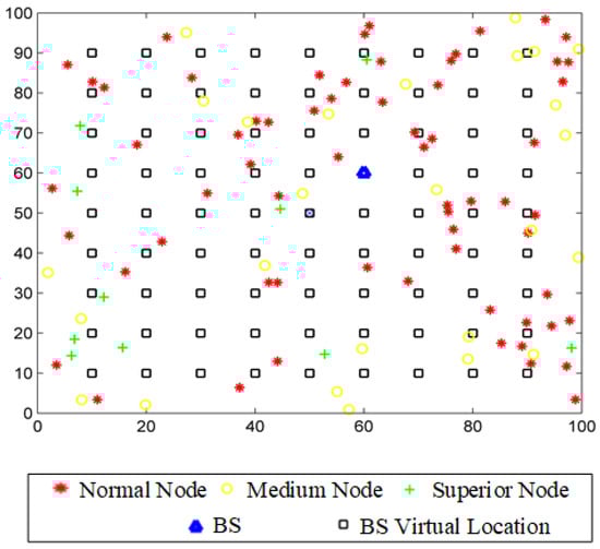
Figure 7. An illustration of a 100 m × 100 m sensor network field with BS virtual locations.

5.1. Optimal BS Location and BS Mobility in a Large Area Network

In this Section, the effectiveness of the suggested algorithm in a large-area network regarding network lifetime and residual energy is discussed. In the simulations, 400 SNs are scattered in a $400 \mathrm{m}\times 400 \mathrm{m}$ sensor network field. When the proposed algorithm is applied on the SEP protocol utilizing two and three energy levels (SEPWMBS and SEPWMBS-3L) in a large-area network, their resulting network lifetimes as well as the network lifetimes of the conventional SEP protocol utilizing two and three energy levels (SEP and SEP-3L) are shown in Figure 8. It can be observed that SEPWMBS improves the lifetime of SEP and SEPWMBS-3L improves the lifetime of SEP3 significantly.

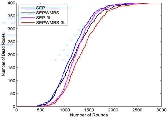
Figure 8. Comparison of network lifetimes in a large area network.

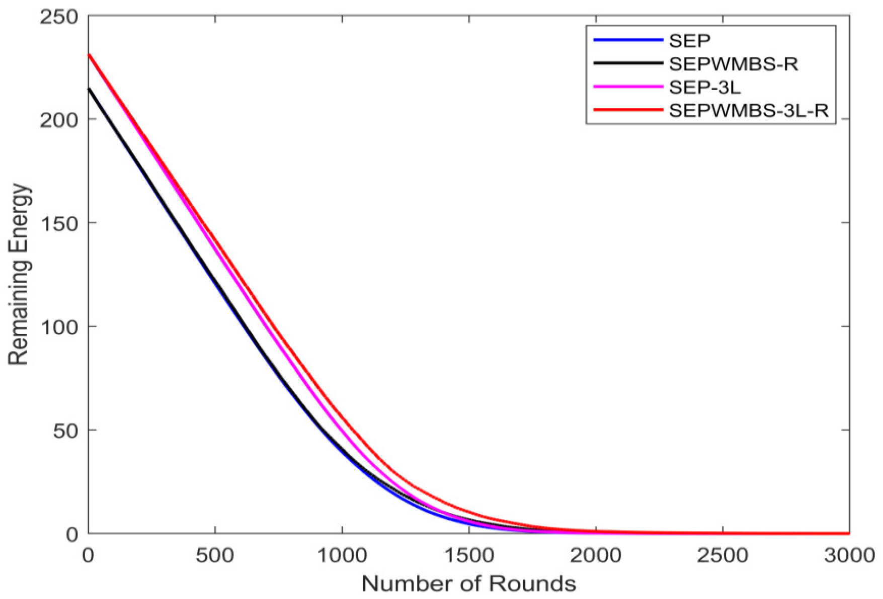
In Figure 9, the total remaining network energy is presented for the above-mentioned protocols. The network’s energy is completely depleted under SEPWMBS and SEPWMBS-3L at rounds 2585 and 2701, respectively. Whereas underneath SEP and SEP-3L, the network’s energy is completely depleted at rounds 2342 and 2452, respectively. Therefore, the usage of mobile BS improves the lifetime of SEP by 243 rounds and SEP-3L by 249 rounds. These results demonstrate that the proposed algorithm can reduce the energy consumption of the network better when compared with SEP.

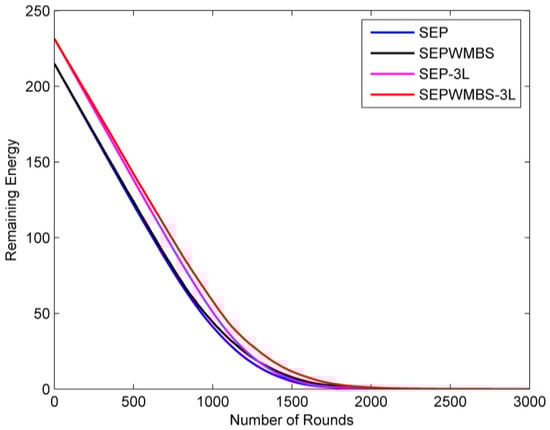
Figure 9. Comparison of remaining energies in a large area network.

5.2. Placement of the RN

In order to observe the impact of the RN on the lifetime of the sensor network, a RN is positioned at the center of the sensor network field. When a RN is implemented, the CHs can transmit their collected data to the RN, if better energy conservation can be achieved. The RN will then transmit the collected data to the BS. In this part, the simulation outcomes with RN are presented.

As presented in Figure 10, when a RN is used, the network lifetimes with the proposed algorithm over SEP protocol utilizing two and three energy levels (SEPWMBS-R and SEPWMBS-3L-R) are almost 2603 and 2832 rounds, respectively. In the conventional SEP protocol utilizing two and three energy levels (SEP and SEP-3L), the network lifetimes are approximately 2481 and 2502 rounds, respectively. Since the usage of a RN helps reduce the overall communication distances between the SNs and the BS, the network lifetimes increase when compared to the case without using a RN.

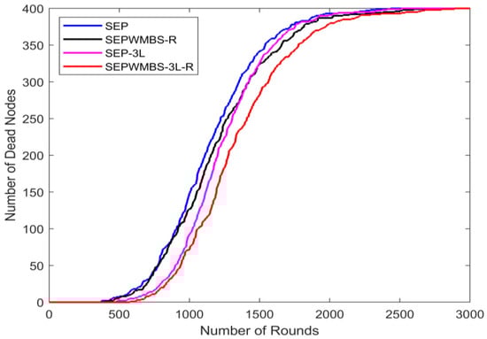
Figure 10. Comparison of network lifetimes in a large area network with a RN.

A comparison of remaining energies in a large area network when a relay node is used is illustrated in Figure 11. While for SEPWMBS-R and SEPWMBS-3L-R, the network energies are completely depleted at rounds 2653 and 2823, respectively, under the conventional SEP and SEP-3L protocols, the total energy depletion occurs at rounds 2473 and 2653 rounds, respectively. These results are promising as they imply that RN usage may improve the overall energy efficiency of a WSN.

Figure 11. Comparison of remaining energies in a large area network with a RN.

5.3. The Path Loss Effect

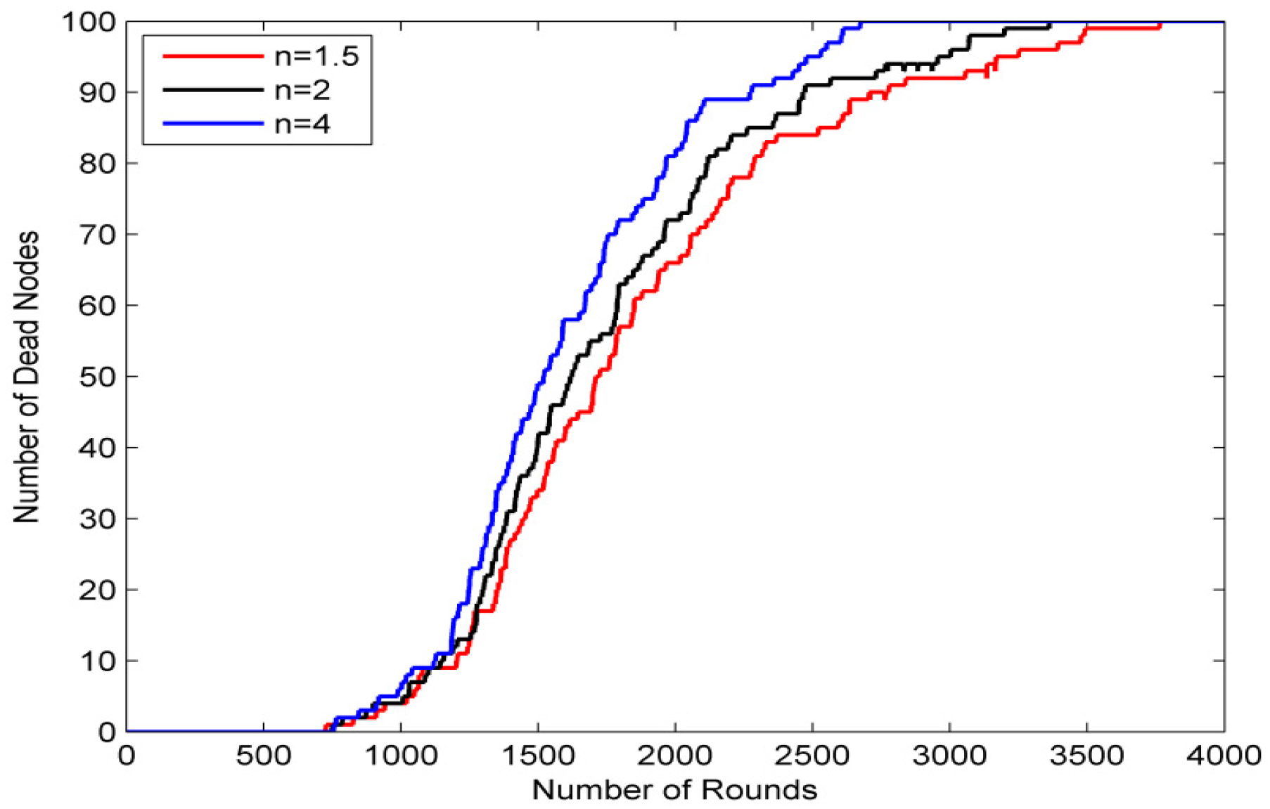
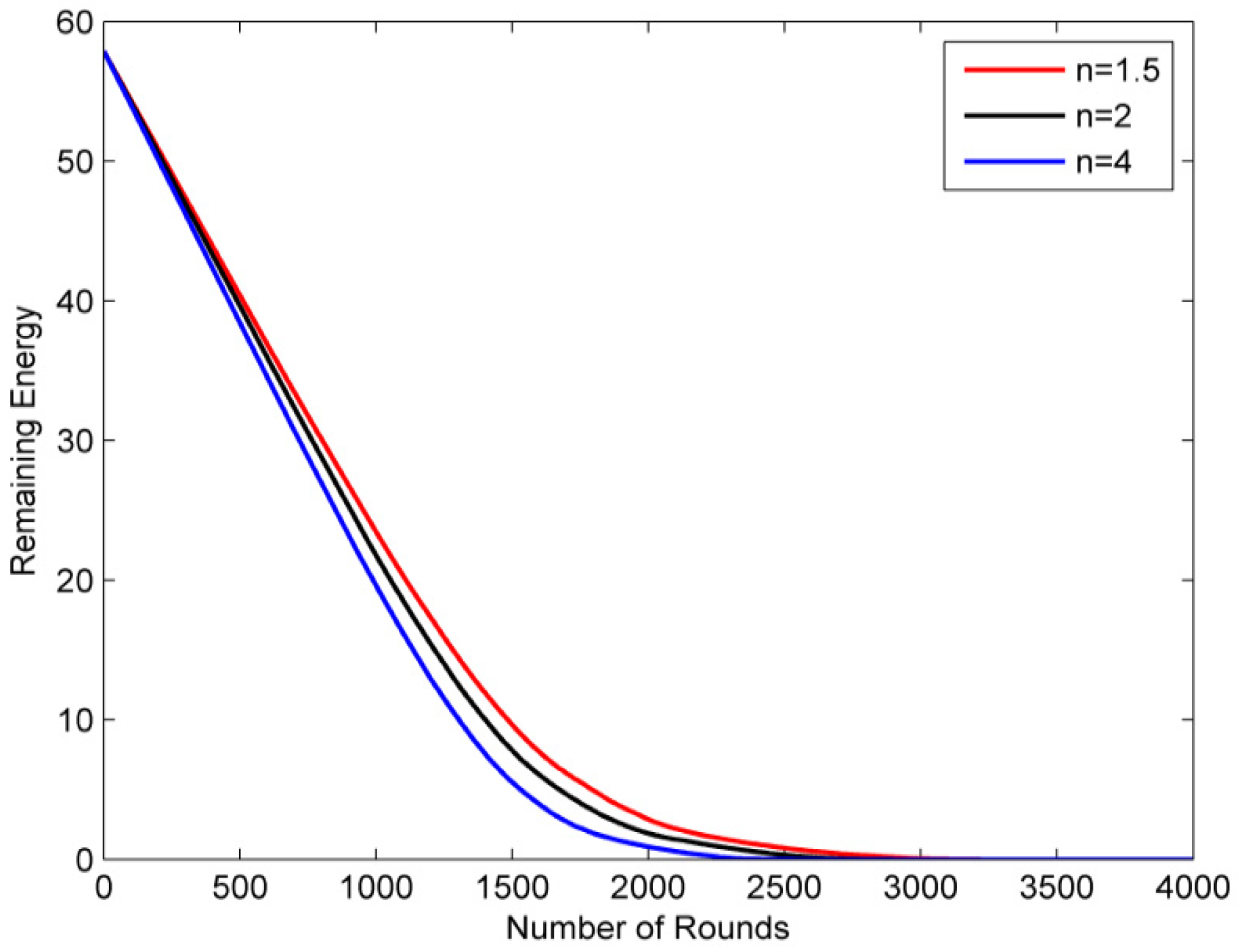
In this part of the simulation studies, the impact of path loss exponent on the network is analyzed. For the studies, the path loss exponent values of n = 1.5, 2 and 4 are used. Figure 12 and Figure 13 illustrate the impact on network lifetime and remaining energy.

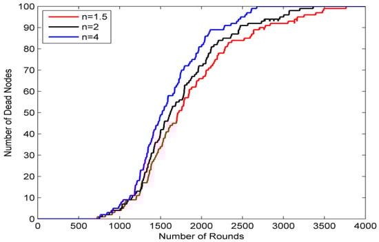
Figure 12. The impact of the path loss exponent on the network lifetime.

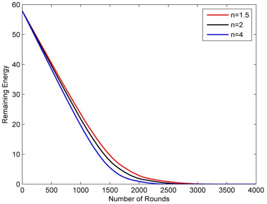
Figure 13. The impact of the path loss exponent on the network’s remaining energy.

As shown in Figure 12, the network lifetimes are approximately 3786, 3423, and 2582 rounds when path loss exponent values are 1.5, 2, and 4 respectively. These results indicate that an increase in the path loss exponent value leads to a significant decrease in the network lifetime.

The impact of the path loss exponent on the network’s remaining energy is illustrated in Figure 13. For the path loss exponent values of 1.5, 2, and 4, the network energy is completely depleted at rounds 3752, 3410, and 2574, respectively. This confirms the fact that increasing the path loss exponent value reduces the lifetime of the network as the nodes consume more energy to transmit their data to the BS.

6. Conclusions

WSNs deployed over large areas face significant challenges due to the limited energy resources of the SNs. Data transmission over long distances between SNs and the BS leads to rapid energy depletion. In this study, we proposed an algorithm for dynamically optimizing the BS location using a virtual grid approach. The algorithm relocates the BS to an optimal position after a number of rounds, accounting for the number of active SNs in the network.

Additionally, we investigated the integration of a RN to improve scalability and energy efficiency in large networks. The proposed algorithms were applied to the conventional SEP protocol with two and three energy levels, and their performance was evaluated in terms of network lifetime and residual energy. Simulation results demonstrated that dynamically adjusting the BS location significantly enhances network performance in large-scale deployments. The inclusion of an RN further increases energy efficiency by reducing transmission burdens on SNs farthest from the BS.

Finally, the study examined the impact of path loss between SNs and the BS, showing that energy consumption increases as the path loss exponent value increases. The findings highlight the importance of optimized BS placement and RN utilization in mitigating energy loss and extending the operational lifetime of WSNs.

References

- Kavre, M.; Gadekar, A.; Gadhade, Y. Internet of Things (IoT): A Survey. In Proceedings of the 2019 IEEE Pune Section International Conference (PuneCon), Pune, India, 18–20 December 2019; pp. 1–6. [Google Scholar]
- John, A.; Rajput, A.; Babu, K.V. Energy saving cluster head selection in wireless sensor networks for internet of things applications. In Proceedings of the 2017 International Conference on Communication and Signal Processing (ICCSP), Chennai, India, 6–8 April 2017; pp. 34–38. [Google Scholar]
- Zannou, A.; Boulaalam, A.; Nfaoui, E.H. An Optimal Base Stations Positioning for the Internet of Things Devices. In Proceedings of the 2021 7th International Conference on Optimization and Applications (ICOA), Wolfenbüttel, Germany, 19–20 May 2021; pp. 1–5. [Google Scholar]
- Sadrishojaei, M.; Navimipour, N.J.; Reshadi, M.; Hosseinzadeh, M. A New Preventive Routing Method Based on Clustering and Location Prediction in the Mobile Internet of Things. IEEE Internet Things J. 2021, 8, 10652–10664. [Google Scholar] [CrossRef]
- Thangarasu, G.; Dominic, P.D.D.; Subrmanian, K.; Kayalvizhi, S.; Masillamony, S.S. Efficient Energy Usage Model for WSN-IoT Environments. In Proceedings of the 2020 International Conference on Computational Intelligence (ICCI), Bandar Seri Iskandar, Malaysia, 8–9 October 2020; pp. 252–255. [Google Scholar]
- Yetgin, H.; Cheung, K.T.K.; El-Hajjar, M.; Hanzo, L.H. A Survey of Network Lifetime Maximization Techniques in Wireless Sensor Networks. IEEE Commun. Surv. Tutor. 2017, 19, 828–854. [Google Scholar] [CrossRef]
- He, S.; Dai, Y.; Zhou, R.; Zhao, S. A Clustering Routing Protocol for Energy Balance of WSN based on Genetic Clustering Algorithm. IERI Procedia 2012, 2, 788–793. [Google Scholar] [CrossRef]
- Lata, S.; Mehfuz, S.; Urooj, S. Secure and Reliable WSN for Internet of Things: Challenges and Enabling Technologies. IEEE Access 2021, 9, 161103–161128. [Google Scholar] [CrossRef]
- Shabbir, N.; Hassan, S. Routing Protocols for Wireless Sensor Networks (WSNs). Wireless Sensor Networks Insights and Innovations; IntechOpen: London, UK, 2017. [Google Scholar] [CrossRef]
- Singh, A.K.; Bhalla, A.; Kumar, P.; Kaushik, M. Hierarchical routing protocols in WSN: A brief survey. In Proceedings of the 2017 3rd International Conference on Advances in Computing, Communication and Automation (ICACCA) (Fall), Dehradun, India, 15–16 September 2017; pp. 1–6. [Google Scholar]
- Toor, A.S.; Jain, A.K. A survey of routing protocols in Wireless Sensor Networks: Hierarchical routing. In Proceedings of the 2016 International Conference on Recent Advances and Innovations in Engineering (ICRAIE), Jaipur, India, 23–25 December 2016; pp. 1–6. [Google Scholar]
- Mishra, P.K.; Verma, S.K. A survey on clustering in wireless sensor network. In Proceedings of the 2020 11th International Conference on Computing, Communication and Networking Technologies (ICCCNT), Kharagpur, India, 1–3 July 2020; pp. 1–5. [Google Scholar]
- Verma, P.; Shaw, S.; Mohanty, K.; Richa, P.; Sah, R.; Mukherjee, A. A Survey on Hierarchical Based Routing Protocols for Wireless Sensor Network. In Proceedings of the 2018 International Conference on Communication, Computing and Internet of Things (IC3IoT), Chennai, India, 15–17 February 2018; pp. 338–341. [Google Scholar]
- Sharma, D.K.; Bagga, S.; Rastogi, R. Performance Analysis of Clustering Based Routing Protocols in Wireless Sensor Networks. In Proceedings of the 2018 3rd International Conference on Contemporary Computing and Informatics (IC3I), Gurgaon, India, 10–12 October 2018; pp. 68–75. [Google Scholar]
- Sampoornam, K.P.; Saranya, S.; Mohanapriya, G.K.; Sandhiya Devi, P.; Dhaarani, S. Analysis of LEACH Routing Protocol in Wireless Sensor Network with Wormhole Attack. In Proceedings of the 2021 Third International Conference on Intelligent Communication Technologies and Virtual Mobile Networks (ICICV), Tirunelveli, India, 4–6 February 2021; pp. 147–152. [Google Scholar]
- Abbas, S.S.A.; Dag, T.; Gucluoglu, T. Increasing Energy Efficiency of WSNs Through Optimization of Mobile Base Station Locations. In Proceedings of the 2021 29th Signal Processing and Communications Applications Conference (SIU), Istanbul, Turkey, 9–11 June 2021; pp. 1–4. [Google Scholar]
- Priyadarshi, R.; Singh, R.L.; Singh, A. A Novel HEED Protocol for Wireless Sensor Networks. In Proceedings of the 2018 5th International Conference on Signal Processing and Integrated Networks (SPIN), Noida, India, 22–23 February 2018; pp. 296–300. [Google Scholar]
- Vugar; Nazila Performance Analysis of LEACH, SEP and Z-SEP Protocols in Heterogeneous Wireless Sensor Network. Wasit J. Comput. Math. Sci. 2023, 2, 27–37. [CrossRef]
- Latiff, N.A.; Ismail, I. Performance of mobile base station using Genetic Algorithms in Wireless Sensor Networks. In Proceedings of the 2016 German Microwave Conference (GeMiC), Bochum, Germany, 14–16 March 2016; pp. 251–254. [Google Scholar]
- Abushiba, W.; Johnson, P.; Alharthi, S.; Wright, C. An energy efficient and adaptive clustering for wireless sensor network (CH-leach) using leach protocol. In Proceedings of the 2017 13th International Computer Engineering Conference (ICENCO), Cairo, Egypt, 27–28 December 2017; pp. 50–54. [Google Scholar] [CrossRef]
- Nguyen, L.; Nguyen, H.T. Mobility based network lifetime in wireless sensor networks: A review. Comput. Netw. 2020, 174, 107236. [Google Scholar] [CrossRef]
- Tseng, Y.; Hwang, R.; Lai, C.; Hou, C. Optimal Sink Placement in M2M over LTE Networks. In Proceedings of the 2015 IEEE International Conference on Smart City/SocialCom/SustainCom (SmartCity), Chengdu, China, 19–21 December 2015; pp. 135–140. [Google Scholar]
- Li, X.; Cai, H.; Liu, G.; Lu, K. Base Station Positioning in Single-Tiered Wireless Sensor Networks. In Proceedings of the 2019 20th International Conference on Parallel and Distributed Computing, Applications and Technologies (PDCAT), Gold Coast, Australia, 5–7 December 2019; pp. 7–12. [Google Scholar]
- Prabha, M.; Darly, S.; Rabi, B.J. Energy conservative mobile sink path routing for wireless sensor networks. In Proceedings of the 2019 International Conference on Smart Structures and Systems (ICSSS), Chennai, India, 14–15 March 2019; pp. 1–6. [Google Scholar]
- Kumar, A.R.; Sivagami, A. Energy Aware Localized Routing in Rendezvous Point Based Mobile Sink Strategy for Wireless Sensor Networks. In Proceedings of the 2019 Innovations in Power and Advanced Computing Technologies (i-PACT), Vellore, India, 22–23 March 2019; pp. 1–6. [Google Scholar]
- Zhou, R. Research on Efficiency Optimization of Logistics Vehicle Monitoring Model Based on Wireless Sensor Network. J. ICT Stand. 2023, 11, 27–44. [Google Scholar] [CrossRef]
- Haripriya, R.; Vinutha, C.B.; Shoba, M. Genetic Algorithm with Bacterial Conjugation Based Cluster Head Selection for Dynamic WSN. In Proceedings of the 2023 International Conference on Network, Multimedia and Information Technology (NMITCON), Bengaluru, India, 1–2 September 2023; pp. 1–6. [Google Scholar]
- Shah, I.K.; Maity, T.; Dohare, Y.S. Weight Based Approach for Optimal Position of Base Station in Wireless Sensor Network. In Proceedings of the 2020 International Conference on Inventive Computation Technologies (ICICT), Coimbatore, India, 26–28 February 2020; pp. 734–738. [Google Scholar]
- Mitra, R.; Sharma, S. Proactive data routing using controlled mobility of a mobile sink in Wireless Sensor Networks. Comput. Electr. Eng. 2018, 70, 21–36. [Google Scholar] [CrossRef]
- Hassan, A.A.-H.; Shah, W.M.; Habeb, A.-H.H.; Othman, M.F.I.; Al-Mhiqani, M.N. An Improved Energy-Efficient Clustering Protocol to Prolong the Lifetime of the WSN-Based IoT. IEEE Access 2020, 8, 200500–200517. [Google Scholar] [CrossRef]
- Pitchaimanickam, B.; Muthuvel, P.; Rajasekar, R. Multi-Verse Optimization for Node Localization in Wireless Sensor Networks. In Proceedings of the 2024 Third International Conference on Electrical, Electronics, Information and Communication Technologies (ICEEICT), Trichirappalli, India, 24–26 July 2024; pp. 1–5. [Google Scholar]
- Wang, X.; Zhou, Q.; Qu, C.; Chen, G.; Xia, J. Location Updating Scheme of Sink Node Based on Topology Balance and Reinforcement Learning in WSN. IEEE Access 2019, 7, 100066–100080. [Google Scholar] [CrossRef]
- Tirani, S.P.; Avokh, A. On the performance of sink placement in WSNs considering energy-balanced compressive sensing-based data aggregation. J. Netw. Comput. Appl. 2018, 107, 38–55. [Google Scholar] [CrossRef]
- Abrishambaf, R.; Bal, M. Base station positioning for industrial wireless sensors. In Proceedings of the 2018 IEEE International Conference on Consumer Electronics (ICCE), Las Vegas, NV, USA, 12–14 January 2018; pp. 1–4. [Google Scholar]
- Jindal, V.; Jha, A.; Goel, K.; Jha, V. Improving Network Lifetime and Area Coverage with Optimal Sink Mobility Pattern and Node Deployment Strategy in WSN. In Proceedings of the 2018 12th International Conference on Signal Processing and Communication Systems (ICSPCS), Cairns, Australia, 17–19 December 2018; pp. 1–10. [Google Scholar]
- Shahraki, A.; Taherkordi, A.; Haugen, Ø.; Eliassen, F. Clustering objectives in wireless sensor networks: A survey and research direction analysis. Comput. Netw. 2020, 180, 107376. [Google Scholar] [CrossRef]
- Radha, S.; Bala, G.J.; Rajkumar, N.P.; Indumathi, G.; Nagabushanam, P. Optimal relay nodes placement with game theory optimization for Wireless Sensor Networks. J. High Speed Netw. 2024, 29–51. [Google Scholar] [CrossRef]
- Yodianto, W.; Warnars, H.L.H.S.; Warnars, L.L.H.S.; Ramadhan, A.; Siswanto, T. Searching Routing using A-Star (A*) Search Algorithm. In Proceedings of the 2024 3rd International Conference on Creative Communication and Innovative Technology (ICCIT), Tangerang, Indonesia, 7–8 August 2024; pp. 1–7. [Google Scholar]
- Smaragdakis, G.; Matta, I.; Bestavros, A. SEP: A Stable Election Protocol for Clustered Heterogeneous Wireless Sensor Networks. In Proceedings of the Second International Workshop on Sensor and Actor Network Protocols and Applications (SANPA 2004), Boston, MA, USA, 22 August 2004. [Google Scholar]
- Panchal, A.; Singh, L.; Singh, R.K. RCH-LEACH: Residual Energy based Cluster Head Selection in LEACH for Wireless Sensor Networks. In Proceedings of the 2020 International Conference on Electrical and Electronics Engineering (ICE3), Gorakhpur, India, 14–15 February 2020; pp. 322–325. [Google Scholar]
Disclaimer/Publisher’s Note: The statements, opinions and data contained in all publications are solely those of the individual author(s) and contributor(s) and not of MDPI and/or the editor(s). MDPI and/or the editor(s) disclaim responsibility for any injury to people or property resulting from any ideas, methods, instructions or products referred to in the content. |
© 2025 by the authors. Licensee MDPI, Basel, Switzerland. This article is an open access article distributed under the terms and conditions of the Creative Commons Attribution (CC BY) license (https://creativecommons.org/licenses/by/4.0/).