Article

The Approach of Using a Horizontally Layered Soil Model for Inhomogeneous Soil, by Taking into Account the Deeper Layers of the Soil, and Determining the Model’s Parameters Using Evolutionary Methods

Faculty of Electrical Engineering and Computer Science, University of Maribor, Koroška Cesta 46, 2000 Maribor, Slovenia
*
Author to whom correspondence should be addressed.
Appl. Sci. 2025, 15(3), 1420; https://doi.org/10.3390/app15031420
Submission received: 20 December 2024 / Revised: 20 January 2025 / Accepted: 26 January 2025 / Published: 30 January 2025
(This article belongs to the Collection Heuristic Algorithms in Engineering and Applied Sciences)

Abstract

:

Featured Application

Larger grounding systems are often designed using the finite element method. A finite element method model can only be made if the data of the soil structure are known in advance. A problem arises when the soil is not homogeneous and the horizontally layered soil model poorly represents the actual conditions in the soil. This paper introduces an approach that describes the use of an analytical horizontally layered soil model for inhomogeneous soil. In this approach, deeper layers of the soil are also considered, which are enabled using higher distances d in Wenner’s method, as in the case of simply dividing the area into smaller parts. Our approach is unique.

Abstract

A new approach using a horizontally layered analytical soil model for inhomogeneous soil is presented. The presented approach also considers deeper soil layers, which is not the case when simply dividing the area of interest into smaller subareas. The finite element method model was used to prepare test data because, in such a case, the soil parameters are known. Six lines simulating Wenner’s method were used, and their results were combined appropriately to determine the soil parameters of nine subareas. To determine the soil parameters in the scope of each subarea, different optimization methods were used and compared to each other. The results were analyzed, and Artificial Bee Colony was selected as the most appropriate method among those tested. Additionally, the convergence of the methods was analyzed, and Memory Assistance is presented, with the aim of shortening the calculation time. In this study, three-, four-, five-, and six-layered soil models were tested, and it is concluded that the three-layered model is most appropriate. A finite element method model based on the soil determination results was constructed to verify the results. The results of the Wenner’s method simulation in the cases of the test data and final model were compared to confirm the accuracy of the presented method.

1. Introduction

The safety of electric devices connected to a network depends on the appropriate dimensioning of the grounding systems. In the case of a technical failure or lightning strike, it is the grounding system that ensures the safety of people and animals. This means that the step voltage and touch voltage should not increase beyond the limit permitted by the standard. Larger grounding systems are often designed using the finite element method (FEM) [1,2,3,4,5,6,7,8,9,10,11,12]. With the FEM model, the potential distribution in and on the soil’s surface can be determined, and the step voltage and touch voltage are determined based on the calculated potentials.
An FEM model can only be made if the data of the soil structure are known in advance. This information is usually obtained through measurements. Various measurement methods are used, the most common of which is the Wenner method [13,14,15,16,17]. A generalized method can also be found in the literature [14], and the Schlumberger method is also mentioned in [17]. This article focuses on the Wenner method.
Determining the parameters of the soil is a difficult task because it requires an inverse approach. Analytical horizontal multi-layer soil models [15,16,17,18,19] are of great help in this task. The soil data are obtained using the Wenner method, in which the apparent resistivity is determined for different electrode spacings. It is necessary to determine such parameters of analytical models of soil with two or more layers [15,16,17,18,19] so that the calculated resistances coincide with the measured ones. Due to the complexity of the problem, various approaches are used, such as the steepest descent method, the Levenberg–Marquardt method, the Newton method, the generalized inverse method, and the quasi-Newton method, as shown in [20]. The use of the second-order gradient technique, the use of electrostatic images, and the integrated-circuit-based fast relaxed vector fitting approach are shown in [21,22,23]. We decided to solve this problem with modern metaheuristics [18,24,25,26,27,28], because they are known for their usefulness in engineering problems.
A problem arises when the soil is not homogeneous and the horizontally layered soil model poorly represents the actual conditions in the soil. This article shows an approach that partially avoids this weakness. As testing the presented approach requires detailed soil structure information, a basic FEM model of inhomogeneous soil was created, on which Wenner’s measurements were simulated. The final FEM model was also made, which was obtained on the basis of the presented procedure. Wenner’s measurements were also simulated on this and compared with those from the basic model.
In order for the method to be successful, reliable determination of the model parameters is necessary. In order to find the most suitable one, we used different metaheuristics and compared their performance with each other. The methods used were Differential Evolution (DE) with three different strategies of DE/rand/1/exp, DE/rand/2/exp, and DE/best/1/bin; Teaching–Learning-Based Optimization (TLBO); and Artificial Bee Colony (ABC).
Our contributions in this work are as follows:
  • This article presents an approach that enables the use of an analytical horizontally layered soil model for inhomogeneous soil. In the approach, the observation area is not easily divided into smaller parts, because the deeper layers of the soil would not be considered according to the smaller distances between the electrodes when measuring with the Wenner method. The presented approach was not found in the literature.
  • Three evolutionary methods were compared, DE (using three strategies), TLBO, and ABC, with the aim of obtaining the most suitable one. The quality of the evolutionary methods was also analyzed in terms of convergence and calculation time.
  • Memory usage was tested in order to speed up the calculations. Two different approaches were tested, namely an approach where only the results of the previous iteration are stored in the memory and an approach where the results of all the previous iterations are stored in the memory.
  • Basic tests were made using the three-layered model, because it is easier to make an FEM model with a three-layer model than with a multi-layer model. Nevertheless, four-, five-, and six-layer models were also tested, which would have been used if significantly better results had been obtained. Multi-layered models are not favorable for FEM modeling.
  • Because the soil structure is usually unknown, an FEM model of inhomogeneous soil was made. The Wenner method was simulated on the model, and, in this approach, data were obtained that replaced the measurements of the unknown structure of the soil.
  • The final FEM model was also made, which was obtained on the basis of the presented procedure. Wenner’s measurements were also simulated on this and compared with those from the basic model.
In [18,24,25,26,27,28,29,30,31,32], the authors deal with similar problems to us in our work. The Genetic Algorithm is used and compared with the results of the standard optimization methods in [25,26]. Differential Evolution, used in [28], is also proven to be a suitable method. The results shown in [18,27] confirm that the Genetic Algorithm is also suitable for multi-layered soil models.
In our work, the approach of determining soil parameters was based on a larger number of measurements in the observed area, which was not the case in the related works [18,25,26,27,28,29,30,31,32]. Five evolutionary methods were also tested and compared in our work, while, in comparable works, one to two methods were usually used [18,25,26,27,28,29,30,31,32].
For the dimensioning and optimization of grounding systems, it is essential to determine the parameters of the soil. The procedure or software for determining the parameters can be a module included in the FEM software, or it can be an independent program whose output data are used as input data for any FEM software (e.g., Flux 2018.1.3).
The rest of this article is structured as follows. Section 2 provides the theoretical basis of horizontally layered soil models and Wenner’s measurements. In Section 3, a new method is shown, with the possibility for consideration of inhomogeneity when also using a horizontally layered soil model. Basic descriptions of the optimization methods used are given in Section 4. Section 5 consists of several subsections, which present the results for all subareas, the convergence of optimization methods, Memory Assistance usage, results using multi-layered soil, and results verification. The final section (Section 6) provides conclusions regarding the presented approach for determining soil parameters.

2. Wenner’s Method and Description of Horizontally Layered Soil Model

2.1. Measurements Using Wenner Method

The Standards IEEE 81-1983 and IEEE81-2012 [33,34] are the basis for implementing the Wenner method [13,14,15,16,17]. They are used to estimate the electrical resistivity of soil gradually from the surface to the deeper layers, based on soil resistivity measurements. Other methods are also used, but the Wenner four-electrode method is the most common.
The four electrodes are placed in a line. All the distances between them are the same and are marked with d, as presented in Figure 1.
The voltage difference between the inner electrodes is measured, which occurs as a result of the forced current between the outer electrodes. The distance d between the electrodes is changing, and the ratio of the measured voltage U to the forced current I is recorded and gives the resistance R = U/I in ohms. Four probes are placed into the soil, all at depth b (Figure 1). The apparent resistivity ρ is defined with (1) [33].
ρ = 4 · π · d · R 1 + 2 · d d 2 + 4 · b 2 d d 2 + b 2
In practice, the depth of the electrodes b is less than 0.1d, and it can be assumed that b = 0 and (1) can be written as (2) [16,33].
ρ = 2 · π · d · R = 2 · π · d · U I
To determine the soil parameters, it is necessary to determine the resistances, depending on the distance between the electrodes. The distance changes from smaller to larger during the measurement. At larger distances, due to the deeper penetration of the current, a deeper layer of the soil is also covered by the measurement.

2.2. Description of Horizontally Layered Soil Model

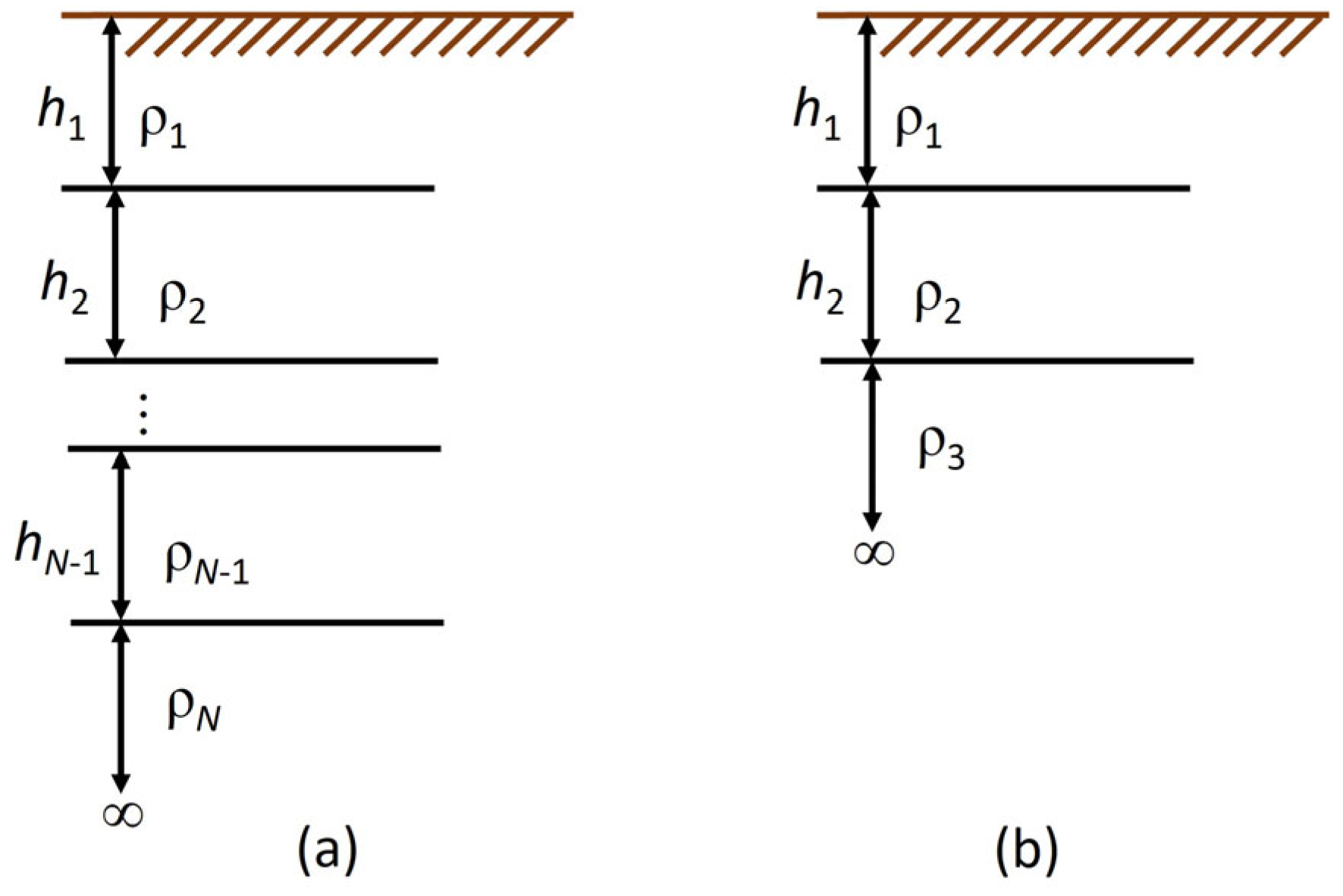
The results obtained with the Wenner method are only specific resistivities as a function of distance and do not provide information about the soil structure independently. They need to be linked to horizontally multi-layered analytical soil models developed in the past [15,16,17,18,19]. It is necessary to determine the parameters of analytical soil models so that the calculated resistivities fit the measured data best. An inverse problem is described, which can be solved successfully using optimization methods. N is the number of soil model layers, which can be two or more. In the rest of this article, a three-layered model is used, so Figure 2 shows a general N-layered and a three-layered soil model that was used.
Each soil layer has a specific soil resistance, marked from ρ1 to ρN, and a layer thickness marked from h1 to hN−1. The deepest, the Nth layer, has an infinite depth. The soil is homogeneous within a single layer. The analytic expression of apparent resistance depends on distance d (shown in Figure 1), and it is written in (3) [29].
ρ = ρ 1 1 + 2 d 0 f ( λ ) J 0 ( λ d ) J 0 ( 2 λ d ) d λ
ρ1 is the specific resistivity of the first layer, Jo is Bessel’s function of the first kind, and d is the distance between the electrodes. Equation (3) contains the function f(λ), which is calculated using (4).
f ( λ ) = α 1 ( λ ) - 1
α1 for the N-layered model is calculated with the sequence of equations written in (5).
K 1 ( λ ) = ρ 2 α 2 ( λ ) ρ 1 ρ 2 α 2 ( λ ) + ρ 1 ; α 1 ( λ ) = 1 + 2 K 1 e 2 λ h 1 1 K 1 e 2 λ h 1 K N 2 ( λ ) = ρ N 1 α N 1 ( λ ) ρ N 2 ρ N 1 α N 1 ( λ ) + ρ N 2 ; α N 2 ( λ ) = 1 + 2 K N 2 e 2 λ h N 2 1 K N 2 e 2 λ h N 2 K N 1 ( λ ) = ρ N ρ N 1 ρ N + ρ N 1 ; α N 1 ( λ ) = 1 + 2 K N 1 e 2 λ h N 1 1 K N 1 e 2 λ h N 1
In the continuation of the paper, a three-layered model is used and, based on (3) for the three-layered model, α1 is calculated with the equations presented in (6).
K 1 ( λ ) = ρ 2 α 2 ( λ ) ρ 1 ρ 2 α 2 ( λ ) + ρ 1 ; α 1 ( λ ) = 1 + 2 K 1 e 2 λ h 1 1 K 1 e 2 λ h 1 K 2 ( λ ) = ρ 3 ρ 2 ρ 3 + ρ 2 ; α 2 ( λ ) = 1 + 2 K 2 e 2 λ h 2 1 K 2 e 2 λ h 2
The calculation of ρ in (3) is used in the following as part of the objective function, and it is compared with the measured value. The expression f(λ) [J0d) − J0(2λd)] is a function of the distances d and soil properties (ρ and h). Since the accuracy of the calculation depends on the chosen values of the integration step, stopping criterion, etc., they are given briefly. Only numerical integration can be performed. The integrands oscillate, depending on λ, due to the content of the Bessel functions. The function inside the integral is negligibly small for sufficiently large λ [16]. Due to the oscillatory nature of the function, the integration is stopped when the value of the integrated function is successively 10 times smaller than 10−6. The step used for the numerical integration is 10−2.
The numerical integration time can vary from case to case. The time-consuming Bessel functions do not depend on the soil parameters; they only depend on the distances d. Therefore, the part [J0d) − J0(2λd)] can be calculated before starting the optimization process and stored into an array of values.

3. The Use of a Horizontally Layered Soil Model for Inhomogeneous Soil

3.1. Disadvantages of Horizontally Layered Soil Model

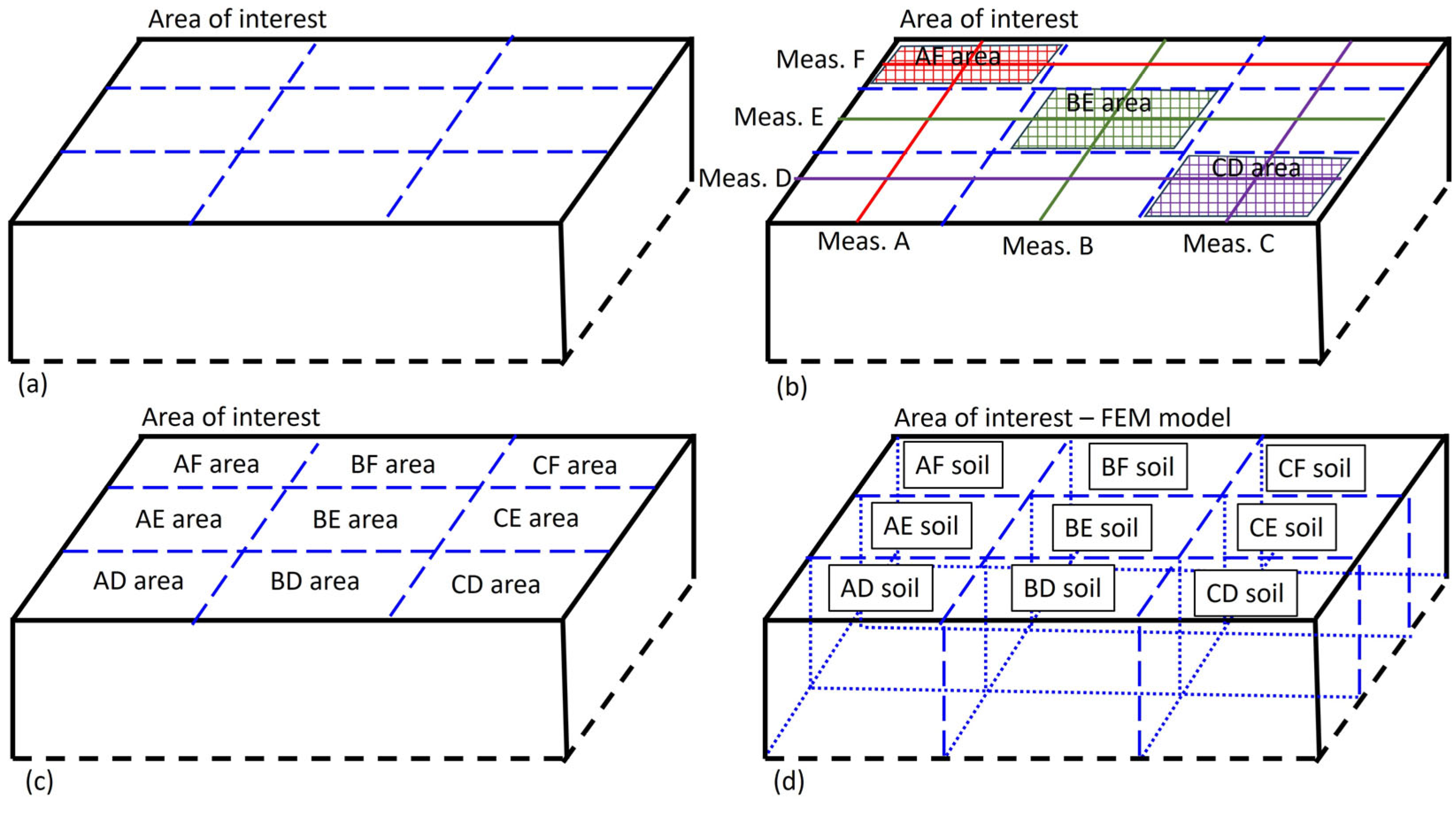
Using a horizontally layered soil model, it is assumed that the soil of the single soil layer is homogeneous. It is often unknown whether there is inhomogeneity in the soil. In the case of assuming inhomogeneity, measurements are required in several directions. Two possible approaches are shown in Figure 3.
The approach of using two or more directions of measurements is shown in Figure 3a. The average values of measurements are calculated for all directions and then are used in the whole area of interest. The disadvantage of this approach is that the soil resistivity is too low in some areas and, in some, too high. With that, the grounding system in the areas with excess resistivity is over-dimensioned, and in the areas with insufficient resistivity, it is dimensioned inadequately.
The approach of dividing the area into smaller parts is used in Figure 3b. In this case, the average values of measurements L3 and L4 are calculated and used in the area of crossing lines L3 and L4. The same approach is also used for the areas with lines L5 and L6, L7 and L8, and L9 and L10. The strong disadvantage of this approach is that the current does not flow deep into the soil, and, with that, the resistivity of deeper soil is not considered. We could increase the area of interest presented in Figure 3b and also extend lines L3–L10 beyond the field of interest; however, in many cases, in a real environment, it is not possible to make measurements outside the presented area of interest, due to factors such as buildings.

3.2. A New Approach with the Possibilty for Consideration of Inhomogeneity When Also Using a Horizontally Layered Model

We developed an approach in which we can consider the inhomogeneity of the soil, and, at the same time, take into account the deeper layers of the soil. It was assumed that measurements with the Wenner method can only be carried out within the area of interest due to the configuration of the environment.
The parameters’ determination process is shown in Figure 4.
The determination of the soil parameters can be explained in the following steps:
Step 1: The area of interest is divided into nine equal parts, as presented in Figure 4a.
Step 2: Measurements using Wenner’s method are made in the middle of the subareas. Measurements A, B, and C are made in one direction and measurements D, E, and F are made using the perpendicular direction, as shown in Figure 4b.
Step 3: Measurements that are crossing in the same subarea are used to determine the soil parameters. For example, measurements C and D are crossing in the lower right subarea, as can be seen in Figure 4b, and in Figure 4c, it is marked as a CD area. Based on the apparent resistivities of measurements C and D, the average apparent resistivities are calculated and marked with CD apparent resistivities, which are then used for determination of the parameters of the CD area. For each subarea, appropriate average apparent resistivities are calculated, as shown in Figure 4c.
Step 4: For each average apparent resistivity (AD, AE, AF, BD, BE, BF, CD, CE, and CF), soil parameters are determined using the analytical soil model and an appropriate optimization method.
Step 5: Based on the calculated soil parameters, a 3D FEM model is made, as presented in Figure 4d.

3.3. Test Model Using FEM

Usually, the soil structure is not known exactly, so for testing the approach described in Section 3.2, the model used was made by the FEM. We decided to use a three-layered analytical soil model because it is more accurate than a two-layered one, but, at the same time, it is easier to make an FEM model as in the case of a model with four or more layers. The three-layered model is not much less accurate than models with four or more layers.
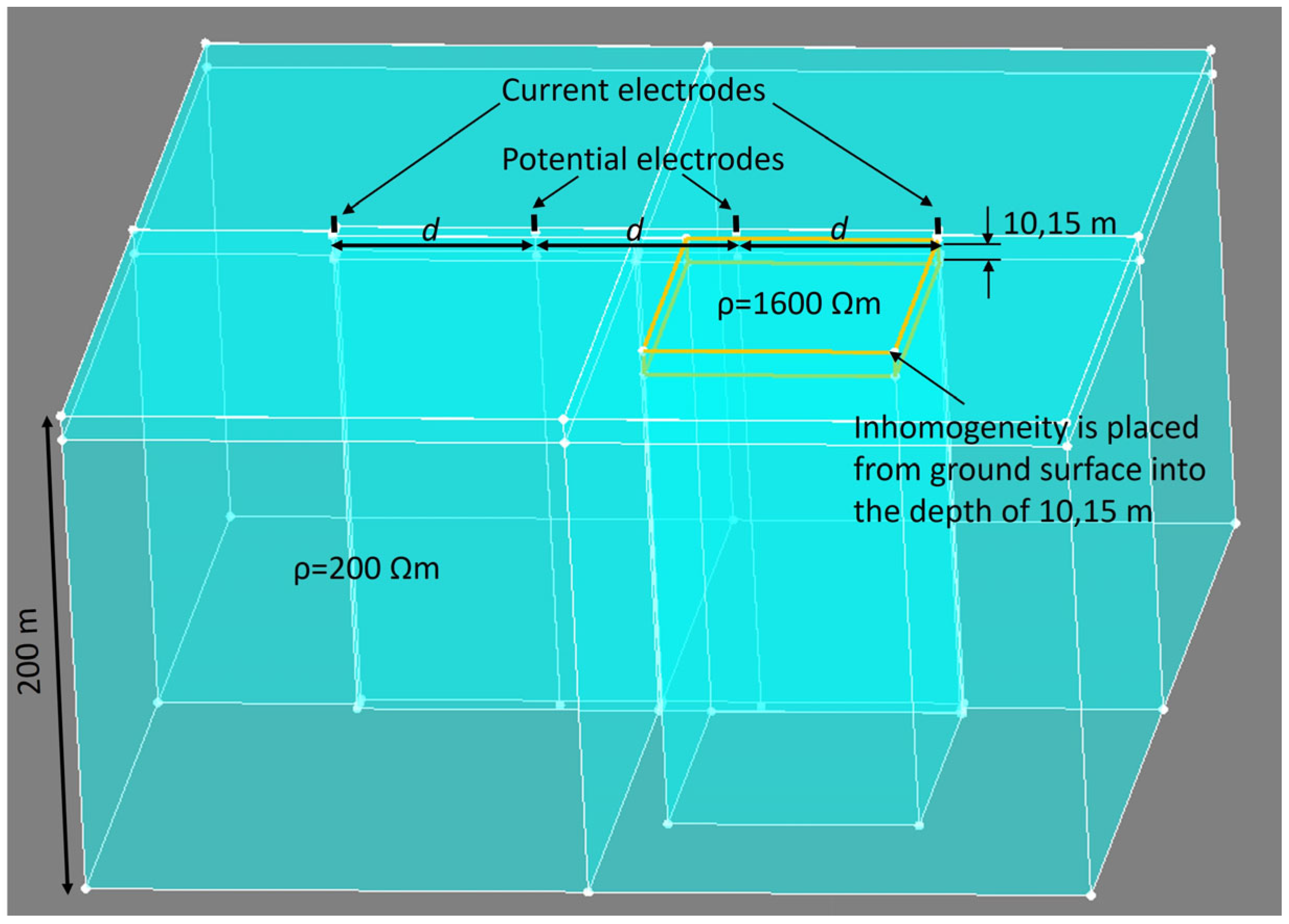
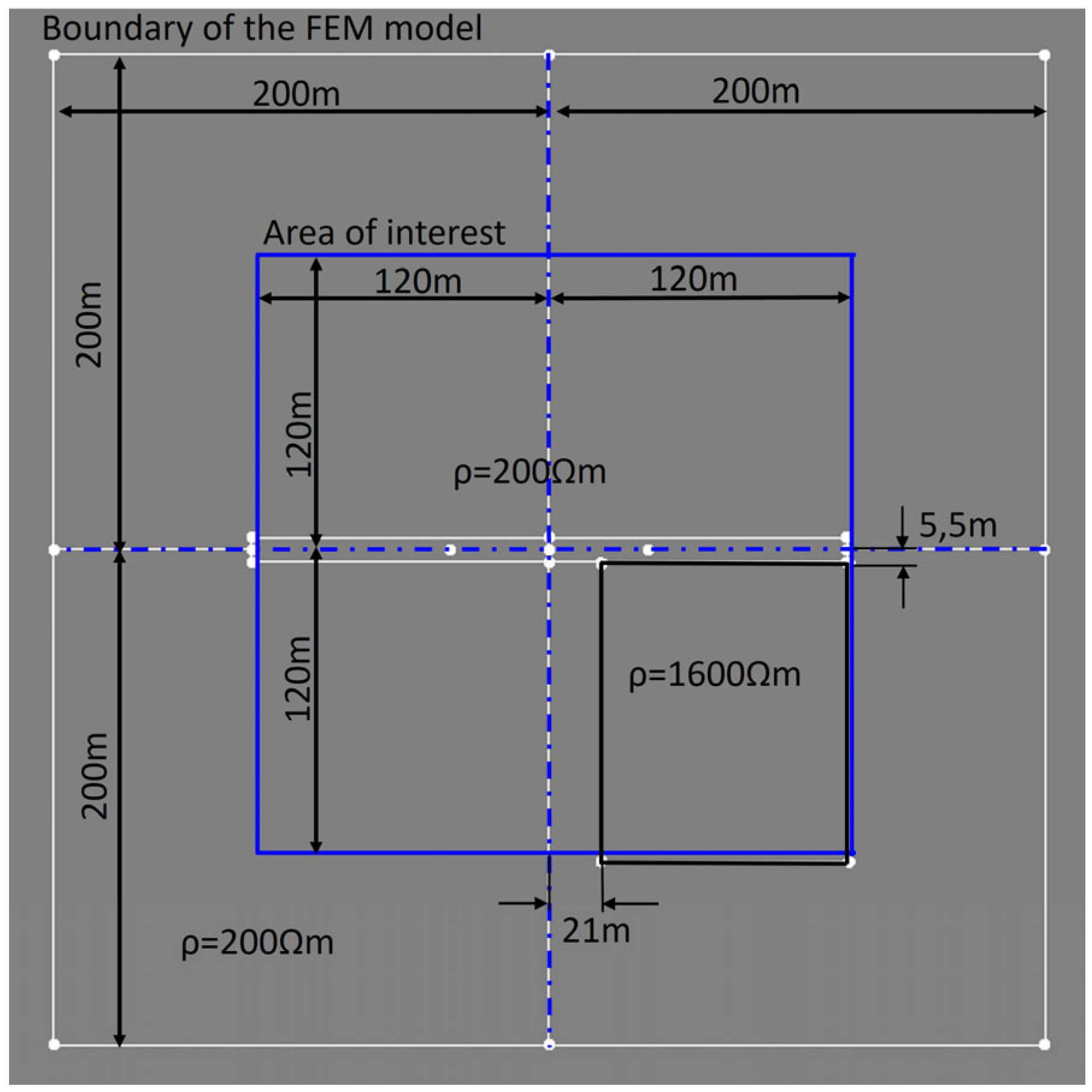
The 3D FEM model used for tests is presented in Figure 5, and the 2D cross-section on the surface of the ground is presented in Figure 6.
In Figure 6, it can be seen that the area of interest is smaller than the model. With that, the influence of the boundary conditions on the calculation results is eliminated. The position of the electrodes is given parametrically, allowing the distance d to change and thus simulate measurements with the Wenner method.
The FEM model is made using the Altair Flux 3D commercial software. The second-order differential equation (Equation (7)) is solved by the finite element method.
d i v σ g r a d V = 0
[σ] is the tensor of the conductivity of the medium and V is the electric potential.

4. Selected Optimization Methods

Using an analytical soil model, we searched for the soil data that fit the measured data best and, therefore, we solved an optimization problem. The parameters’ determination procedure must be repeated for each subarea shown in Figure 4c. Therefore, it is important that the selected optimization is suitable for the presented problem.
The objective function (OF) used for the determination of the soil parameters is written in (8).
f = 1 n i = 1 n ρ c _ i ρ m _ i ρ m _ i · 100 ( % ) ,
where ρc_i are the calculated apparent resistivity values based on the analytical soil model and ρm_i are the measured apparent resistivity values based on the Wenner method measurement. n is the number of different distances d that were used for the measurements. The term 1/n is included in the objective function to achieve comparability of results for measurements with different numbers of used distances d.
Various optimization methods can be used for determining soil parameters. In [20,22,29], standard optimization methods were used, and in [18,25,26,27,28], metaheuristics were used, as in the presented work. Metaheuristics are based on natural selection and the survival of the fittest, which makes them robust and not prone to becoming stuck in the local minima. Different optimization methods have different success rates for different optimization problems. In the past, a genetic algorithm [18,25,26,27] or differential evolution [28] was used for determining soil parameters, but different methods were not compared with each other. In the presented work, different metaheuristics are compared with each other using a three-layered soil model. The goal is to determine the most suitable among the selected ones for the presented problem.
We tested Differential Evolution [28,35,36,37,38,39,40,41,42,43,44,45,46] using three different strategies, namely DE/rand/1/exp, DE/rand/2/exp, and DE/best/1/bin. DE has two internal parameters, which are step size and the crossover probability constant. Based on our experiences using optimization methods, for all calculations, the step size (F) was set to 0.6 and the crossover probability (CR) was set to 0.8. The same step size and crossover probability were used in [43,44], where, similarly, the inverse problem was solved by finding the appropriate parameters of the magnetization curve in [43] and the DC engine parameters in [44], and the selected DE parameters were proven to be appropriate.
Teaching–Learning-Based Optimization (TLBO) [47,48,49,50,51,52,53,54,55,56,57] was also tested. The number of Objective Function Evaluations (OFEs) performed was determined as OFEs = (2 × population size × iterations). This approach of calculating OFEs was possible because the implementation was used with no duplication elimination phase. TLBO has no internal parameters.
Artificial Bee Colony (ABC) was also used, based on good previous experience [58,59,60,61,62]. It has three phases: foragers, onlookers, and scout. In the implementation, we used [61], and the number of OFEs was determined dynamically, as the scout phase is not proceeded for every iteration. Many practical problems were solved using the ABC method [63,64,65,66,67]. The internal parameter limit was set to 100, because such a setting of this parameter had achieved good results on similar problems.
For the sake of clarity, the basic equations of the optimization methods used are written down [68]. For different DE strategies, the variation is first determined by (9) for DE/rand/1/exp, by (10) for DE/rand/2/exp, and by (11) for DE/best/1/bin.
v i ( g ) = x r 1 ( g ) + F · x r 2 ( g ) x r 3 ( g )
v i ( g ) = x r 1 ( g ) + F · x r 2 ( g ) x r 3 ( g ) + F · x r 4 ( g ) x r 5 ( g )
v i ( g ) = x b e s t ( g ) + F · x r 2 ( g ) x r 3 ( g )
After that, crossover is performed according to (12).
u i ( g ) = v i , j ( g ) if r j C R or j = j r a n d x i , j ( g ) otherwise
The new population is obtained using the selection written by (13), which is made after crossover.
x i ( g + 1 ) = u i ( g ) if f u i ( g ) f x i ( g ) x i ( g ) otherwise
For the ABC method, a new candidate is generated by (14) (foragers phase).
v i j = x i j + ϕ i j · x i j x k j
Φij is a random number between −1 and 1 and ki. The foragers phase is followed by the onlooker phase, which represents the probability of selecting a solution, expressed by (15).
P i = f i j = 1 n f j
If a solution does not improve after a predefined number of iterations (limit), it is abandoned and replaced (abandonment and scout phase).
The TLBO method starts with the teacher phase, expressed by (16).
X n e w = X c u r r e n t + r · X t e a c h e r T F · X ¯
TF is the teaching factor, which is commonly 1 or 2, and r is a random number. The teaching phase is followed by the learning phase, expressed by (17).
X n e w = X i + r · X j X i if f X j < f X i X i + r · X i X j otherwise
The lowercase letters x, v, and u represent the individual members of the population, while the uppercase X represents a population vector.
The analysis in the remainder of this article is based on the use of the three-layered model, whose parameters are shown in Figure 2b. The limits of specific resistivity of the soil are set between the lowest resistivity of wet, well-conducting soil (5 Ωm) and the highest specific resistivity of stony ground (3500 Ωm). In the Wenner method, the current only penetrates to a certain depth, so it makes sense to define layers only to a certain depth. The parameters’ limits are shown in Table 1.
All five metaheuristics, DE/rand/1/exp, DE/rand/2/exp, DE/best/1/bin, ABC, and TLBO, were tested under the same conditions, and the tests were performed following the guidelines presented in [69]. We used 18,000 OFEs as the stopping criteria. In the case of ABC, we also counted scouts, and in the case of TLBO, we considered both phases of the algorithm, the Teaching and Learning phases. Six times the number of the parameters was used for the population number (NP). The parameters for different optimization methods are presented in Table 2.
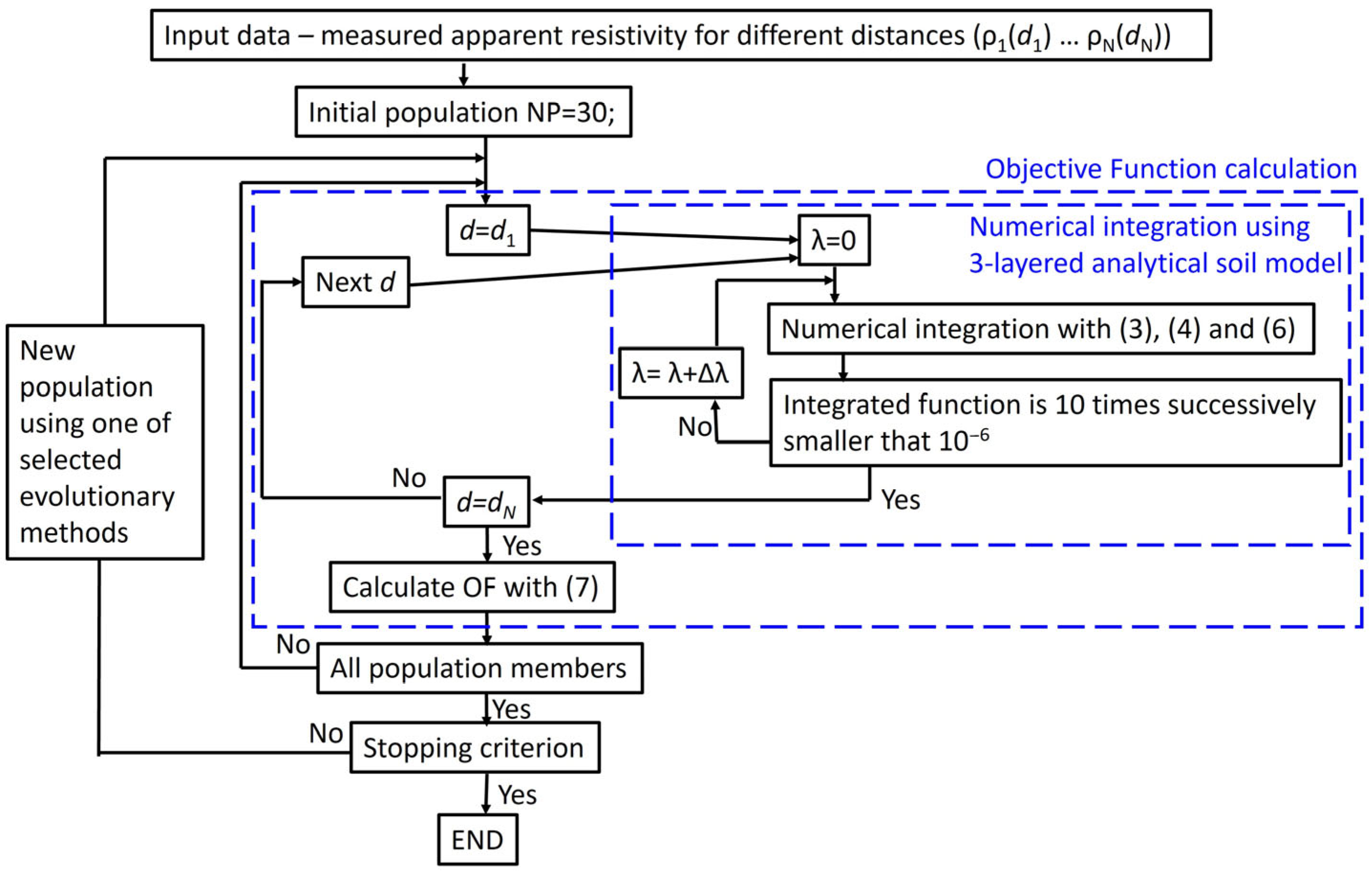
The algorithm of the calculation procedure considering the presented problem is shown in Figure 7.
Numerical integration is the most time-consuming part of the algorithm presented in Figure 7. As it is necessary to repeat the soil parameters’ determination procedure for nine subareas, it would be advantageous if the calculation time were as short as possible.

5. Results Using Test Data Obtained with FEM Model

Using the FEM model presented in Section 3.3, Wenner’s measuring method was simulated for lines A, B, C, D, E, and F, as presented in Figure 4b. The values of the apparent resistivity are shown in Table 3 (the measurement simulation was performed according to Step 2 in Section 3.2).
According to Step 3 in Section 3.2., the average apparent resistivity was calculated for measurements which were crossing in some subarea. The average values for the nine subareas presented in Figure 4c are shown in Table 4.
Table 5, Table 6, Table 7, Table 8, Table 9, Table 10, Table 11, Table 12 and Table 13 present the calculation results for each subarea (AD, AE, AF, BD, BE, BF, CD, CE, and CF) separately. Each table contains the OF’s best value (B), worst value (W), mean value (M), and Standard Deviation (SD) for all five optimization methods used. The calculated parameters of the best solution are also presented in the tables for each optimization method used.
For easier conclusions, the mean OF values for all five optimization methods and all nine subareas are shown in Figure 8.
Based on Table 5, Table 6, Table 7, Table 8, Table 9, Table 10, Table 11, Table 12 and Table 13 and Figure 8, the following can be seen:
  • ABC was better than other methods in the case of seven subareas (AD, AE, AF, BD, CD, CE, and CF).
  • In the case of BE, DE/rand/2/exp and TLBO were slightly better than ABC.
  • In the case of BF, DE/rand/1/exp and DE/rand/2/exp were slightly better than ABC.
  • In the case of the CD subarea, ABC was 19% better than the next best.
  • In the case of the CE subarea, ABC was 23% better than the next best.
  • In the case of the CF subarea, ABC was 25% better than the next best.
Taking into account the given findings, we can claim that the ABC method is the best among the tested methods for the problem considered.
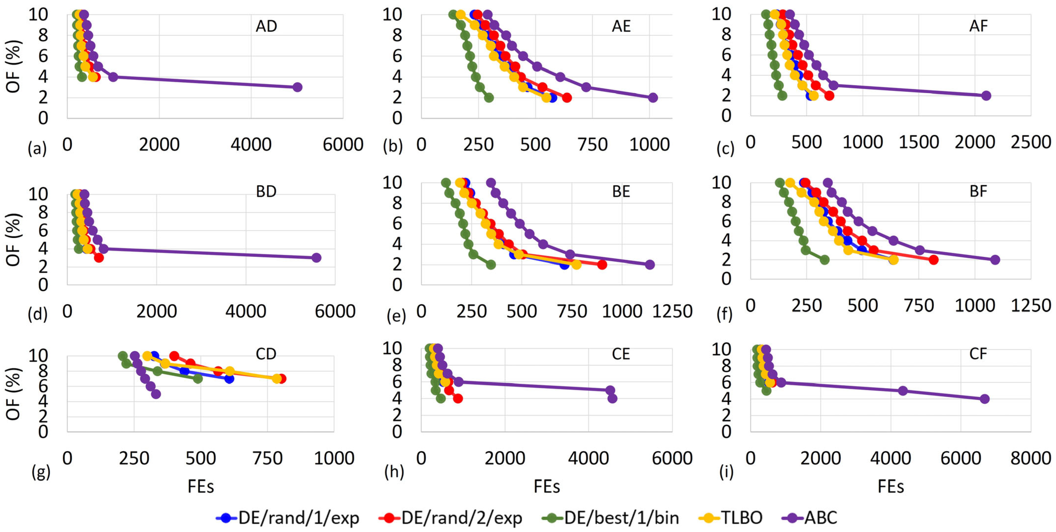
When comparing evolutionary methods, the convergence of each method is also important. Due to the use of the random generator, each calculation flow is different. Therefore, the average convergence speed of each method was determined. The results are shown in Figure 9, where the average FEs required to achieve OF < 10%, OF < 9%, etc., with the OF values shown.
Based on Figure 8, it can be seen that the convergence of DE/best/1/bin was fastest. The convergences of DE/rand/1/exp, DE/rand/2/exp, and TLBO were similar. The convergence of ABC was fastest in the case of CD and slowest for all the other cases. It is interesting that ABC gave the best results despite the slowest convergence.
As mentioned, the calculation time is also an important calculation parameter, due to the nine subareas. The mean calculation times for 50 independent runs for the five optimization methods and all nine subareas are presented in Table 14.
Based on Table 14, it can be seen that the calculation times of the ABC method are longer than those of the other methods. The different calculation times are due to the different search spaces in the cases of different methods. The time of numerical integration of expression (3) depends on the soil parameters during the optimization, which leads to the searched soil parameters.

5.1. The Use of Memory Assistance

Although ABC was the best among the tested methods, the calculation times using ABC were longer than the calculation times using other methods. Although the pre-calculation of time-consuming Bessel functions was used (Section 2.2), it will be useful to shorten the calculation time. We used Memory Assistance [70].
We used two different Memory Assistances:
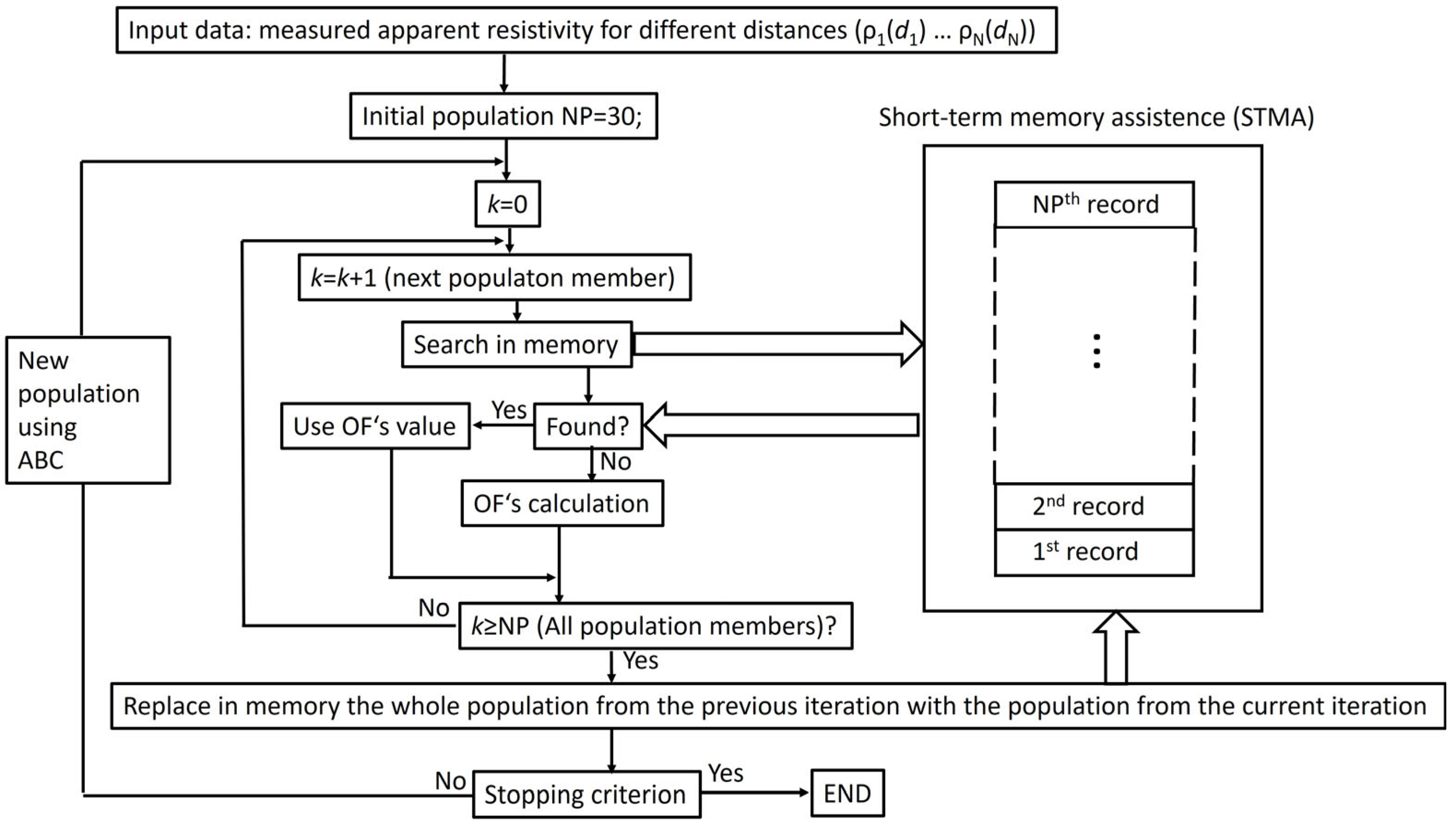
  • Short-Term Memory Assistance (STMA): After each iteration, the whole population is saved into memory, and, in each iteration, the population members are compared with members from only one previous iteration. In this approach, only memory is used for one population set. In the presented case, this is ((5 parameters + OF) × 30 population members) memory locations.
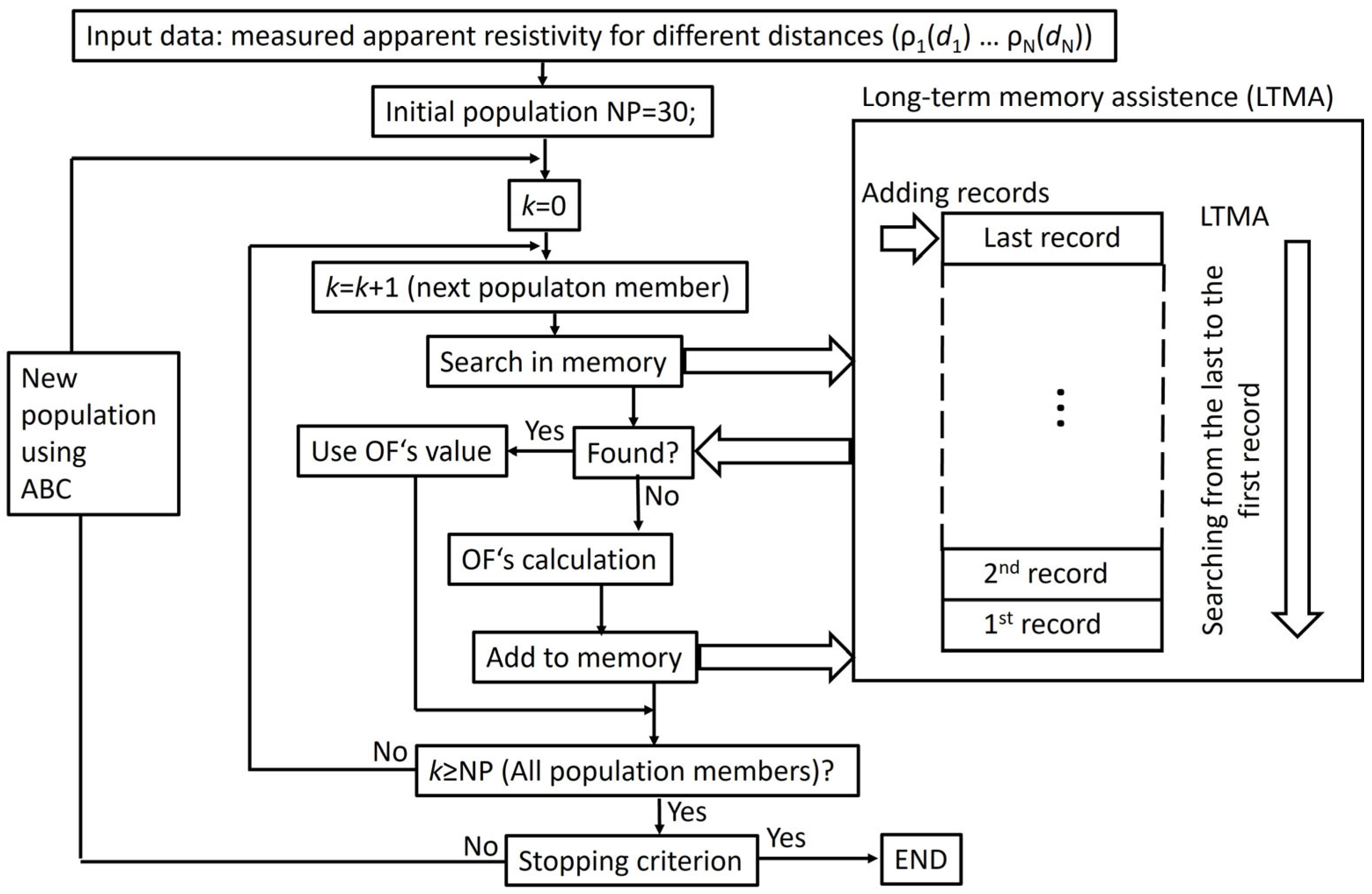
  • Long-Term Memory Assistance (LTMA): Each population member is compared with all the members written into memory, obtained from all the previous iterations. If the calculated member is not found in the memory, it is added to the memory. The search in the memory starts from the last added to the first added. When the same population member is found, the search is finished. Theoretically, ((5 parameters + OF) × 30 population members × 600 iterations) locations of memory can be used.
The STMA algorithm is presented in Figure 10 and the LTMA algorithm is shown in Figure 11.
The expression “record” used in Figure 10 and Figure 11 means one set of parameters + OF’s values (ρ1, h1, ρ2, h2, ρ3, OF). An appropriate precision must be set, as these are differences in the parameters for which duplication may be identified. These values depend on the physical background of the problem, and they determine the decimal accuracy of the calculated parameters. The precisions used for the identification of duplications are presented in Table 15.
The results presenting the calculation times for ABC, ABC + STMA, ABC + LTMA, deviations of calculation times, and number of duplications for 50 independent runs for each subarea are presented in Table 16.
From Table 16, it can be seen that with the use of Memory Assistance, the calculation time was shortened by 21% in both cases, using STMA and LTMS. Although the mean number of duplications in the case of LTMA was 2643, which is higher than 1682 in the case of STMA, the memory handling time was longer in the case of LTMA compared to STMA. The advantage of STMA is its much lower use of memory space, and, accordingly, it can be concluded that STMA is a better choice for the presented problem.
It is important to emphasize that the use of Memory Assistance is not required; it is just a suggestion if we want to reduce the time of soil parameters’ determination.

5.2. Test of Four-, Five-, and Six-Layered Soil Models

Although the three-layered model is easier for FEM modeling, we also conducted tests with four-, five-, and six-layered models to determine whether these models were better. For all nine subareas, four-, five-, and six-layered models were used for determining soil parameters. The calculated best OF (B), worst OF (W), mean OF (M), and Standard Deviation (SD) are presented in Table 17, where the results of the three-layered model copied from Table 5, Table 6, Table 7, Table 8, Table 9, Table 10, Table 11, Table 12 and Table 13 are also presented, which offers an easier comparison of the results.
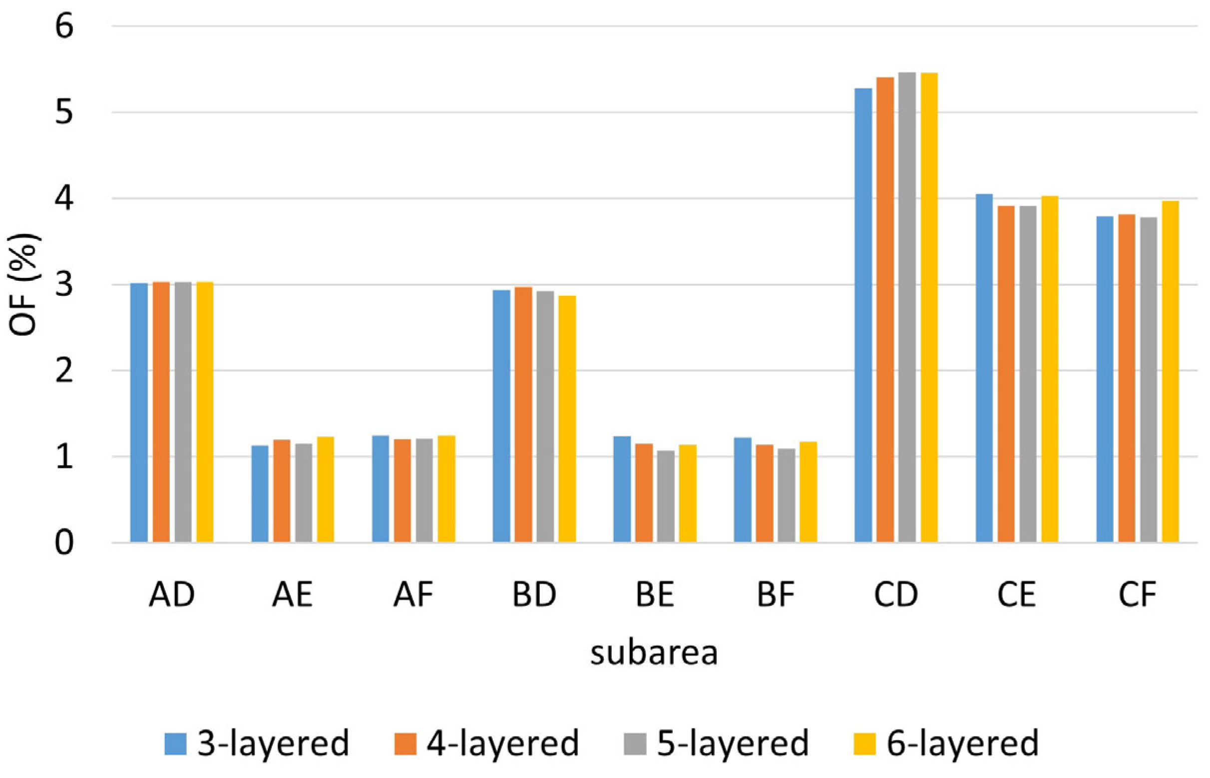
For easier evaluation of the differences between the soil models, the mean OF values for all subareas and all soil models are presented in Figure 12.
Based on Figure 12, it can be seen that there were no significant differences between mean OF values using models with different layers. In the case of AD and CD, the lowest mean OF was obtained using the three-layered model. Based on this, it can be concluded that the three-layered model is appropriate, especially if we consider that FEM modeling is easier using a lower number of soil layers.

5.3. Verification of Results

For verification of the results, an FEM model was made, based on the soil determination procedure presented in Section 3.2.
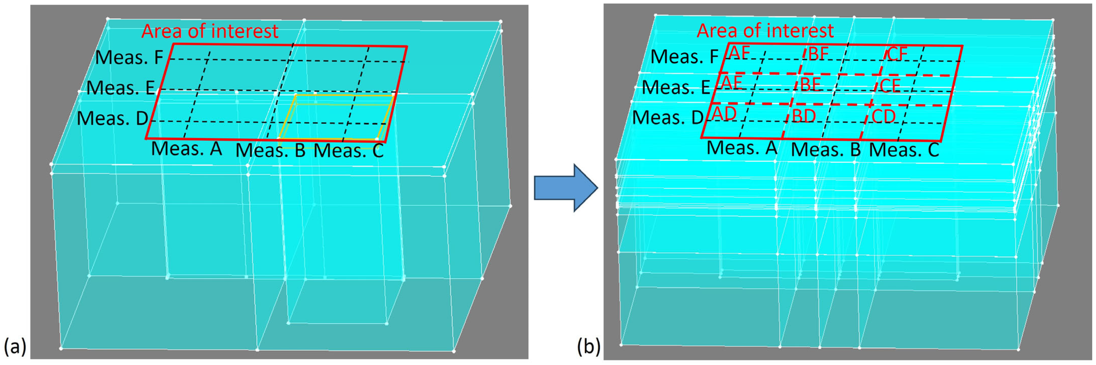
The basic model, together with the determined model, is presented in Figure 13.
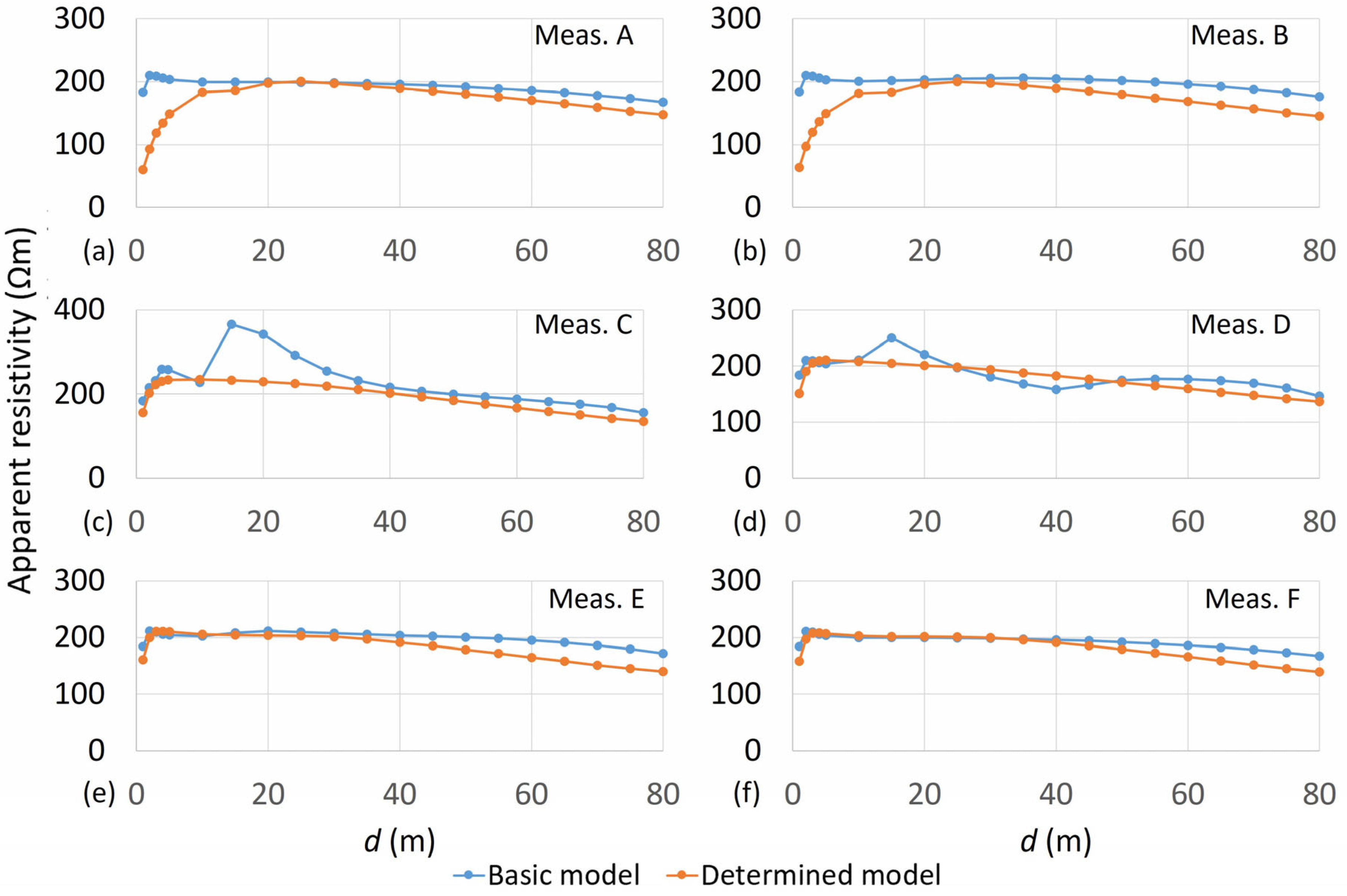
The basic model (Figure 13a) is presented in detail in Figure 5. The determined FEM model presented in Figure 13b was obtained after the soil-determined procedure. The soil parameters in each subarea were calculated using the ABC method and are presented in Table 5, Table 6, Table 7, Table 8, Table 9, Table 10, Table 11, Table 12 and Table 13. In both FEM models, the Wenner measurement was simulated at the lines marked Meas. A to Meas. F, which are presented in Figure 13a,b. The differences were determined using the expression for OF written in (8). The obtained differences were as follows: 16.1% for Meas. A, 18.9% for Meas. B, 13.1% for Meas. C, 19.1% for Meas. D, 8.5% for Meas. E, and 6.2% for Meas. F. Although the differences were up to 19%, it should be noted that the mean OF calculated for different subareas (Table 5, Table 6, Table 7, Table 8, Table 9, Table 10, Table 11, Table 12 and Table 13) was also over 6%. To show that the presented differences are acceptable, the apparent resistivity for the Basic and Determined models at lines Meas. A to Meas. F is presented in Figure 14.
From Figure 14, the comparability between the apparent resistivity obtained from the basic model and apparent resistivity obtained from the determined model can be seen. Based on this, the accuracy of the suggested method for soil modeling can be confirmed in the case of inhomogeneities.
The test calculations were made with a cube, but, in reality, strange forms of geological anomalies can occur in the ground, as shown in Figure 15a.
The geological anomaly influences the Wenner measurement, which is performed on the lines above it, as shown in Figure 15a. Based on the Wenner measurements, an FEM model of the soil was created consisting of nine regions, each of which is defined by a different three-layer soil model, as shown in Figure 15b. In this approach, any anomaly that affects the Wenner measurement is captured.

6. Conclusions

This paper introduces an approach that describes the use of an analytical horizontally layered soil model for inhomogeneous soil. In this approach, deeper layers of the soil were also considered, which was enabled using higher distances d in the Wenner method, as in case of simple division of the area into smaller parts. The presented approach is unique and was not found in the literature. Since the soil structure is usually unknown, FEM models were used for presentation and verification of the presented approach. In Section 5.3, the validation of the approach is presented, which confirms its accuracy.
As described in Section 3.2, the soil determination procedure using an optimization method should be performed for nine subareas. Due to this fact, it is important to select an appropriate optimization method that works well for the presented problem. Among the tested methods, which were DE/rand/1/exp, DE/rand/2/exp, DE/best/1/bin, TLBO, and ABC, ABC was best, reaching the lowest mean OF value for seven out of the nine subareas. Although the convergence of ABC was not the fastest, it was able to achieve the best results. Therefore, ABC can be suggested as the best method for the presented problem.
As mentioned in Section 5, the different calculation times were due to the different search space in the case of different methods. The time of the integration of (3) depended on the soil parameters. The disadvantage of ABC was the longer calculation time, but the problem with the faster methods was that they were not as successful as ABC. Although the pre-calculation of time-consuming Bessel functions was used (Section 2.2), the calculation times were still long. The STMA and LTMA approaches are presented in this paper. With both of them, the calculation time using a precision of 0.1 mΩm for apparent resistivity and 0.1 mm for soil layer depth (Section 5.1) could be shortened by 21%. The STMA approach, which uses much less memory space than LTMA, can be suggested as the better choice.
The selected soil model was a three-layered model because it is easier to make an FEM model using a three-layered model than to use a four-, five-, or six-layered model. Although the three-layered model was selected, in Section 5.2, four-, five-, and six-layered models were also tested to confirm the correct selection. It was confirmed that no other model was significantly better than the three-layered one. In two of the nine subareas, the lowest mean OF was obtained using the three-layered model.
Finally, we could conclude that all the elements needed for determining soil parameters are described in the presented work, which is a new approach using a horizontally layered analytical soil model for inhomogeneous soil. The appropriate evolutionary optimization method and the appropriate soil model were selected, and Memory Assistance was also used. It should also be mentioned that the approach using FEM models for simulation of Wenner’s method measurements, which was not found in the literature, offers good possibilities for analyses, due to the fact that the soil used in the FEM model is known, which is not the case for real ground.
The FEM approach is the most universal, but it involves complex modeling. It allows the definition of different layers in different areas of the problem, defining inhomogeneities, etc. Dimensioning is significantly faster with programs that are intended for dimensioning grounding systems, and they usually already have a library of grounding elements. For example, XGSLab is based on the partial element equivalent method (PEEM) and only allows multi-layer horizontal soil models, so inhomogeneities in the soil cannot be captured. Alternatively, WinIGS allows the electrical power system to be connected with the grounding system but only allows a two-layer horizontal soil model.
In the future, the findings about the soil models and the evolutionary methods presented in this paper will be used to solve optimization problems in electromagnetics.

Author Contributions

Conceptualization, M.J.; methodology, M.J. and M.T.; software, M.J.; validation, M.T. and M.J.; formal analysis, M.J. and M.T.; investigation, M.J. and M.T.; writing—original draft preparation, M.J.; writing—review and editing, M.J. and M.T.; supervision, M.J.; project administration, M.J.; funding acquisition, M.J. All authors have read and agreed to the published version of the manuscript.

Funding

This research was funded by the Slovenian Research and Innovation Agency, grant number P2-0114, and the APC was funded by the Slovenian Research and Innovation Agency.

Institutional Review Board Statement

Not applicable.

Informed Consent Statement

Not applicable.

Data Availability Statement

The data presented in this study are available in this article and on request from the corresponding author. The data are not publicly available due to the use of the laboratory equipment.

Conflicts of Interest

The authors declare no conflicts of interest.

References

  1. Zhu, L.; Jiang, H.; Yang, F.; Luo, H.; Li, W.; Han, J. FEM Analysis and Sensor-Based Measurement Scheme of Current Distribution for Grounding Electrode. Appl. Sci. 2020, 10, 8151. [Google Scholar] [CrossRef]
  2. Zeng, Z.; Udpa, L.; Udpa, S.S. Finite-Element Model for Simulation of Ferrite-Core Eddy-Current Probe. IEEE Trans. Magn. 2012, 46, 905–909. [Google Scholar] [CrossRef]
  3. Egea, A.; Almandoz, G.; Poza, J.; Ugalde, G.; Escalada, A.J. Axial-Flux-Machine Modeling with the Combination of FEM-2-D an Analytical Tools. IEEE Trans. Ind. Appl. 2012, 48, 1318–1326. [Google Scholar] [CrossRef]
  4. Fu, W.N.; Ho, S.L.; Zhou, P. Reduction of Computing Time for Steady-State Solutions of Magnetic Field and Circuit Coupled Problems Using Time-Domain Finite-Element Method. IEEE Trans. Magn. 2012, 48, 3363–3366. [Google Scholar] [CrossRef]
  5. Wang, G.; Wang, S.; Duan, N.; Huangfu, Y.; Zhang, H.; Xu, W.; Qiu, J. Extended Finite-Element Method for Electric Field Analysis of Insulating Plate with Crack. IEEE Trans. Magn. 2015, 51, 7205904. [Google Scholar]
  6. Trlep, M.; Hamler, A.; Jesenik, M.; Štumberger, B. The FEM-BEM Analysis of Complex Grounding Systems. IEEE Trans. Magn. 2003, 39, 1155–1158. [Google Scholar] [CrossRef]
  7. Bruckner, F.; Vogler, C.; Feisch, M.; Praetorius, D.; Bergmair, B.; Hubner, T.; Fuger, M.; Suess, D. 3D FEM–BEM-coupling method to solve magnetostatic Maxwell equations. J. Magn. Magn. Mater. 2012, 324, 1862–1866. [Google Scholar] [CrossRef]
  8. Salas, R.A.; Pleite, J.; Olias, E.; Baarado, A. Theoretical–experimental comparison of a modeling procedure for magnetic components using finite element analysis and a circuit simulator. J. Magn. Magn. Mater. 2008, 320, 1024–1028. [Google Scholar] [CrossRef]
  9. Kurose, H.; Ohtake, M.; Miyagi, D.; Takahashi, N. 3-D FEM analysis of thermal degradation in writing and reading characteristics of a perpendicular magnetic head. J. Magn. Magn. Mater. 2008, 320, 2917–2920. [Google Scholar] [CrossRef]
  10. Zona, A.; Ranzi, G. Finite element models for nonlinear analysis of steel–concrete composite beams with partial interaction in combined bending and shear. Finite Elem. Anal. Des. 2011, 47, 98–118. [Google Scholar] [CrossRef]
  11. Melenk, J.M.; Babuška, J. The partition of unity finite element method: Basic theory and applications. Comput. Methods Appl. Mech. Eng. 1996, 139, 289–314. [Google Scholar] [CrossRef]
  12. Hansbo, A.; Hansbo, P. A finite element method for the simulation of strong and weak discontinuities in solid mechanics. Comput. Methods Appl. Mech. Eng. 2004, 193, 3523–3540. [Google Scholar] [CrossRef]
  13. Robles, K.P.V.; Yee, J.-J.; Kee, S.-H. Effect of the Geometrical Constraints to the Wenner Fout-Point Electrical Resistivity Test of Reinforced Concrete Stabs. Sensors 2021, 21, 4622. [Google Scholar] [CrossRef]
  14. Chik, Z.; Islam, T. Near Surface Soil Characterizations Through Soil Apparent Resistivity: A Case Study. In Proceedings of the 7th International Conference on Intelligent Data Acquisition and Advanced Computing System: Technology and Applications, Berlin, Germany, 12–14 September 2013; pp. 57–60. [Google Scholar]
  15. Southey, R.D.; Siahrang, M.; Fortin, S.; Dawalibi, F.P. Using Fall-of-Potential Measurements to Improve Deep Soil Resistivity Estimates. IEEE Trans. Ind. Appl. 2015, 51, 5023–5029. [Google Scholar] [CrossRef]
  16. Yang, H.; Yuan, J.; Zong, W. Determination of Three-Layer Earth Model from Wenner Four-Probe Test Data. IEEE Trans. Magn. 2001, 37, 3684–3687. [Google Scholar] [CrossRef]
  17. Karnas, G.; Maslowski, G.; Ziemba, R.; Wyderka, S. Influence of Different Multilayer Soil Models on Grounding System Resistance. In Proceedings of the International Conference on Lightning Protection ICLP, Vienna, Austria, 2–7 September 2012; pp. 1–4. [Google Scholar]
  18. Gonos, I.F.; Stathopulos, I.A. Estimation of Multilayer Soil Parameters Using Genetic Algorithms. IEEE Trans. Power Deliv. 2005, 20, 100–106. [Google Scholar] [CrossRef]
  19. Dawalibi, F.P.; Ma, J.; Southey, R.D. Behaviour of grounding systems in multilayer soils: A parametric analysis. IEEE Trans. Power Deliv. 1994, 9, 334–342. [Google Scholar] [CrossRef]
  20. Del Alamo, J.L. A Comparion among Eight Different Techniques to Achieve an Optimum Estimation of Electrical Grounding Parameters in Two-Layer Earth. IEEE Trans. Power Deliv. 1993, 8, 1890–1899. [Google Scholar] [CrossRef]
  21. Del Alamo, J.L. A second Order Gradient Technique for an Improved Estimation of Soil Parameters in a Two-Layer Earth. IEEE Trans. Power Deliv. 1991, 6, 1166–1170. [Google Scholar] [CrossRef]
  22. Lagace, P.J.; Fortin, J.; Crainic, E.D. Interpretation of Resistivity Sounding Measurements in N-Layer Soil using Electrostatic Images. IEEE Trans. Power Deliv. 1996, 11, 1349–1354. [Google Scholar] [CrossRef]
  23. Fakhraei, M.; Mahmoudian, M.; Rodrigues, E.M.G. Grounding System Modeling and Evaluation Using Integrated Circuit Based Fast Relaxed Vector Fitting Approach, Considering Soil Ionization. Appl. Sci. 2020, 10, 5632. [Google Scholar] [CrossRef]
  24. Perng, J.-W.; Kuo, Y.-C.; Lu, S.-P. Grounding System Cost Analysis Using Optimization Algorithms. Energies 2018, 11, 3484. [Google Scholar] [CrossRef]
  25. Calixto, W.P.; Neto, L.M.; Wu, M.; Yamanaka, K.; Moreira, E. Parameters Estimation of Horizontal Multilayer Soil Using Genetic Algorithm. IEEE Trans. Power Deliv. 2010, 25, 1250–1257. [Google Scholar] [CrossRef]
  26. Mohamed Nor, N.; Rajab, R.; Ramar, K. Validation of the Calculation and Measurement Techniques of Earth Resistance Values. Am. J. Appl. Sci. 2008, 5, 1313–1317. [Google Scholar]
  27. Zhiqiang, H.; Bin, Z. Soil Model’s Inversion Calculation Base on Genetic Algorithm. In Proceedings of the 7th Asia-Pacific International Conference on Lightning, Chengdu, China, 1–4 November 2011; pp. 225–230. [Google Scholar]
  28. Pereira, W.R.; Soares, M.G.; Nato, L.M. Horizontal Multilayer Soil Parameter Estimation Through Differential Evolution. IEEE Trans. Power Deliv. 2016, 31, 622–629. [Google Scholar] [CrossRef]
  29. Zhang, B.; Cui, X.; Li, L.; He, J. Parameter Estimation of Horizontal Multilayer Earth by Complex Image Method. IEEE Trans. Power Deliv. 2005, 20, 1394–1401. [Google Scholar] [CrossRef]
  30. Lagace, P.J.; Vuong, M.H. Graphical User Interface for Interpreting and Validating Soil Resistivity Measurements. In Proceedings of the IEEE ISIE (International Symposium on Industrial Electronics), Montreal, QC, Canada, 9–13 July 2006; pp. 1841–1845. [Google Scholar]
  31. Zou, J.; He, J.L.; Zeng, R.; Sun, M.W.; Yu, G.; Chen, S.M. Two-Stage Algorithm for Inverting Structure Parameters of the Horizontal Multilayer Soil. IEEE Trans. Magn. 2004, 40, 1136–1139. [Google Scholar] [CrossRef]
  32. Kang, M.J.; Boo, C.J.; Kim, H.C.; Zurada, J.M. A Nonlinear Regression based Approach for Multilayer Soil Parameter Estimation. Int. J. Control Autom. 2014, 7, 65–74. [Google Scholar] [CrossRef]
  33. IEEE Power and Energy Society. IEEE Guide for Measuring Earth Resistivity, Ground Impedance, and Earth Surface Potentials of Grounding Systems; The Institute of Electrical and Electronics Engineers, Inc.: New York, NY, USA, 2012. [Google Scholar]
  34. Barič, T.; Šljivac, D.; Stojkov, M. Validity limits of the expression for measuring soil resistivity by the Wenner method according to IEEE Standard 81-1983. Energija 2007, 56, 730–753. [Google Scholar] [CrossRef]
  35. Veček, N.; Črepinšek, M.; Mernik, M. On the influence of the number of algorithms, problems, and independent runs in the comparison of evolutionary algorithms. Appl. Soft Comput. 2017, 54, 23–45. [Google Scholar] [CrossRef]
  36. Veček, N.; Mernik, M.; Črepinšek, M. A chess rating system for evolutionary algorithms: A new method for the comparison and ranking of evolutionary algorithms. Inf. Sci. 2014, 277, 656–679. [Google Scholar] [CrossRef]
  37. Mallipeddi, R.; Suganthan, P.N.; Pan, Q.K.; Tasgetiren, M.F. Differential evolution algorithm with ensemble of parameters and mutation strategies. Appl. Soft Comput. 2011, 11, 1679–1696. [Google Scholar] [CrossRef]
  38. Das, S.; Suganthan, P.N. Differential Evolution: A Survey of the State-of-the-Art. IEEE Trans. Evol. Comput. 2011, 15, 4–31. [Google Scholar] [CrossRef]
  39. Saruhan, H. Differential evolution and simulated annealing algorithms for mechanical systems design. Eng. Sci. Technol. Int. J. 2014, 17, 131–136. [Google Scholar] [CrossRef]
  40. Mokan, M.; Sharma, K.; Sharma, H.; Verma, C. Gbest guided differential evolution. In Proceedings of the 9th International Conference on Industrial and Information Systems, Gwalior, India, 15–17 December 2014; pp. 1–6. [Google Scholar]
  41. Chattopadhyay, S.; Sanyal, S.K. Optimization of Control Parameters of Differential Evolution Technique for the Design of FIR Pulse-shaping Filter in QPSK Modulated System. J. Commun. 2011, 6, 558–570. [Google Scholar] [CrossRef]
  42. He, R.J.; Yang, Z.Y. Differential evolution with adaptive mutation and parameter control using Levy probability distribution. J. Comput. Sci. Technol. 2012, 27, 1035–1055. [Google Scholar] [CrossRef]
  43. Jesenik, M.; Beković, M.; Hamler, A.; Trlep, M. Analytical modelling of a magnetization curve obtained by the measurements of magnetic materials’ properties using evolutionary algorithms. Appl. Soft Comput. 2017, 52, 387–408. [Google Scholar] [CrossRef]
  44. Jesenik, M.; Ravber, M.; Trbušić, M. Innovative Approach for the Determination of a DC Motor’s and Drive’s Parameters Using Evolutionary Methods and Different Measured Current and Angular Speed Responses. Mathematics 2024, 12, 42. [Google Scholar] [CrossRef]
  45. Saad, A.; Engelbrecht, A.P.; Khan, S.A. An Analysis of Differential Evolution Population Size. Appl. Sci. 2024, 14, 9976. [Google Scholar] [CrossRef]
  46. Wang, X.; Yu, X. Differential Evolution Algorithm with Three Mutation Operators for Global Optimization. Mathematics 2024, 12, 2311. [Google Scholar] [CrossRef]
  47. Rao, R.V.; Savsani, V.J.; Vakharia, D.P. Teaching-learning-based optimization: A novel method for constrained mechanical design optimization problems. Comput. Aided Des. 2011, 43, 303–315. [Google Scholar] [CrossRef]
  48. Rao, R.V.; Savsani, V.J.; Vakharia, D.P. Teaching-Learning-Based Optimization: An optimization method for continuous non-linear large scale problems. Inf. Sci. 2012, 183, 1–15. [Google Scholar] [CrossRef]
  49. Rao, R.V.; Patel, V. An elitist teaching-learning-based optimization algorithm for solving complex constrained optimization problems. Int. J. Ind. Eng. Comput. 2012, 3, 535–560. [Google Scholar] [CrossRef]
  50. Črepinšek, M.; Liu, S.-H.; Mernik, L. A note on Teaching-learning-based optimization algorithm. Inf. Sci. 2012, 212, 79–93. [Google Scholar] [CrossRef]
  51. Waghmare, G. Comments on “A note on teachnig-learning-based optimization algorithm”. Inf. Sci. 2013, 229, 159–169. [Google Scholar] [CrossRef]
  52. Črepinšek, M.; Liu, S.-H.; Mernik, L.; Mernik, M. Is a comparison of results meaningful from the inexact replications of computational experiments. Soft Comput. 2016, 20, 223–235. [Google Scholar] [CrossRef]
  53. Shao, W.; Pi, D.; Shao, Z. A hybrid discrete optimization algorithm based on teaching-probabilistic learning mechanism for no-wait flow shop scheduling. Knowl.-Based Syst. 2016, 107, 219–234. [Google Scholar] [CrossRef]
  54. Sahu, B.K.; Pati, S.; Mohanty, P.K.; Panda, S. Teaching-learning based optimization algorithm based fuzzy-PID controller for automatic generation control of multi-area power system. Appl. Soft Comput. 2015, 27, 240–249. [Google Scholar] [CrossRef]
  55. Pickard, J.K.; Carretero, J.A.; Bhavsar, V.C. On the convergence and original bias of the Teaching-Learning-Based-Optimization algorithm. Appl. Soft Comput. 2016, 46, 115–127. [Google Scholar] [CrossRef]
  56. Lu, S.; Liu, D.; Li, D.; Shao, X. Enhanced Teaching-Learning-Based Optimization Algorithm for the Mobile Robot Path Planning Problem. Appl. Sci. 2023, 13, 2291. [Google Scholar] [CrossRef]
  57. Ma, Y.; Li, Y.; Yong, L. Teaching-Learning-Based Optimization Algorithm with Stochastic Crossover Self-Learning and Blended Learning Model and Its Application. Mathematics 2024, 12, 1596. [Google Scholar] [CrossRef]
  58. Karaboga, D.; Basturk, B. A powerful and efficient algorithm for numerical function optimization: Artificial bee colony (ABC) algorithm. J. Glob. Optim. 2007, 39, 459–471. [Google Scholar] [CrossRef]
  59. Karaboga, D.; Basturk, B. On the Performance of Artificial Bee Colony (ABC) Algorithm. Appl. Soft Comput. 2008, 8, 687–697. [Google Scholar] [CrossRef]
  60. Karaboga, D.; Akay, B. A Comparative Study of Artificial Bee Colony Algorithm. Appl. Math. Comput. 2009, 214, 108–132. [Google Scholar] [CrossRef]
  61. Mernik, M.; Liu, S.-H.; Karaboga, D.; Črepinšek, M. On clarifying misconceptions when comparing variants of the Artificial Bee Colony Algorithm by offering a new implementation. Inf. Sci. 2015, 291, 115–127. [Google Scholar] [CrossRef]
  62. Karaboga, D.; Ozturk, C. A novel clustering approach: Artificial Bee Colony (ABC) algorithm. Appl. Soft Comput. 2011, 11, 652–657. [Google Scholar] [CrossRef]
  63. Kiran, M.S.; Gündüz, M. The Analysis of Peculiar Control Parameters of Artificial Bee Colony Algorithm on the Numerical Optimization Problems. J. Comput. Commun. 2014, 2, 127–136. [Google Scholar] [CrossRef]
  64. Gao, K.Z.; Suganthan, P.N.; Pen, Q.K.; Tasgetiren, M.F.; Sadollah, A. Artificial bee colony algorithm for scheduling and rescheduling fuzzy flexible job shop problem with new job insertion. Knowl.-Based Syst. 2016, 109, 1–16. [Google Scholar] [CrossRef]
  65. Shi, Y.; Pun, C.M.; Hu, H.; Gao, H. An improved artificial bee colony and its application. Knowl.-Based Syst. 2016, 107, 14–31. [Google Scholar] [CrossRef]
  66. Jitender, A.; Chhabra, K. Harmony search based remodularization for object-oriented software systems. Comput. Lang. Syst. Struct. 2017, 47, 153–169. [Google Scholar]
  67. Nagy, Z.; Werner-Stark, A.; Dulai, T. An Artificial Bee Colony Algorithm for Static and Dynamic Capacitated Arc Routing Problems. Mathematics 2022, 10, 2205. [Google Scholar] [CrossRef]
  68. Deng, W.; Xu, J.; Song, Y.; Zhao, H. Differential evolution algorithm with wavelet basis function and optimal mutation strategy for complex optimization problem. Appl. Soft Comput. J. 2021, 100, 106724. [Google Scholar] [CrossRef]
  69. Črepinšek, M.; Liu, S.-H.; Mernik, M. Replication and comparison of computational experiments in applied evolutionary computing: Common pitfalls and guidelines to avoid them. Appl. Soft Comput. 2014, 19, 161–170. [Google Scholar] [CrossRef]
  70. Črepinšek, M.; Liu, S.H.; Mernik, M.; Ravber, M. Long Term Memory Assistance for Evolutionary Algorithms. Mathematics 2019, 7, 1129. [Google Scholar] [CrossRef]
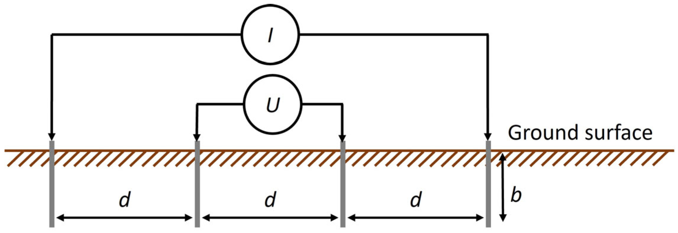
Figure 1. Placement of electrodes for the Wenner method.
Applsci 15 01420 g001
Figure 2. (a) N- and (b) three-layered soil model.
Applsci 15 01420 g002
Figure 3. (a) Approach of using two directions of measurement and (b) approach by dividing the area into smaller parts.
Applsci 15 01420 g003
Figure 4. (a) First step—division of the area; (b) second step—Wenner’s method measurements; (c) third step—measurements used for subareas; and (d) fourth step—soil parameters for the subareas of the FEM model.
Applsci 15 01420 g004
Figure 5. Three-dimensional FEM model used for the tests.
Applsci 15 01420 g005
Figure 6. Two-dimensional cross-section of the FEM test model at the ground surface with marked dimensions.
Applsci 15 01420 g006
Figure 7. Algorithm of the soil parameters’ calculation procedure.
Applsci 15 01420 g007
Figure 8. Mean OF values for all five optimization methods and all nine subareas.
Applsci 15 01420 g008
Figure 9. Convergence of the evolutionary methods for (a) AD subarea, (b) AE subarea, (c) AF subarea, (d) BD subarea, (e) BE subarea, (f) BF subarea, (g) CD subarea, (h) CE subarea and (i) CF subarea.
Applsci 15 01420 g009
Figure 10. Algorithm presenting Short-Term Memory Assistance (STMA).
Applsci 15 01420 g010
Figure 11. Algorithm presenting Long-Term Memory Assistance (LTMA).
Applsci 15 01420 g011
Figure 12. Mean OFs for different soil models in different subareas.
Applsci 15 01420 g012
Figure 13. (a) Basic and (b) determined FEM model.
Applsci 15 01420 g013
Figure 14. Apparent resistivity at lines (a) Meas. A, (b) Meas. B, (c) Meas. C, (d) Meas. D, (e) Meas. E and (f) Meas. F.
Applsci 15 01420 g014
Figure 15. (a) Geological anomaly and (b) determined FEM model using three-layered soil for each subarea.
Applsci 15 01420 g015
Table 1. Parameters’ limits for the three-layered soil model.
ParameterLower LimitUpper Limit
Resistance of the first soil layer ρ1 (Ωm)33500
Thickness of the first soil layer h1 (m)0.160
Resistance of the second soil layer ρ2 (Ωm)33500
Thickness of the first soil layer h2 (m)0.160
Resistance of the third soil layer ρ3 (Ωm)33500
Table 2. Calculation parameters using different methods.
MethodSoil ModelNumber of Parameters (P)Population Number (NP)Number of IterationsObjective Function Evaluations
DE/rand/1/exp, DE/rand/2/exp, DE/best/1/binThree-layeredP
5
NP = 6 × P
30
ITER
600
OFEs = NP × ITER
18,000
TLBOThree-layeredP
5
NP = 6 × P
30
ITER
300
OFEs = NP × 2 × ITER
18,000
ABCThree-layered5NP = 6 × P
30
ITER
≤600
OFEs = NP × ITER + scouts
Max. 18,000
Table 3. Calculated apparent resistivity for lines A, B, C, D, E, and F are shown in Figure 4b.
d (m)Line A
ρ (Ωm)
Line B
ρ (Ωm)
Line C
ρ (Ωm)
Line D
ρ (Ωm)
Line E
ρ (Ωm)
Line F
ρ (Ωm)
1183.22183.55184.13183.72184.22183.97
2210.06209.85215.69210.29211.15210.85
3208.67208.75232.01209.06209.62209.27
4205.59205.72258.97206.05205.88205.68
5203.32203.09257.80203.86204.15203.55
10199.53200.65227.38210.76202.30199.95
15199.32201.59366.08249.97207.96199.82
20199.25203.11342.29220.49211.24199.71
25198.70204.64292.28196.82209.60199.34
30198.13205.35255.03180.20207.68198.37
35197.13205.68231.60168.14205.57197.39
40195.79204.92216.43158.44203.47196.03
45191.95203.68206.72165.72202.14194.33
50194.04201.78199.47174.25200.22192.11
55189.15199.29193.47176.86198.49189.30
60186.08196.08187.89176.48195.08186.32
65182.25192.31182.19173.90191.16182.49
70177.93187.65175.79169.26186.10178.19
75172.78182.120167.63160.95179.60173.16
80166.92175.71155.97146.07171.77167.25
Table 4. Average apparent resistivity for the nine subareas presented in Figure 4c.
d (m)Area AD
ρ (Ωm)
Area AE
ρ (Ωm)
Area AF
ρ (Ωm)
Area BD
ρ (Ωm)
Area BE
ρ (Ωm)
Area BF
ρ (Ωm)
Area CD
ρ (Ωm)
Area CE
ρ (Ωm)
Area CF
ρ (Ωm)
1183.47183.72183.60183.64183.88183.76183.93184.17184.05
2210.17210.61210.45210.07210.50210.35212.99213.32213.27
3208.86209.14208.97208.90209.18209.01220.53220.81220.64
4205.82205.74205.64205.88205.80205.70232.51232.43232.33
5203.59203.73203.44203.48203.62203.32230.83230.97230.68
10205.14200.91199.74205.70201.47200.30219.07214.84213.67
15224.65203.63199.57225.78204.78200.70308.02287.02282.95
20209.87205.24199.48211.80207.17201.41281.39276.77271.00
25197.76204.15199.02200.73207.12201.99244.55250.94245.81
30189.16202.91198.25192.77206.52201.86217.61231.36226.70
35182.63201.34197.26186.91205.62201.53199.87218.58214.49
40177.12199.63195.91181.68204.19200.48187.44209.995206.23
45179.88198.09194.19184.70202.91199.01186.22204.43200.52
50183.10196.09192.03188.01201.00196.94186.86199.85195.79
55183.00193.77189.22188.07198.84194.29185.16195.92191.38
60181.28190.58186.20186.28195.58191.20182.19191.49187.11
65178.07186.70182.37183.11191.74187.40178.04186.67182.34
70173.59182.01178.06178.45186.87182.92172.52180.95176.99
75166.87176.19172.97171.57180.90177.68164.29173.62170.40
80156.50169.35167.08160.89173.74171.48151.02163.87161.61
Table 5. OF and best value of the calculated parameters for 50 independent runs for the AD subarea.
OF and Method
Parameters DE/rand/1/expDE/rand/2/expDE/best/1/binTLBOABC
B3.08963.08963.08962.85822.8489
OF (%)W3.75103.45423.86533.50353.3519
M3.24003.18723.38343.17853.0170
SD2.0186 × 10−11.0763 × 10−12.5406 × 10−11.4714 × 10−11.4260 × 10−1
ρ1 (Ωm)B206.54206.54206.5459.0157.51
h1 (m)B16.8516.8616.850.100.10
ρ2 (Ωm)B184.92184.92184.92208.40209.08
h2 (m)B99.8299.8299.8221.6817.14
ρ3 (Ωm)B5.005.005.00163.14167.26
Table 6. OF and best value of the calculated parameters for 50 independent runs for the AE subarea.
OF and Method
Parameters DE/rand/1/expDE/rand/2/expDE/best/1/binTLBOABC
B1.21651.21671.02961.03041.0326
OF (%)W1.37791.35931.36601.35351.3074
M1.28981.23841.31621.30241.1256
SD6.0563 × 10−24.7049 × 10−27.4706 × 10−26.1949 × 10−28.1256 × 10−2
ρ1 (Ωm)B203.73203.7361.8261.8184.33
h1 (m)B55.9354.540.100.100.14
ρ2 (Ωm)B3457.34655.78205.77205.77205.82
h2 (m)B2.5013.60100.00100.00100.00
Table 7. OF and best value of the calculated parameters for 50 independent runs for the AF subarea.
OF and Method
Parameters DE/rand/1/expDE/rand/2/expDE/best/1/binTLBOABC
B1.25601.19471.19471.25601.1974
OF (%)W1.44501.44081.43321.42111.3651
M1.37881.29721.38261.37691.2462
SD6.6917 × 10−27.2750 × 10−26.7640 × 10−25.6695 × 10−24.0584 × 10−2
ρ1 (Ωm)B199.7767.6267.62199.7767.76
h1 (m)B60.170.100.1060.170.10
ρ2 (Ωm)B2940.90201.76201.763494.85201.86
h2 (m)B2.76100.00100.002.32100.00
ρ3 (Ωm)B5.0023.2123.215.0022.84
Table 8. OF and best value of the calculated parameters for 50 independent runs for the BD subarea.
OF and Method
Parameters DE/rand/1/expDE/rand/2/expDE/best/1/binTLBOABC
B3.04022.80712.80713.04022.8106
OF (%)W3.34733.34723.34743.34743.1828
M3.20353.21483.26983.26732.9380
SD1.4430 × 10−11.5686 × 10−11.3305 × 10−11.1933 × 10−19.7723 × 10−2
ρ1 (Ωm)B206.6258.3358.33206.6158.55
h1 (m)B17.030.100.1017.090.10
ρ2 (Ωm)B192.41208.53208.53192.37208.57
h2 (m)B97.2718.6918.6997.2419.24
ρ3 (Ωm)B5.00171.81171.815.00171.38
Table 9. OF and best value of the calculated parameters for 50 independent runs for the BE subarea.
OF and Method
Parameters DE/rand/1/expDE/rand/2/expDE/best/1/binTLBOABC
B1.19661.19691.19661.19671.1973
OF (%)W1.72801.67381.74091.67441.4790
M1.25701.21661.51571.39121.2340
SD1.6158 × 10−19.3316 × 10−22.3814 × 10−12.2395 × 10−14.5144 × 10−2
ρ1 (Ωm)B204.30204.42204.30204.30204.42
h1 (m)B48.6248.2648.6248.6348.81
ρ2 (Ωm)B3347.501124.283495.953499.373353.95
h2 (m)B3.019.032.882.883.00
ρ3 (Ωm)B5.005.005.005.005.00
Table 10. OF and best value of the calculated parameters for 50 independent runs for the BF subarea.
OF and Method
Parameters DE/rand/1/expDE/rand/2/expDE/best/1/binTLBOABC
B1.15441.15441.15441.15441.1658
OF (%)W1.61531.58503.87521.56991.4157
M1.19971.17971.50441.42561.2230
SD1.3042 × 10−19.7386 × 10−23.8659 × 10−11.7582 × 10−15.1185 × 10−2
ρ1 (Ωm)B201.39201.44201.38201.39201.70
h1 (m)B52.2952.3352.2952.3052.52
ρ2 (Ωm)B3473.142659.333500.003499.541011.04
h2 (m)B2.743.572.712.719.30
ρ3 (Ωm)B5.005.005.005.006.64
Table 11. OF and best value of the calculated parameters for 50 independent runs for the CD subarea.
OF and Method
Parameters DE/rand/1/expDE/rand/2/expDE/best/1/binTLBOABC
B6.42486.42484.92106.42504.9306
OF (%)W6.76756.54478.49546.69566.1153
M6.51366.50946.60396.52185.2753
SD5.4329 × 10−24.6391 × 10−24.6255 × 10−13.9922 × 10−22.9209 × 10−1
ρ1 (Ωm)B220.56220.5640.99220.5678.72
h1 (m)B24.2224.220.1024.310.20
ρ2 (Ωm)B187.95187.96235.73187.76235.96
h2 (m)B76.6076.6035.6317.6230.35
ρ3 (Ωm)B5.005.00122.645.02134.77
Table 12. OF and best value of the calculated parameters for 50 independent runs for the CE subarea.
OF and Method
Parameters DE/rand/1/expDE/rand/2/expDE/best/1/binTLBOABC
B5.36823.96053.51594.57173.5846
OF (%)W5.37355.37356.42055.37005.3712
M5.36925.34105.31065.35324.0532
SD6.5976 × 10−41.9721 × 10−14.6429 × 10−11.1165 × 10−14.1656 × 10−1
ρ1 (Ωm)B220.8242.52135.81213.6141.59
h1 (m)B83.570.100.455.580.10
ρ2 (Ωm)B31.52232.40238.61266.98235.19
h2 (m)B47.3280.0043.7322.5446.70
ρ3 (Ωm)B5.005.00113.84146.29109.72
Table 13. OF and best value of the calculated parameters for 50 independent runs for the CF subarea.
OF and Method
Parameters DE/rand/1/expDE/rand/2/expDE/best/1/binTLBOABC
B5.13055.13063.30734.14093.3198
OF (%)W5.21625.14406.69675.21625.1539
M5.14345.14155.09125.11833.7941
SD1.0909 × 10−23.91066 × 10−34.2136 × 10−11.5246 × 10−14.0815 × 10−1
ρ1 (Ωm)B220.65220.66120.0445.60122.10
h1 (m)B46.3746.610.360.100.37
ρ2 (Ωm)B160.29159.27236.32229.55236.72
h2 (m)B64.9965.2340.0379.5838.78
ρ3 (Ωm)B5.005.00120.035.46123.51
Table 14. Mean calculation times for 50 independent runs.
Calculation Method
Times/SubareaDE/rand/1/expDE/rand/2/expDE/best/1/binTLBOABC
t (s)/AD4.224.8816.677.2533.25
t (s)/AE4.835.3417.905.4539.12
t (s)/AF14.6014.9514.274.0141.07
t (s)/BD5.1115.2030.875.7935.66
t (s)/BE5.185.9611.229.2033.40
t (s)/BF4.505.0529.053.7336.35
t (s)/CD4.315.8615.923.8032.99
t (s)/CE5.0013.8426.815.1931.43
t (s)/CF4.705.3235.776.0034.34
Table 15. Precisions of the parameters that determine the identification of duplications.
ParameterMaximum Difference
ρ1, ρ2, ρ30.1 mΩm
h1, h20.1 mm
Table 16. Mean calculation times, deviations of calculation times, and duplications for 50 independent runs.
SubareaABC
t(s)
ABC + STMA
t(s)
Deviation of t
Using STMA (%)
Duplications STMAABC + LTMA
t(s)
Deviation of t
Using LTMA (%)
Duplications LTMA
AD33.2528.0184.2155730.3991.42655
AE39.1227.3369.9170725.9266.32551
AF41.0728.7770.1164129.8072.62615
BD35.6631.1887.4167030.6886.02738
BE33.4026.8480.4167725.9377.62484
BF36.3528.7479.1154926.8273.82454
CD32.9927.5583.5193029.3188.82852
CE31.4328.3390.1173627.3687.12650
CF34.3423.1367.4167523.3367.92784
Mean35.2927.7679.1%168227.7379.0%2643
Table 17. Test of three-, four-, five-, and six-layered models using 50 independent runs for each model and for each area.
Subarea Soil Model
Three LayersFour LayersFive LayersSix Layers
B2.84892.80212.66062.3731
ADW3.35193.25763.25973.4385
M3.01703.03243.02983.0313
SD1.4260 × 10−11.0472 × 10−11.1070 × 10−11.8770 × 10⁻¹
B1.03261.02290.94350.7258
AEW1.30741.34411.31861.4264
M1.12561.19191.15021.2290
SD8.1256 × 10−27.3115 × 10−21.0621 × 10−11.2140 × 10⁻¹
B1.19741.03780.80370.8057
AFW1.36511.37031.46331.5694
M1.24621.19841.20581.2461
SD4.0584 × 10−28.2700 × 10−21.1100 × 10−11.6308 × 10⁻¹
B2.81062.72372.53552.4723
BDW3.18283.26633.21403.2300
M2.93802.96972.91992.8683
SD9.7723 × 10−29.6893 × 10−21.6189 × 10−11.8302 × 10⁻¹
B1.19730.92740.88950.8382
BEW1.47901.24441.28601.3274
M1.23401.15091.07341.1341
SD4.5144 × 10−29.8441 × 10−21.2563 × 10−11.2988 × 10⁻¹
B1.16580.98080.638340.8348
BFW1.41571.29431.25211.4245
M1.22301.13591.09091.1736
SD5.1185 × 10−25.9807 × 10−21.0602 × 10−11.1372 × 10⁻¹
B4.93064.59024.83764.9021
CDW6.11536.41916.57686.5309
M5.27535.40915.46525.4593
SD2.9209 × 10−14.2134 × 10−14.5797 × 10−14.4843 × 10⁻¹
B3.58463.27223.23293.4347
CEW5.37125.24034.96035.4556
M4.05323.91153.91754.0276
SD4.1656 × 10−13.8760 × 10−13.1435 × 10−14.0025 × 10⁻¹
B3.31982.99873.39012.7103
CFW5.15395.10605.03555.2276
M3.79413.81533.77523.9706
SD4.0815 × 10−14.5375 × 10−13.9664 × 10−15.4033 × 10⁻¹
Disclaimer/Publisher’s Note: The statements, opinions and data contained in all publications are solely those of the individual author(s) and contributor(s) and not of MDPI and/or the editor(s). MDPI and/or the editor(s) disclaim responsibility for any injury to people or property resulting from any ideas, methods, instructions or products referred to in the content.