Low-Energy Path Planning Method of Electrically Driven Heavy-Duty Six-Legged Robot Based on Improved A* Algorithm

Abstract

Compared to the traditional non-load-bearing multi-legged robots, the heavy-duty multi-legged robots typically not only have larger body weight, larger volume, and larger load ratio but also require greater energy dissipation. Traditional path planning often focuses on the problem of finding the shortest path. However, the substantial load capacity and multi-jointed structure of heavy-duty multi-legged robots impose stringent requirements on path smoothness. Consequently, the smoothness requirement makes the traditional A* algorithm unsuitable for applications where low-energy operation is critical. An improved low-energy path planning method based on the A* algorithm is presented for an electrically driven heavy-duty six-legged robot. Then, the environment is discretized by using the grid method to facilitate path searching. To address the path zigzagging problem caused by the traditional A* algorithm, the Bézier curve smoothing technique is adopted. The continuous curvature transitions are employed to significantly improve the smoothness of path. The heuristic function in the A* algorithm is enhanced through a dynamic weight adjustment mechanism. The nonlinear suppression strategy is introduced to prevent data changes and improve the robustness of the algorithm. The effectiveness of the proposed method is verified through the MATLAB simulation platform system. The simulation experiments show that, in various environments with different obstacle densities (0.17–0.37%), compared with the traditional A* algorithm, the method proposed in this paper reduces the average path length by 7.2%, the number of turning points by 25.9%, and the energy consumption by 5.75%. The proposed improved A* algorithm can significantly overcome the problem of insufficient smoothness in traditional A* algorithms and reduce the number of nodes generated by the control data stack, which improves the optimization efficiency during path planning. As a result, the heavy-duty six-legged robots can walk farther and operate for longer periods of time while carrying the limited energy sources.

1. Introduction

Mobile robots, due to their advantages of intelligence and strong execution capabilities, have garnered widespread attention and application in high-profile industries such as aerospace manufacturing and intelligent manufacturing [1,2,3]. However, traditional autonomous mobile robots have limited carrying capacity. Thus, they cannot stably perform control tasks under high-duty conditions. Furthermore, under the constraint of limited control costs, unconstrained data transmission can inevitably lead to redundancy and interruptions. As tasks become more complex and demanding, especially in unstructured environments, the limitations of traditional mobile robots in terms of load capacity and energy endurance are revealed.

The six-legged robots, with their biomimetic structure and multi degree of freedom advantages, have shown great potential for applications in unstructured environments such as disaster relief and planetary exploration. Due to the superior characteristics such as higher stability, higher load capacity, higher mobility, and more extensive application scenarios, the electrically driven heavy-duty six-legged robots have gradually attracted the research interest of scholars. For example, Gao et al. [4] made fundamental contributions in the mechanism synthesis and gait planning of the type of robot; Ding et al. [5] conducted in-depth research on bionic learning and motion control; Zhuang et al. [6] systematically analyzed its power consumption characteristics, joint speed range, and conducted gait planning research; Gao et al. [7] conducted in-depth research on the configuration synthesis of walking legs; etc. The working environments of electrically driven heavy-duty six-legged robots require robots to autonomously navigate in extremely rugged and complex terrains. However, the autonomous movement of electrically driven heavy-duty six-legged robots is an extremely complex problem. It is not a simple geometric path search, but a motion planning problem that deeply integrates gait generation, foothold selection, and stability control. The increase in robot degrees of freedom leads to a combinatorial explosion in the planning space, which is the curse of dimensionality and excludes the use of exhaustive search algorithms. Moreover, the geometrically shortest path is often not executable due to the lack of stable landing points. Then, a serious challenge is created, which is how to maximize the working hours under strict onboard energy constraints.

The global path planning is an advanced decision-making module whose core task is to identify safe areas that can be passed through at a macro level, such as relatively flat and sturdy terrain, and plan a globally feasible path for the robot to reach the target point, thereby providing a leading trajectory for the ankle point sequence planning at the bottom layer [8]. Although the existing hierarchical planning methods have universality, they are insufficient for the heavy-duty six-legged robots. The heavy load characteristics require higher stability and many legs, so the energy consumption of robots during movement is much higher than that of normal bipedal robots. When encountering turning situations, the body of the heavy-duty six-legged robot needs to constantly adjust its posture. Such frequent posture adjustments significantly increase the energy consumption of the robot when making turns. Additionally, the six legs require numerous movements to maintain balance and adapt to the terrain. In order to ensure that the generated global path not only avoids obstacles but also significantly improves the overall planning efficiency and cost utilization, it is necessary to propose a low-energy hierarchical path planning framework and introduce a cost evaluation model during the global planning stage.

Currently, there are some existing global path planning algorithms, such as the Dijkstra algorithm, RRT algorithm, D* algorithm and A* algorithm. Then, Alshammrei et al. [9] proposed an optimal collision avoidance algorithm based on an improved Dijkstra algorithm. Zhou and Huang [10] established a Dijkstra algorithm based automatic guidance path planning model to achieve the application of automatic guidance in airport baggage loading scenarios. Sundarraj et al. [11] used a weighted particle swarm optimization Dijkstra algorithm to determine the most efficient and secure path between the source and target. Noreen et al. [12] compared the advantages and disadvantages of RRT algorithms in various environments to simulate the implementation of path planning. Zhang et al. [13] proposed an improved RRT algorithm to refine the boundary nodes in the joint space to prevent excessive search of the configuration node space. Maurovi’c et al. [14] used a D* shortest path graph search algorithm to improve the exploration of highly dynamic environments with moving obstacles. Yang and Teng [15] designed an A* algorithm that enhanced dynamic windows to track deviation angles and quickly captured target motion points. Xiang et al. [16] established an improved A* algorithm combined with greedy algorithm as a multi-objective path planning strategy to remove unnecessary nodes in the A* algorithm. Liu et al. [17] presented an improved A* algorithm for searching priority and rule path nodes to handle complex obstacles. Zhuang et al. [18] optimized and reconstructed the grid map according to the real-time game rules of Go and proposed a multi-destination global path planning algorithm based on the optimal obstacle value. To navigate through complex wilderness environments, Xu P. et al. [19] applied a sliding search algorithm to six-legged robots for path planning.

However, there are significant differences in energy consumption characteristics between the multi-legged robots and the traditional wheel robots. Frequent turning, lateral movements, and other behaviors require coordination of more joint movements. The energy consumption of the six-legged robots is much higher than that of straight walking. When driving on terrains with different slopes and ground friction coefficients, the torque and power required by the drive motor vary significantly. The six-legged robots require more energy to climb slopes than to walk on flat ground. The gait switching to adapt to the different speeds or terrains can also result in additional energy consumption. However, the optimality of the classic A* algorithm is solely based on the criterion of shortest path length. For the six-legged robots with limited endurance and complex motion modes, that is not the only or optimal definition of the optimal solution. Therefore, a path with the shortest geometric length may involve multiple sharp turns, steep climbs, or complex terrain. The total energy consumption may be much higher than a slightly longer but flat and straight path. The six-legged robots rely on onboard batteries and have a limited duration for their tasks. Therefore, reducing energy consumption and shortening the path length are equally important. Therefore, it is necessary to design an A* algorithm that can combine low-energy control. At present, research on low-energy control has also been conducted in the field of path planning. Liu and Sun [20] established an energy consumption model for calculating kinetic energy conversion and overcoming traction resistance to generate energy-saving paths. Yao et al. [21] established an energy consumption model based on a driving motor for the evaluation function of the extended dynamic window method. Wang et al. [22] proposed a real-time low-energy path planning generation method based on parallel deep learning to reduce the energy consumption of a given production line task. Soijoyo and Wardoyo [23] studied an improved heuristic A* algorithm based on energy optimization, aiming to identify path trajectories under energy-saving conditions.

At present, the research on the six-legged robots can still be improved in terms of path planning and energy consumption. Traditional algorithms have problems such as low search efficiency and insufficient path smoothness. Therefore, in recent years, researchers have proposed various improvement schemes. Wang et al. [24] improved the path planning and tracking framework for the six-legged robots based on the A* algorithm and model predictive control. They introduced an artificial potential field (APF) factor into the evaluation function to generate a safe and collision-free initial path. Chen et al. [25] proposed a Particle Swarm Optimization (PSO)-guided Double Deep Q-Network (DDQN) approach. The proposed algorithm incorporates the PSO algorithm to supplant the traditional random selection strategy. Due to the complex structure and high control difficulty of six-legged robots, the issue of energy consumption has become a key bottleneck restricting their long-term operation. Wang et al. [26] established a quadratic-programming force-distribution controller. The controller reduced the energy consumption by optimizing the instantaneous power of the robot at each time step. Yang et al. [27] proposed an adaptive fuzzy impedance algorithm for the real-time force-position composite control of foot position adjustment to reduce the steady-state force tracking error caused by terrain stiffness, thereby ensuring stability of body by tracking variable foot-end forces. Hu et al. [28] sought to investigate the effect of actuation patterns on the power consumption of legged robots that perform motion in a quasi-static manner. The power consumption model of legged robots considering actuation patterns was deduced. At present, there have been some studies on path planning and energy consumption of six-legged robots. However, in the field of path planning algorithms, the mechanical characteristics of the six-legged robots have not been well integrated with the algorithms. The traditional A* algorithm excels at finding the geometrically shortest paths. Some of the current energy consumption calculation models lack the inclusion of dynamic factors such as turning losses and terrain-related costs. The gap between the path geometry planning and the actual energy consumption is precisely what the work aims to bridge. Based on the problems mentioned above and the previous basic research on the heavy-duty muti-legged robot. An electrically driven heavy-duty six-legged robot is considered as an example in the paper to present an analysis method of the low-energy path planning based on improved A* Algorithm, which is to study the characteristics of higher energy consumption during robot turning compared to straight walking, and to evaluate the energy consumption required for robot path planning using the improved A* algorithm.

Traditional path smoothing methods often only focus on geometric characteristics and do not consider energy consumption as the optimization objective. The existing algorithms that have improved upon the A* algorithm lack consideration of the special energy consumption characteristics of six-legged robots, such as the significantly higher energy consumption for turning compared to linear motion. No quantitative relationship model between energy consumption and path geometric characteristics has been established. The influence of the dynamic constraints of the robot in heavy-load conditions on energy consumption has also been ignored.

Based on the above problems and analysis, an electrically driven heavy-duty six-legged robot is taken as the research object, aiming to propose a low-energy consumption path planning method. The paper aims to achieve three core objectives. Firstly, a robot energy consumption model is established that fully considers both straight-line walking and turning movements. Secondly, the traditional A* algorithm is improved through the integration of a path smoothing mechanism. Finally, the effectiveness of the proposed method is verified through simulation experiments, demonstrating its ability to reduce path length, decrease the number of turns, and save energy.

The paper can be organized as follows. In Section 2, the path of robot is divided into the straight walking segments and turning segments to systematically establish the energy consumption model of robot. In Section 3, three key improvements are made to the traditional A* algorithm, namely dynamic weight adjustment, Bézier curve smoothing of the path, and an improved heuristic function. In Section 4, the simulation experiments are conducted under different obstacle rate scenarios, which are employed to compare the performance of the improved A*algorithm with the traditional A* algorithm in terms of path length, number of turning points, and energy consumption. Meanwhile, the effectiveness and superiority of the proposed method are verified. Finally, the main conclusions are offered in Section 5.

2. Establishment of Energy Consumption Model for Electrically Driven Heavy-Duty Six-Legged Robot

To enable energy-efficient path planning, an accurate and computationally tractable energy consumption model is established in this section, which will provide a theoretical basis for the cost function design in the next section’s algorithm improvement. The unique characteristics of the electrically driven heavy-duty six-legged robot are demonstrated. The servo motors are employed for the prototype of robot, which can provide the high load capacity and superior obstacle-crossing performance. The six-legged configuration offers inherent static stability and enhances adaptability to complex terrains. All critical joints are equipped with high-precision sensors. Therefore, the system is suitable for heavy-duty operations and autonomous walking experiments in challenging environments. The prototype of electrically driven heavy-duty six-legged robot is shown in Figure 1.

Figure 1. Prototype of electrically driven heavy-duty six-legged robot [6].

The electrically driven heavy-duty six-legged robot features a total body mass of 310 kg, with compact external dimensions measuring 1.4 m in length, 1.4 m in width, and 1.5 m in height in its standard operational posture. Designed for substantial load-bearing applications, the system supports a payload capacity of 155 kg and demonstrates robust mobility over challenging terrain. The key mobility specifications include the ability to surmount obstacles up to 0.3 m in height, traverse ditches with widths up to 0.3 m, achieve a maximum walking speed of 0.6 km/h, and navigate slopes with inclines up to 35 degrees. The leg actuation system incorporates specialized joint motors optimized for powerful and coordinated movement. The ankle joint is driven by a 250 W motor, the hip joint by a 400 W motor, and the knee joint by a 250 W motor, ensuring efficient force distribution and stable locomotion under heavy loads. The configuration enables the heavy-duty six-legged robot to maintain balance and traction across uneven surfaces while carrying significant payloads.

For the convenience of elaborating the content in this paper, the electrically driven heavy-duty six-legged robot is referred to as the heavy-duty six-legged robot. A mathematical model for the path energy consumption of heavy-duty six-legged robots is proposed. It aims to quantitatively evaluate the energy efficiency performance of different path planning algorithms under the load conditions. The core objective of the model is to quantitatively analyze and compare the expected energy consumption of paths planned by different algorithms in a grid map. Specifically, the total energy consumption E_all is defined as the sum of energy consumption of all straight-line segments E_line and corner segments E_turn in the path. Then

$$E_{\mathrm{all}}=E_{\mathrm{line}}+E_{\mathrm{turn}}$$

(1)

In order to make the theoretical analysis more rigorous, the following assumptions are proposed for a more detailed analysis.

Remark 1.

The torso of the electrically driven heavy-duty six-legged robot is a rigid structure. The robot adopts a symmetrical gait for straight walking or turning walking.

2.1. Establishment of Energy Consumption Model for Straight Walking

The energy consumption model aims to predict the expected energy consumption of robots by integrating its internal actuation dynamics and external environmental conditions. Meanwhile, the energy expended during straight-line walking is primarily attributed to the motor’s electrical energy demand, which is used to drive the robot’s motion and overcome resistive forces to maintain a constant velocity. The components of energy expenditure establish the baseline for the overall power model, as they capture the fundamental mechanical and electrical losses during unconstrained locomotion. By accurately quantifying baseline of energy consumption, the model of energy consumption provides a critical foundation for evaluating and optimizing the overall energy efficiency of the robotic system across various operational scenarios.

Assume that the travel distance of the robot in the grid map is L, measured in grid units, with its total mass including payload denoted as $m_{\mathrm{load}}$, moving speed as v, and ground friction coefficient as μ. Against this context, it is first essential to clarify the definitions of each physical quantity in the energy consumption formula: g represents gravitational acceleration, with a value of 9.8 m/s²; C_d is the drag coefficient associated with the robot’s body shape; A denotes the frontal area, with a unit of m²; ρ stands for air density, with a unit of kg/m³; and K_m is the motor power coefficient obtained by fitting the motor characteristic curve, with a unit of W/(m/s). Based on these definitions, the energy consumption of the robot in this scenario can be quantitatively expressed as follows. Then

$$E_{\mathrm{line}}=\mu m_{\mathrm{load}}gL+{\displaystyle \frac{1}{2}}{C}_{d}A\rho {\nu }^{2}L+K_{\mathrm{m}}vL$$

(2)

Many existing energy consumption models assume that robots move in straight lines across ideal flat and frictionless surfaces. However, the ground conditions in reality are complex and diverse, often involving slopes, uneven terrain, and different friction coefficients. To enhance the rigor of theoretical analysis, the following assumptions are introduced to support a more detailed investigation. When walking on different materials such as outdoor grass, sand, or indoor carpets, the heavy-duty six-legged robot needs to overcome different resistances. These factors are often neglected in idealized assumptions, leading to deviations between the model and the actual energy consumption.

Remark 2.

The terrain slope effect is approximated as zero in this study due to the two-dimensional grid-based framework employed for path planning. Although the slope theoretically affects energy consumption, the grid method itself focuses on plane path attributes such as node connectivity and local smoothness and is unable to directly capture altitude changes or the differences in three-dimensional terrain. To align with the primary research objective of optimizing path smoothness rather than addressing complex 3D terrain effects, slope is explicitly set to zero in the energy consumption model throughout simulations. The simplification is methodologically justified by the framework’s limitation in representing vertical terrain features, ensuring the study remains focused on its core goal of path optimization under planar constraints.

All parameters in Section 2.1 are set based on the physical characteristics of the actual robot platform. The key parameters are acquired through experimental measurements or device manuals, ensuring the fundamental reliability of the model.

2.2. Establishment of Energy Consumption Model for Turning Walking

The distinction is of crucial importance in understanding the energy dynamics of legged robotic systems. The multi-legged robots are different from wheeled vehicles in that they must perform a series of complex coordinated movements to achieve the directional change. The maneuvers often involve sequential leg lifting, repositioning, and body reorientation. The movements collectively introduce significant inertial losses and internal friction within articulated actuators. Such energy dissipation arises from accelerating and decelerating the robot’s mass and appendages. Moreover, such changes are poorly captured by purely distance-based metrics, underscoring the need for motion-aware energy modeling.

However, the actual application scenarios include disaster response, logistical support, planetary exploration, and other unstructured environments. In addition to traversing straight paths, the electrically driven heavy-duty six-legged robot is often required to execute turning maneuvers. The main body of robot and weight of load are quite heavy. The kinematics of the multi-joint leg mechanism is complex. The energy expenditure associated with turning is markedly higher than that of the straight-line motion. The turning strategies of the electrically driven heavy-duty six-legged robot fundamentally differ from the wheeled platforms. The electrically driven heavy-duty six-legged robot demands continuous adjustment of the foot position, careful stability management, and compensatory body motions to achieve curvature while maintaining the body balance. The top-view schematic, which illustrates the pose and leg trajectory of the electrically driven heavy-duty six-legged robot during a typical turning operation, is provided in Figure 2.

Figure 2. Top-view schematic of electrically driven heavy-duty six-legged robot during turning.

The turning action requires overcoming the inertia barrier and the sliding friction between the ground and the foot ends. The energy consumption of the electrically driven heavy-duty six-legged robot is nonlinearly related to the turning angle $\Delta \theta$. Then

$$\left\{\begin{array}{l}{E}_{\mathrm{turn}}\hspace{0.5em}\approx n\left({\displaystyle \frac{1}{2}}{I}_{\mathrm{eff}}\hspace{0.5em}{\left(\Delta \dot{\theta }\right)}^2+{\mu }_{\mathrm{s}}{m}_{\mathrm{load}}gR\Delta \theta \right)\\ I_{\mathrm{eff}}=I_{\mathrm{body}}+m_{\mathrm{load}}{d}_{\mathrm{load}}^2\\ \Delta \dot{\theta }={\displaystyle \frac{\Delta \theta }{\Delta t}}\end{array}\right.$$

(3)

where I_eff is the equivalent moment of inertia; I_body is the rotational inertia of the robot’s body; d_load represents the offset of the loads center of mass; $\Delta \dot{\theta }$ is the average angular velocity, rad/s²; ${\mu }_{\mathrm{s}}$ is the steering sliding friction coefficient, ${\mu }_{\mathrm{s}}>\mu$; and R is the turning radius, m, which is related to gait.

Unlike distance-based simple models, the proposed turning energy model more accurately reflects actual motion characteristics through parameters like equivalent moment of inertia I_eff and sliding friction coefficient μ_s.

Compared with the simplistic distance-based models, the proposed energy consumption model can achieve more accurate estimation of the energy consumption, which is crucial for evaluating and comparing the performance of different path planning algorithms. In summary, the energy consumption model is applied to a set of computational examples by using data from the electrically driven heavy-duty six-legged robot. The key parameters of electrically driven heavy-duty six-legged robot for the simulations are provided in Table 1.

Table 1. Parameters of electrically driven heavy-duty six-legged robot.

Parameters	Symbol	Value
Total weight	$m_{\mathrm{load}}$	310 kg
Load center offset quantity	$d_{\mathrm{load}}$	0
Body moment of inertia	$I_{\mathrm{body}}$	90 kg·m2
Gravitational acceleration	$g$	9.8 m/s2
Air density	$\rho$	1.2 kg/m3
Linear walking speed	$v$	1 m/s
Radius of turning circle	$R$	1.5 m
Ground friction coefficient	$\mu$	0.4
Sliding friction coefficient for steering	${\mu }_s$	0.5
Motor power factor	$K_m$	1.6 W/(m/s)
Windward area	$A$	1.3 m
Drag coefficient	$C_d$	1

Note: The friction coefficient μ can be obtained based on experimental measurements of ground materials; the mass m represents the total mass of the entire robot and its load; the motor parameter K_m can be determined by fitting the motor characteristic curve.

3. Low-Energy Optimal Path Planning Method Based on Improved A* Algorithm

Based on the energy consumption model established in Section 2, three key improvements are made to the traditional A* algorithm. The efficiency of the A* algorithm is largely attributed to its strategic use of a priority queue. The mechanism systematically selects the most promising nodes for expansion based on a cost minimization strategy. During each iteration, the algorithm evaluates adjacent nodes from the current position, computes their corresponding cost functions, and inserts them into the priority queue according to their priority values. The iterative process continues until the target node is successfully reached or the entire search space has been exhaustively explored.

In continuation from the previous discussion on the overall framework of the improved A* algorithm, the paragraph delves into the specific methodological details. To facilitate understanding, key terms are defined herein: a motion graph refers to a graph structure where nodes represent feasible robot poses, and edges represent viable motion trajectories between poses, enabling efficient path search in complex environments. The open set denotes the collection of nodes awaiting exploration in the A* algorithm, dynamically guiding the search process toward promising paths while ensuring completeness. These elements are fundamental to the algorithm’s operation, bridging the high-level strategy with low-level implementation. The environment is abstracted as a motion graph where nodes represent feasible positions and edges represent movement costs. The algorithm maintains an Open Set and a Closed Set to systematically search for the optimal path. Each node in the motion graph begins in an undiscovered state. The node is moved into the open set on its first visit, indicating that it has been discovered but not yet expanded. Once all its neighbors have been evaluated, the node is moved to the closed set and marked as fully expanded. Although the state transition mechanism is conceptually simple, the search strategy remains highly effective. The heuristic functions are acceptable under normal circumstances, which means they never overestimate the true cost of the goal. As a result, the A* algorithm is guaranteed to produce an optimal solution.

Section 3 details three core modifications to the conventional A* algorithm, aimed at incorporating an energy consumption model and substantially enhancing path smoothness. These adaptations maintain the optimality and completeness of the original algorithm, while customizing energy-aware navigation for the heavy-duty six-legged robot. The key integrated factors include motor efficiency, ground friction, terrain impact, and motion-induced costs such as acceleration and turning. Additionally, the improved A* algorithm integrates mechanisms such as dynamic turn penalty and path pruning, further improving path smoothness and energy efficiency. The flowchart illustrating the improved A* algorithm is presented in Figure 3.

Figure 3. Flowchart of improved A* algorithm.

Specifically, for any given node u, the actual cost starting from the start node is calculated based on the shortest path currently known in the graph, denoted as G(u). Meanwhile, the heuristic function H(u) estimates the cost from u to the goal. In Figure 3, the f and g values are critical to the algorithm’s priority queue: g (or G(u)) quantifies the actual accumulated cost from the start node, while f (or F(u)) combines g and the heuristic H(u) to estimate the total path cost, guiding node selection for optimal path exploration. The mathematical model of the total cost estimate can be given. Then

$$F\left(u\right)=G(u)+H\left(u\right)$$

(4)

The function F(u) provides an approximate lower bound for the total travel cost, thereby guiding the priority queue toward the most promising nodes. The improved A* algorithm incorporates three key enhancements, including the dynamic adjustment strategy for H(u) using adaptive weighting, path smoothing via Bézier curves, and mechanisms to suppress unnecessary node expansions. Each of the contributions collectively enhances the energy efficiency and practical applicability of the path planning solution.

3.1. Environmental Modeling Based on Grid Method

The obstacles in the environment typically have irregular and complex shapes. These characteristics pose significant challenges to the path planning algorithms. For ease of research and computational tractability, the map environment is often discretized by using the grid method. The approach involves expanding irregular obstacles and carefully filling them into the adjacent grid cells. The process ensures that all partially occupied grids are treated as fully blocked, thereby simplifying obstacle representation and avoiding unintended collisions. The obstacle handling in the grid method is shown in Figure 4.

Figure 4. Handling of obstacles in the grid method.

The grid method is a widely adopted environmental modeling technique in the robot path planning due to its intuitive structure and ease of implementation. The method operates by dividing the continuous workspace into numerous equally sized grid cells, each representing a small region of the environment. Subsequently, a digital map is constructed through binarization, where cells labeled as 0 correspond to free regions that the robot can traverse, typically visualized as white grids, while cells marked 1 represent obstructed areas, shown as black grids. The path planning problem is transformed into a graph traversal task through discretization, which facilitates the application of efficient graph-based search algorithms, such as A* algorithm.

However, a notable limitation of the grid-based approach is that the resulting paths often appear jagged. The paths are not only geometrically suboptimal but may also be kinematically infeasible for robots with the motion constraints, such as limited turning radius. To address the issue and generate paths that are both smooth and kinematically feasible, the following path smoothing technique is employed in subsequent stages of the planning process.

3.2. Bézier Curve Smoothing

The polygonal path generated by the global planning algorithms is usually composed of discrete nodes connected together. Due to the sharp turns formed at the nodes of the global polygonal path, the robot needs to frequently rotate in place to adjust its direction. It not only prolongs the movement time but also increases energy consumption. Therefore, a path smoothing algorithm is proposed to smooth out the zigzag path. The method for representing the smooth path based on piecewise cubic Bézier curves is studied. Since the properties of each curve segment are determined solely by six control points, the path planning problem can be transformed into a parameter optimization problem, thus offering the advantage of reduced computational complexity. The tangent direction and curvature are continuous at the junction of two curve segments, ensuring the smoothness of robot movement.

The Bézier curve fitting technique effectively reduces unnecessary turning points and enhances trajectory continuity by leveraging its inherent mathematical properties to generate smooth paths from discrete waypoints. Unlike polygonal paths that often exhibit sharp turns at each node, Bézier curves utilize control points to define a continuous parametric curve, which inherently minimizes abrupt directional changes. Specifically, for a cubic Bézier curve defined by four control points, including the start and end points, the curve ensures second-order continuity. It means that both the first derivative, which represents the tangent direction, and the second derivative, which represents the curvature, remain continuous across the entire path. Such continuity eliminates kinematic discontinuities that would otherwise require the robot to stop or reorient frequently, thereby significantly reducing the number of turning points. The smoothing process involves optimizing the control points to align with the path’s geometry while avoiding obstacles, resulting in a trajectory that is not only smoother but also more energy-efficient due to reduced acceleration and deceleration cycles.

When compared to existing smoothing algorithms, such as spline interpolation methods, the Bézier curve approach offers distinct advantages. Spline-based techniques often rely on a larger number of control points and can introduce oscillations or overshooting, particularly in cluttered environments, due to their dependence on higher-order polynomials. In contrast, Bézier curves employ a fixed number of control points, for example, four for cubic curves, and provide inherent stability by constraining the curve within the convex hull of these points. The constraint prevents excessive deviations and ensures path fidelity, making Bézier curves particularly suitable for real-time path planning in robots with dynamic constraints, as they balance computational efficiency with smoothness.

The cubic Bézier curve smoothing is a technique that utilizes the cubic Bézier curves to replace the line segments among discrete path points, thereby obtaining a smooth and continuous path. It is widely used in robot path planning, computer graphics, animation, and computer-aided design. The cubic Bézier curves are defined by four control points, including a starting point $P_0$, an end point $P_3$, and two intermediate control points $P_1$ and $P_2$. The curves pass through the starting and end points but usually do not pass through the two intermediate control points. The intermediate control points determine the shape and degree of curvature of the curves.

A path smoothing technique based on the cubic Bézier curves is introduced to overcome issues of curvature discontinuity and motion instability. The issues stem from the discrete line segments generated by the conventional path planning algorithms. As shown in Algorithm 1, sharp turns are converted into smooth curves via control points, reducing unnecessary turning points and enhancing motion stability. For further details, please refer to the Supplementary Materials.

Algorithm 1 Low-energy optimal path planning method based on A*

1: procedure Improved A Star(map, startIdx, endIdx, size, ω)

2:   Openset, Closeset, gScore, fScore

3:   Openset ← 1, Set g = 0, f = 0

4:   while Openset ≠ ∅ do

5:     Select the f-smallest node from the openset as the current node

6:     if S = endIdx then return

7:     end if

8:     Closeset ← S

9:    for do Eight-directional neighbor nodes

10:      if S is closed then continue

11:      end if

12:      Calculate the movement cost (line 1, diagonal$\sqrt{2}$)

13:      tentativeG ← current.g + moveCost

14:      if tentativeG < gScore[neighbor] then

15:        Update the parent node and gScore

16:        Dynamically compute heuristic weights

17:        Real weight ω = ωmax − (ωmax − ωmin)tanh(1 − D/E)

18:        f ← tentativeG + weight × heuristic

19:        Openset ← S

20:      end if

21:    end for

22:    if Every 10 iterations then Sorting on Openset

23:    end if

24:  end while

25:  return Empty path                         ▷ The path was not found.

29: end procedure

The parametric continuous curves are constructed to establish smooth paths that meet all necessary kinematic constraints. The mathematical formulation can be presented. Then

$$P\left(t\right)={\left(1-t\right)}^3{P}_0\hspace{0.5em}+3{\left(1-t\right)}^{2}t{P}_1\hspace{0.5em}+3\left(1-t\right)t^2{P}_2\hspace{0.5em}+t^3{P}_3,\hspace{0.5em}t\in [0,1]$$

(5)

Remark 3.

It should be noted that the polyline path points are only used as reference points and are not intended to be reached. A convex optimization model for the smoothing path is established with control points as optimization variables and curve smoothness as the optimization objective. The linear equality and inequality constraints are constructed based on the states of the starting point, target point, and obstacle information. An iterative quadratic programming algorithm is used to solve the problem.

3.3. Improvement of Heuristic Function

According to the set optimization objectives, the low-energy path planning problem based on the improved A* algorithm can be represented as searching for the optimal path from the starting state to the target state on a directed graph $M=\{S,G\}$. Meanwhile, S is the set of nodes $\left\{x,y,\theta \right\}$. G represents the topological structure of node states in the directed graph, that is, the set of energy consumption elements. D(S) is the cumulative distance (or cost) accumulated from the start node to the current node S in the path planning process. D(S) quantifies the progress along the current path from the start to node S, enabling the dynamic weight mechanism to adaptively balance exploration and exploitation. E_d represents a predefined energy or distance budget. After obtaining the optimal path based on the distance, the value G(S) of any node S can be used as the heuristic value h₁(S). However, since the heuristic value only contains the distance information, it is multiplied by a weight factor $\omega \left(S\right)$ to serve as the heuristic value for the energy-efficient optimal path planning. H(S) represents the energy-aware heuristic value for node S in the path planning problem. It dynamically balances the search for diverse paths and the focus on promising routes through a nonlinear weighting mechanism. Then

$$H\left(S\right)=\left({\omega }_{\max }\left(S\right)-\left({\omega }_{\max }\left(S\right)-{\omega }_{\min }\left(S\right)\right) tanh\left(1-{\displaystyle \frac{D\left(S\right)}{E_d}}\right)\right)h_1(S)$$

(6)

where ${\omega }_{\max }\left(S\right)$ and ${\omega }_{\min }\left(S\right)$ are the maximum and minimum values of $\omega$.

Unlike the conventional A* algorithm, a suppressed nonlinear constraint algorithm with data mutation prevention is adopted. When node information generates an irreversible pulse signal due to misinterpretation of information topology elements, the improved A* algorithm can still ensure normal operation. The weight factor $\omega \left(S\right)$ can be suppressed within the upper and lower bounds. The dynamic weight mechanism uses a tanh function for smooth transition, encouraging exploration near the start point and accelerating convergence near the goal.

The improved A* algorithm introduces a dynamic weight adjustment mechanism based on the traditional A* algorithm, using eight direction movement support and diagonal obstacle detection to find the optimal path. The improved A* algorithm uses open and closed sets to manage nodes to be explored and already explored. Furthermore, it selects the node with the smallest value for processing in each iteration and evaluates its neighboring nodes in eight directions. The core innovation lies in dynamically adjusting heuristic weights based on the distance and progress from the current node to the target, making the initial search more focused on exploration (lower weight) and the approach to the target more focused on utilization (higher weight). At the same time, the improved A* algorithm also includes optimization strategies for regularly sorting open sets and recording changes in the size of open and closed sets during the search process for performance analysis. There are two key elements that need to be emphasized here. One is to select the most promising nodes, and the other is to estimate the total travel cost by combining the cumulative cost of the starting node with the heuristic assessment of the remaining paths. The boundary settings of the weight function are as follows.

$$\omega \left(S\right)\in [1,2]$$

(7)

The value range can be determined through a large number of simulation experiments, which can both ensure the exploratory nature in the early stage of the search and guarantee the convergence speed in the later stage. The weight adjustment function adopts a smooth transition method to avoid drastic fluctuations during the search process.

Remark 4.

The transformation slows down the growth rate of the heuristic value H(S) for nodes far from the goal, making it more conservative and encouraging exploration. As the node approaches the goal, H(S) gradually approaches its maximum, helping the algorithm converge quickly. In some cases, it can avoid overestimation. H(S) never exceeds the actual cost, which is the guarantee of its optimality. Meanwhile, the level of greed can be adjusted during the search process by H(S).

H_sup(S) is the heuristic value corrected by the linear suppression mechanism, which is used to constrain the mutation of the heuristic function and ensure the stability of the search process. Then

$$H_{\sup }\left(S\right)=1+\beta \cdot \Delta H\cdot H\left(S\right)$$

(8)

where β is the suppression coefficient (ranging from 0.1 to 0.3), and ΔH represents the change in heuristic value between adjacent nodes. When an abnormal fluctuation in the heuristic value is detected (with a large ΔH), the mechanism will automatically reduce the weight of the current heuristic function to ensure the stability of the search process.

The key segment of the improved A* algorithm is shown in Algorithm 1.

4. Simulation of Low-Energy Path Planning Method

To validate the energy-optimal path planning method using the improved A* algorithm, simulation experiments on the offline maps are performed. The section details the experimental setup, results, and analysis, demonstrating the superiority of the proposed method in terms of path smoothness, energy efficiency, and overall navigation performance.

4.1. Experimental Setup

The section aims to verify the effectiveness of the proposed improved A* algorithm through systematic simulation experiments. The offline simulations are carried out on a 30 × 30 2D grid map, representing a constrained navigation environment with stochastically distributed obstacles. Each grid corresponds to an actual size of 1 m × 1 m. The starting point is set at the position (0, 0). The target point is located at the bottom-right vertex of the map. The above setups simulate the real-world navigation challenges, where the robot must avoid clustered obstacles while maintaining efficient routes. The improved A* algorithm is designed for randomly generated grid maps, enabling the robot to adaptively select a path with fewer turning points while maintaining a similar path length, a capability lacking in traditional A* algorithms. Such adaptability is essential for reducing the mechanical wear and energy waste during the navigation.

To ensure a comprehensive evaluation, six distinct obstacle density levels ranging from 0.17% to 0.37% are selected. The proposed algorithm is tested in environments ranging from sparse to highly cluttered, enabling a thorough evaluation of its robustness and adaptability across diverse conditions. The simulation is implemented in MATLAB R2024a. The fair comparisons are ensured by evaluating both the conventional and improved A* algorithms under identical hardware and software conditions. The key performance metrics include the path length, energy consumption, number of turning points, and computational time. The various environment types are tested, including different obstacle distribution patterns and environmental complexities. All experiments are performed under identical hardware configuration and software environment. This ensures the comparability and repeatability of the experimental results. The energy consumption is modeled based on kinetic energy loss during walking. It also includes additional losses from frequent turns. The multi-metric approach provides a holistic view of the improved algorithm’s performance in practical applications.

For each obstacle density scenario, including 0.17%, 0.21%, 0.25%, 0.29%, 0.33%, and 0.37%, independent repeated experiments are systematically conducted to comprehensively evaluate the algorithm’s robustness. Specifically, for each obstacle rate, 10 to 30 experimental repetitions are performed. A new random map is generated for each experiment to ensure statistical independence and reliability of the results. The variation in the number of repetitions is due to the particularity of the grid map. As obstacle density increases, the number of accessible maps generated naturally decreases, limiting the effective scenarios available for simulation statistics. Therefore, the number of repetitions is appropriately adjusted to balance data volume and feasibility.

Based on the experimental design, we verified the consistency and significance of the performance improvement of the improved A* algorithm through multi-dimensional statistical analysis. Firstly, from the perspective of the experimental repetition strategy, the range of 10–30 repetitions effectively covered different levels of environmental complexity, ensuring data representativeness. Secondly, in quantitative data analysis, the average values of multiple experiments smoothed out the extreme values that might occur in a single experiment, enabling the reported performance improvement percentages to more reliably reflect the general performance of the algorithm in various random scenarios. Finally, the design also strengthened the robustness of the results, demonstrating the algorithm’s adaptability from sparse to dense environments through changes in the obstacle density gradient.

4.2. Results and Analysis

The comparisons of simulation results under different obstacle rates are shown in Figure 5. The comparisons of simulation experimental data between traditional A* algorithm and improved A* algorithm are shown in Table 2. Based on Figure 5 and Table 2, the improved A* algorithm appears to perform more consistently than the conventional approach across the range of obstacle rates tested. The simulation results of multiple experiments all indicate that the improved algorithm can continuously generate smoother paths with fewer turns. As shown in Figure 5, in environments with different obstacle rates, the improved algorithm (red path) can effectively avoid unnecessary jagged turns compared to the traditional A* algorithm (blue path), and its superior path quality is consistently demonstrated across different maps.

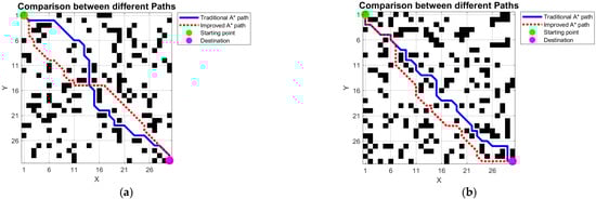
Figure 5. Comparison of typical results of repeated simulation experiments under different obstacle rates: (a) One of the 30 experiments at an obstacle rate of 0.17%; (b) One situation selected from 25 experiments at an obstacle rate of 0.21%; (c) One selected from 20 experiments at an obstacle rate of 0.25%; (d) One selected from 17 experiments at an obstacle rate of 0.29%; (e) One situation selected from 14 experiments at an obstacle rate of 0.33%; (f) One selected from 10 experiments at an obstacle rate of 0.37%.

Table 2. Comparisons of simulation experimental data between traditional A* algorithm and improved A* algorithm.

Obstacle Rate	Algorithm	Execution Time	Path Length	Search Nodes	Turning Points	Energy
0.17%	A*	0.0105	47.46	41	20	73,632.49
	Improved A*	0.0153	45.70	38	17	69,115.08
0.21%	A*	0.0091	52.97	49	29	87,480.14
	Improved A*	0.0067	49.21	44	22	77,357.33
0.25%	A*	0.0003	49.21	44	21	76,564.77
	Improved A*	0.0032	48.04	42	17	71,968.05
0.29%	A*	0.0010	56.97	53	30	93,143.02
	Improved A*	0.0028	56.14	53	26	88,964.10
0.33%	A*	0.0014	55.56	52	23	85,873.18
	Improved A*	0.0050	51.80	47	22	80,505.73
0.37%	A*	0.0009	59.56	56	33	98,669.10
	Improved A*	0.0034	52.73	50	25	84,014.46

Although the improved A* algorithm has a 38% increase in average computation time compared to the traditional A* algorithm, the significant improvement in the path quality proves that the trade-off is reasonable. For the electrically driven heavy-duty six-legged robot in practical applications, energy efficiency and path reliability often take priority over raw computing speed. The additional computation time is mainly attributed to the enhanced heuristic search process, which evaluates multiple candidate paths to optimize smoothness and energy cost. As obstacle density increased, the improved A* algorithm and traditional A* algorithm exhibit a natural decline in performance. However, the improved A* algorithm maintains relatively stable path quality and energy efficiency. The experimental results indicate that the improved A* algorithm has better scalability and environmental adaptability. Therefore, the improved A* algorithm can be applied to complex and dynamic real-world environments.

The experimental results show that the proposed energy consumption model effectively quantifies the energy consumption of the improved A* algorithm and traditional A* algorithm, thereby enabling a clear comparison of their performance. It is achieved by integrating a heuristic cost function into the A* search process. This feature considers the key energy consumption factors, including motor energy consumption, ground friction, turning radius, and load weight, etc.

An error analysis is included to objectively evaluate potential limitations in the simulation experiments. The grid-based discretization method can introduce quantization errors. Continuous terrain features are approximated by discrete cells, which may affect both path smoothness and energy estimation accuracy. Parameters used in the energy consumption model also involve uncertainties. For example, friction coefficients and motor efficiency factors may vary due to experimental conditions or environmental changes. The assumption of static obstacles in offline maps may not fully reflect real-world situations with dynamic elements. It could lead to discrepancies in the robustness of path planning. Additionally, while the Bézier curve smoothing technique improves path continuity, it may cause slight deviations from the geometrically optimal path due to its parametric nature. The limitations are recognized as inherent in simulation-based validation. However, the overall effectiveness of the proposed method will not be compromised. Future work will focus on integrating real-time sensor data and adaptive models to reduce such errors, enhancing practical applicability.

Although the increase in the computing requirements may impose limitations on time critical applications, the future work can optimize the real-time performance of algorithm through parallel computing or heuristic pruning. Overall, the improved A* algorithm achieves a good balance between computational efficiency and path quality, making it highly suitable for applications such as emergency rescue operations in the wild, planetary exploration, and material transportation, all of which prioritize energy efficiency and path smoothness.

5. Conclusions

The electrically driven heavy-duty six-legged robot faces critical challenges in complex terrains, including high energy consumption and stringent smoothness requirements. Therefore, a low-energy path planning method is proposed in this paper based on an improved A* algorithm. The proposed method first establishes energy consumption models for both straight-line walking and turning motions. These models incorporate key influencing factors such as payload, terrain slope, and ground friction coefficients. Building upon the conventional A* algorithm, three key enhancements are introduced to refine the robot’s performances in path planning. The dynamic weight adjustment mechanism is incorporated into the heuristic function, enabling the algorithm to adaptively balance global exploration and local exploitation during the search process. Bézier curve fitting is applied to smooth the generated path, effectively reducing unnecessary turning points and improving trajectory continuity. The nonlinear constraints are integrated to suppress data mutations and outliers, thereby significantly enhancing the robustness and reliability of the algorithm in complex environments.

The three improvement modules in the proposed algorithm do not operate in isolation. They form an organic whole, collectively working towards the ultimate goal of energy consumption minimization. In the early search stage, dynamic weight adjustment assigns a lower weight to the heuristic function. It encourages the algorithm to explore more potential low-energy consumption path regions. Consequently, superior raw material is provided for subsequent smoothing. The nonlinear suppression mechanism ensures stability during the search process. Oscillations caused by heuristic value mutations are avoided. Thus, the regulatory effect of dynamic weight adjustment is allowed to function smoothly. Bézier curve smoothing performs fine-grained geometric optimization on the coarse path generated by the preceding modules. Sharp turns that lead to energy waste are directly eliminated.

The simulation results show that the proposed method consistently generates shorter and smoother paths in environments with different obstacle rates. Specifically, it achieves a 7.2% reduction in average path length, a 25.9% decrease in the number of turning points, and a 5.75% reduction in average energy consumption. The improvements significantly enhance both the navigational feasibility and the energy efficiency of paths, which offers an effective planning strategy to support extended operational endurance for electrically driven heavy-duty six-legged robot.

A fundamental distinction is examined between the proposed energy-optimal method and algorithms that prioritize solely the shortest geometric path. While the comparative methods demonstrate excellence in minimizing distance, they frequently generate paths characterized by numerous turns. Such paths prove highly energy-inefficient for heavy-duty legged robots, as confirmed by comparative results. Studies focusing on computational speed and search efficiency enhancements are additionally addressed. Their contributions are acknowledged, but their performance metrics typically fail to incorporate the physical energy cost for specific robotic platforms. The critical gap is bridged through the direct integration of an energy consumption model into the planning process. The Bézier curve-based smoothing technique employed here is explicitly guided by an energy consumption model. This approach is contrasted with general-purpose smoothing methods. Emphasis is placed on optimizing energy-efficient smoothness, which effectively reduces acceleration/deceleration cycles and aggressive turns rather than focusing exclusively on geometric smoothness.

It should be noted that the current research in this paper is primarily validated through simulation. Although the proposed algorithm has shown promising performance in simulated environments, its effectiveness and stability in real-world scenarios need further verification. Based on the developed prototype of the electrically driven heavy-duty six-legged robot, the next step is to evaluate the practical applicability and robustness of the proposed improved A* algorithm under realistic conditions.

References

- Liu, L.; Wang, X.; Yang, X.; Liu, H. Path planning techniques for mobile robots: Review and prospect. Expert Syst. Appl. 2023, 227, 120254. [Google Scholar] [CrossRef]
- Raj, R.; Kos, A. A comprehensive study of mobile robot: History, developments, applications, and future research perspectives. Appl. Sci. 2022, 12, 6951. [Google Scholar] [CrossRef]
- Moniruzzaman, M.D.; Rassau, A.; Chai, D.; Islam, S.M.S. Teleoperation methods and enhancement techniques for mobile robots: A comprehensive survey. Robot. Auton. Syst. 2022, 150, 103973. [Google Scholar] [CrossRef]
- Zhuang, H.; Wang, N.; Gao, H.; Deng, Z. Power consumption characteristics research on mobile system of electrically driven large-load-ratio six-legged robot. Chin. J. Mech. Eng. 2023, 36, 26. [Google Scholar] [CrossRef]
- Xu, P.; Ding, L.; Li, Z.; Yang, H.; Wang, Z.; Gao, H.; Zhou, R.; Su, Y.; Deng, Z.; Huang, Y. Learning physical characteristics like animals for legged robots. Nat. Sci. Rev. 2023, 10, nwad045. [Google Scholar] [CrossRef]
- Zhuang, H.; Wang, J.; Wang, N.; Li, W.; Li, N.; Li, B.; Dong, L. A review of foot-terrain interaction mechanics for heavy-duty legged robots. Appl. Sci. 2024, 14, 6541. [Google Scholar] [CrossRef]
- Xi, D.; Gao, F. Type synthesis of walking robot legs. Chin. J. Mech. Eng. 2018, 31, 15. [Google Scholar] [CrossRef]
- Hwang, J.Y.; Kim, J.S.; Lim, S.S.; Park, K.H. A fast path planning by path graph optimization. IEEE Trans. Syst. Man Cybern. A Syst. Hum. 2003, 33, 121–129. [Google Scholar] [CrossRef]
- Alshammrei, S.; Boubaker, S.; Kolsi, L. Improved Dijkstra algorithm for mobile robot path planning and obstacle avoidance. Comput. Mater. Contin. 2022, 72, 5939–5954. [Google Scholar] [CrossRef]
- Zhou, Y.; Huang, N. Airport AGV path optimization model based on ant colony algorithm to optimize Dijkstra algorithm in urban systems. Sustain. Comput. Inform. Syst. 2022, 35, 100716. [Google Scholar] [CrossRef]
- Sundarraj, S.; Reddy, R.V.K.; Basam, M.B.; Kumar, M.S.; Rajesh, M. Route planning for an autonomous robotic vehicle employing a weight-controlled particle swarm-optimized Dijkstra algorithm. IEEE Access 2023, 11, 92433–92442. [Google Scholar] [CrossRef]
- Noreen, I.; Khan, A.; Habib, Z. A comparison of RRT, RRT* and RRT*-smart path planning algorithms. Int. J. Comput. Sci. Netw. Secur. 2016, 16, 20–27. [Google Scholar]
- Zhang, H.; Wang, Y.; Zheng, J.; Yu, J. Path planning of industrial robot based on improved RRT algorithm in complex environments. IEEE Access 2018, 6, 53296–53306. [Google Scholar] [CrossRef]
- Maurović, I.; Seder, M.; Lenac, K.; Petrović, I. Path planning for active SLAM based on the D* algorithm with negative edge weights. IEEE Trans. Syst. Man Cybern. Syst. 2017, 48, 1321–1331. [Google Scholar] [CrossRef]
- Yang, H.; Teng, X. Mobile robot path planning based on enhanced dynamic window approach and improved A* algorithm. J. Robot. 2022, 2022, 2183229. [Google Scholar] [CrossRef]
- Xiang, D.; Lin, H.; Ouyang, J.; Huang, W. Combined improved A* and greedy algorithm for path planning of multi-objective mobile robot. Sci. Rep. 2022, 12, 13273. [Google Scholar] [CrossRef]
- Liu, Z.; Liu, H.; Lu, Z.; Zhong, H.; Zhang, T. A dynamic fusion pathfinding algorithm using delaunay triangulation and improved A-star for mobile robots. IEEE Access 2021, 9, 20602–20621. [Google Scholar] [CrossRef]
- Zhuang, H.; Dong, K.; Qi, Y.; Wang, N.; Dong, L. Multi-destination path planning method research of mobile robots based on goal of passing through the fewest obstacles. Appl. Sci. 2021, 11, 7378. [Google Scholar] [CrossRef]
- Xu, P.; Ding, L.; Wang, Z.; Gao, H.; Deng, Z.; Huang, Y. Contact sequence planning for six-legged robots in sparse foothold environment based on Monte-Carlo tree. IEEE Robot. Autom. Lett. 2021, 7, 826–833. [Google Scholar] [CrossRef]
- Liu, S.; Sun, D. Minimizing energy consumption of wheeled mobile robots via optimal motion planning. IEEE/ASME Trans. Mechatron. 2013, 19, 401–411. [Google Scholar] [CrossRef]
- Yao, M.; Deng, H.; Feng, X.; Li, Y.; Zhang, T. Improved dynamic windows approach based on energy consumption management and fuzzy logic control for local path planning of mobile robots. Comput. Ind. Eng. 2024, 187, 109767. [Google Scholar] [CrossRef]
- Wang, X.; Cao, J.; Cao, Y.; Zhang, J.; Chen, X. Energy-efficient trajectory planning for a class of industrial robots using parallel deep reinforcement learning. Nonlinear Dyn. 2025, 113, 8491–8511. [Google Scholar] [CrossRef]
- Soijoyo, S.; Wardoyo, R. Wireless sensor network energy efficiency with fuzzy improved heuristic A-Star method. Int. J. Adv. Comput. Sci. Appl. 2017, 8, 341–348. [Google Scholar] [CrossRef]
- Wang, Z.; Gao, F.; Zhao, Y.; Yin, Y.; Wang, L. Improved A* algorithm and model predictive control-based path planning and tracking framework for hexapod robots. Ind. Robot. 2023, 50, 135–144. [Google Scholar] [CrossRef]
- Chen, L.; Wang, Q.; Deng, C.; Xie, B.; Tuo, X.; Jiang, G. Improved Double Deep Q-Network Algorithm Applied to Multi-Dimensional Environment Path Planning of Hexapod Robots. Sensors 2024, 24, 2061. [Google Scholar] [CrossRef]
- Wang, G.; Ding, L.; Gao, H.; Deng, Z.; Liu, Z.; Yu, H. Minimizing the energy consumption for a hexapod robot based on optimal force distribution. IEEE Access 2020, 8, 5393–5406. [Google Scholar] [CrossRef]
- Yang, K.; Liu, X.; Liu, C.; Wang, Z. Motion-Control Strategy for a Heavy-Duty Transport Hexapod Robot on Rugged Agricultural Terrains. Agriculture 2023, 13, 2131. [Google Scholar] [CrossRef]
- Hu, Y.; Guo, W.; Lin, R. An Investigation on the Effect of Actuation Pattern on the Power Consumption of Legged Robots for Extraterrestrial Exploration. IEEE Trans. Robot. 2023, 39, 923–940. [Google Scholar] [CrossRef]
Disclaimer/Publisher’s Note: The statements, opinions and data contained in all publications are solely those of the individual author(s) and contributor(s) and not of MDPI and/or the editor(s). MDPI and/or the editor(s) disclaim responsibility for any injury to people or property resulting from any ideas, methods, instructions or products referred to in the content. |
© 2025 by the authors. Licensee MDPI, Basel, Switzerland. This article is an open access article distributed under the terms and conditions of the Creative Commons Attribution (CC BY) license (https://creativecommons.org/licenses/by/4.0/).