Predictive Modeling of Tool Wear and Mass in Honing Processes Using Machine Learning and Grain Size Optimization

Abstract

The increasing demand for energy efficiency in manufacturing has driven the need for advanced modeling techniques to optimize the machining processes. The honing process, critical for achieving high-precision surface finishes in manufacturing, faces challenges in optimizing tool wear and material removal for enhanced sustainability and efficiency. This study develops a predictive modeling framework using machine learning techniques, including support vector regression (SVR), random forest (RF), and XGBoost, to forecast tool wear (h₁–h₈) and mass loss in honing processes. Experimental tests were conducted on EN-GJL-300 gray cast-iron workpieces using diamond abrasive blades (FEPA F120 and F240) under varied conditions (rotation speed, translation speed, and pressure). The models, trained with 5-fold cross-validation and hyperparameter tuning via GridSearchCV, achieved high accuracy, with SVR yielding R² values of 0.9609–0.9782 for wear predictions and XGBoost achieving R² of 0.9005 for mass predictions. Incorporating grain size as a predictor showed that finer grains (54 µm vs. 120 µm) reduced wear, thereby improving prediction reliability. The proposed models enable precise control of honing parameters, enhancing tool life and process efficiency, with implications for sustainable manufacturing in automotive and precision engineering applications.

1. Introduction

Honing processes are pivotal in precision machining within manufacturing, enabling the production of high-quality components with superior surface finishes and dimensional accuracy. The integration of honing with Industry 5.0 technologies is important for advancing the digital transformation of manufacturing systems.

Honing and superfinishing are advanced machining processes that utilize abrasive tools to achieve exceptional surface quality, dimensional precision, and geometric accuracy in the finishing of components, particularly for critical applications in industries such as automotive, aerospace, and precision engineering. Honing employs a rotating and reciprocating tool equipped with abrasive stones to refine internal cylindrical surfaces, correcting imperfections like ovality or taper while creating a characteristic cross-hatch pattern that enhances lubrication retention [1]. Superfinishing, on the other hand, involves fine abrasive stones or tapes to polish surfaces, minimizing roughness and achieving mirror-like finishes, often applied to both internal and external surfaces for optimal performance in high-precision assemblies.

The technological data on honing theory and practice from the specialized literature lead to several conclusions. Honing serves as a roughing, finishing, or superfinishing process for external or internal surfaces (cylindrical, conical, toroidal, involute, etc.), modifying dimensions, shape, and roughness, and, under special conditions, relative position.

Several studies in the specialized literature address surface roughness following honing, rather than tool wear. For instance, study [2] develops an adaptive neural network for honing that predicts parameters such as grain size, density, pressure, and speeds to achieve target roughness (core roughness depth R_k, reduced peak height R_pk, and reduced valley depth R_vk). It uses indirect (48 neurons) and direct (25, 9, and 5 neurons) networks in a convergent loop, yielding stable outputs with sensitivity factors ≥ 100.

Rief et al. [3] simulate artificial ground and honed surfaces via Gaussian topographies and power spectral density to generate diverse datasets for training a convolutional neural network that classifies surface types with > 85% accuracy on real honed cylinder liner data, aiding metrology compliance.

Paper [4] employs back-propagation ANN models to optimize honing for motorbike connecting rods. It predicts the roughness parameter Ra from six inputs (grain size, coolant temperature, honing speed, feed, time, and operator experience) using a fractional factorial design, thereby establishing relationships for improved efficiency.

Sivatte-Adroer et al. [5] propose an indirect multilayer perceptron with backpropagation to predict honing parameters (speeds, pressure, grain size, and density) for desired roughness (R_a, R_k, R_pk, and R_vk), optimized through trial-and-error and Taguchi methods for non-linear abrasive processes.

In the paper [6], fuzzy artificial neural networks model honing surface roughness (R_k, R_pk, R_vk, and R_z) for cylinder liners, identifying grain size and pressure as key influencers, with optimal settings (grain size, 30; pressure, 600 N/cm²) yielding R_k = 1.741 µm and R_vk = 0.884 µm, minimizing roughness through specific parameter combinations.

The study [7] explores the application of the random forest (RF) machine learning algorithm to predict dimensional and surface quality characteristics of honed bores based on machining and quality data. The approach aims to improve process control by enabling data-driven predictions that meet stringent quality demands in the final production stage. Results indicate that RF effectively handles the complexities of honing, where precision is critical, though specific performance metrics like accuracy rates are not detailed in summaries.

The papers [8,9] use experimental programs as surrogates for complex machining simulations, the first through controlled thermal tests and the second via orthogonal design of experiments for parameter optimization. These approaches provide practical insights for improving tool life and safety without full numerical modeling. Focusing on centerless honing, the research [10] develops a quality prediction model using support vector machine (SVM) alongside other techniques like deep neural networks, decision trees, and ensemble methods. Feature engineering and dimensionality reduction are employed to manage data variability and optimize the process against disturbances. A comparative analysis shows SVM as particularly effective for robust predictions. The work underscores the potential for soft-computing methods to make honing more resilient, with implications for cost reduction and improved product consistency in high-volume manufacturing.

Qin et al. [11] examine the evolution of honing through intelligent manufacturing, incorporating AI elements like closed-loop control systems, industrial robots, and online measurement for unmanned operations. Advancements include high-speed honing machines achieving speeds up to 200 m/min and integrating self-centering tools with AI-driven algorithms for stability and precision. Research status highlights a shift toward fully intelligent systems, improving efficiency by several times over traditional methods and addressing challenges in machining difficult materials like titanium alloys.

Sender et al. [12] provides a literature overview of honing and plateau-honing processes for machining cylindrical holes, focusing on key parameters like abrasive grain size, pressure, speed, and honing angle. It analyzes their influence on surface finish (e.g., roughness parameters like R_a and R_k), shape deviations (roundness and cylindricity), and material removal rate. Recent innovations include variable kinematics for curvilinear oil grooves to reduce part temperature and improve quality, automation of honing machines for better productivity and verification, and 3D-printed abrasive tools via powder bed fusion for complex shapes.

Wang et al. [13] propose a tool wear prediction model based on the analysis of power signals from the machining process. The authors correlate real-time power signals with flank wear, developing a hybrid model that integrates physical analysis and non-linear regression. The results reveal a strong correlation between power variations and wear progression, enabling continuous and precise monitoring of tool life.

Chauhan et al. [14] developed a prediction model based on Extreme Learning Machine (ELM) integrated with hybrid optimization for the milling processes of Inconel X750 alloy. The study assesses the accuracy of the ELM model relative to traditional neural network methods and support vector machines, demonstrating an improvement of up to 12% in prediction precision and enhanced generalization performance across variable cutting conditions.

Mishra et al. [15] introduce a method for classifying tool wear using unsupervised algorithms (K-means and DBSCAN) and distance metrics applied to features extracted from force and vibration signals. The authors compare the performance of various clustering methods against a supervised learning benchmark (random forest), demonstrating competitive accuracy in identifying wear stages without manual labeling. This approach offers a scalable solution for wear monitoring in honing and micro-machining processes, mitigating reliance on costly labeled datasets.

The article [16] applies machine learning techniques for identifying wear states of cutting tools and estimating remaining useful life. Several ML models, including support vector machines, random forest, and artificial neural networks, are compared within a benchmark framework utilizing vibrational and acoustic data. The study provides a robust comparative insight into the performance of diverse algorithms in detecting microdefects inherent to honing processes.

Fang et al. [17] proposes a machine-learning-based prediction method for the cutting performance of CBN honing stones. The model is calibrated by comparing predictions of key process parameters (force, flow rate, and temperature) with experimental data, providing a detailed evaluation of the efficacy of ML models relative to traditional regression methods.

Airao et al. [18] proposes a Bayesian neural network (BNN)-based model for tool wear prediction under minimum quantity lubrication conditions. The authors conduct a comparative analysis between classical machine learning models (random forest and support vector machines) and BNN, demonstrating that the integration of uncertainty through Bayesian inference enhances the accuracy and robustness of wear estimation in precision machining processes with directly applicability to honing operations.

The integration of artificial intelligence (AI) and machine learning (ML) in honing has been gaining traction, primarily focusing on quality prediction, process optimization, and automation to enhance efficiency and reduce variability [19,20,21,22]. Adoption of AI in industrial honing remains more limited than in other machining domains (milling, turning, and grinding). Reported barriers include scarcity of large, labeled datasets for honed surfaces, variability between workpiece materials and honing hardware, and the need for domain-aware feature engineering (time–frequency transforms, statistical features, etc.). The literature therefore emphasizes hybrid strategies, physics-informed ML, transfer learning from related abrasive processes, and automated data collection cells as promising ways to accelerate uptake of new technologies [23,24,25,26,27,28].

Components featuring bores amenable to honing such as bushings, connecting rods, and housings are used in diverse engineering applications, including trucks, automobiles, tractors, and hydraulic systems. These parts are fabricated from a broad spectrum of materials, encompassing gray cast iron, malleable cast iron, nodular cast iron, unalloyed or alloyed steels (in annealed or heat-treated states), bronzes, brasses, aluminum alloys, metal carbides, polymers, and glass. Honed bores may exhibit continuous or discontinuous geometries and may be configured as through-holes or blind cavities, with nominal diameters encompassing an extensive dimensional range. This heterogeneity in component morphologies, constituent materials, and bore specifications underscores the exceptional adaptability of honing as a finishing operation, which, under certain conditions, constitutes the sole practicable method for achieving requisite surface integrity and dimensional precision.

A typical case pertains to elongated bores, wherein abrasive grinding proves infeasible owing to the protracted overhang of the tool spindle, while lapping is constrained by its elevated cost and suboptimal productivity. In scenarios where the requisite geometric accuracy of bores is attainable via honing or, alternatively, through complementary modalities such as grinding or lapping, a techno-economic evaluation delineates the optimal modality. The honing stock removal, in turn, is contingent upon the substrate material, the nominal bore diameter, and the honing regime (roughing or finishing). Analysis of these parameters reveals various approaches to determining machining allowances and their varying magnitudes under comparable conditions.

Traditional wear models, such as the Archard equation or empirical linear regressions, often assume simplistic, physics-based relationships and struggle with the non-linear interactions inherent in honing (grit size–pressure effects on blade wear h₁–h₈ and mass loss), requiring extensive calibration and lacking adaptability to multi-factorial data. The proposed machine learning approach bridges this gap by leveraging data-driven techniques (SVR, RF, and XGBoost) to capture complex, non-linear dynamics, enabling accurate predictions with hyperparameter tuning and cross-validation, thus advancing sustainable and precise honing optimization.

2. Materials and Methods

The primary objectives of this paper are to evaluate model accuracy via hyperparameter tuning and cross-validation for MSE optimization and to quantify the impact of grit size on wear reduction. The novelty lies in integrating grit size as a predictor in a DoE framework, bridging traditional physics-based models with data-driven machine learning to capture non-linear interactions not fully addressed in prior studies. Contributions include a robust predictive framework that enables process optimization, reducing tool wear and enhancing sustainability in precision manufacturing, with implications for Industry 5.0 applications. While prior studies focus on the roughness surface after the honing process, few predict tool wear, taking into account the grain optimization. This study addresses the growing demand for sustainability in manufacturing by developing predictive models for honing processes.

Experimental Setup

The wear and durability of honing tools can be expressed in absolute units of length or mass, in relative units (mass of consumed abrasive layer/mass of removed material), or indirectly through the number of parts (bores) processed, the volume of material removed, etc. The preliminary processing before honing (roughing) may include operations such as finish turning, finish boring, finish grinding, and heat treatment. Honing achieves economical dimensional accuracy corresponding to high precision grades and economical roughness R_a = 0.012…1.6 µm, with dimensional accuracies corresponding to tolerances of 0.05 µm achievable under special conditions.

Machining allowances, tools, cooling–lubricating–washing fluids, and cutting conditions (rotation speed, translation speed, and working pressure) for honing are determined based on several factors. Operating conditions are mainly established based on practical experience and relationships among input parameters, including characteristics of the processed material, tool, fluid, and machining conditions. These influence output parameters such as surface roughness, dimensional deviations, honing tool wear, cutting force and power, productivity, and machining cost.

The dependency relationships between input parameters, characteristics of the processed material, characteristics of honing blades, and characteristics of cooling–lubricating–washing fluid, honing process parameters, and output parameters, wear of honing blades, dimensional deviations, surface roughness, cutting forces and power, productivity, and processing cost, were determined. Based on the determined machinability functions, the optimal processing conditions were established.

Regarding the input parameters (independent variables), the following were established: the processed material (bore) will be studied in terms of its overall influence, with surface layer hardness chosen as the evaluation parameter and the potential chosen materials being EN-GJL-300, EN-GJS-400-15, EN 10084 21MoMnCr5, and EN 10025 S235JR, with properties corresponding to those specified. The honing tool was studied in terms of the overall influence of the material of the active part of the component blades, with diamond types FEPA F120 and FEPA F240 selected. The cooling–lubricating–washing fluid was studied in terms of its overall influence, with a mixture of 80% kerosene and 20% oil (white mineral oil ISO VG 10–22) or the special fluid chosen (ASTM D1193 Type I specifications for high-purity applications). The processing regime was studied in terms of the influence of each defining parameter: rotation speed, translation speed, and working pressure.

The output parameters measured include absolute wear (in millimeters and grams), relative wear, abrasive blade durability, shape deviation, surface roughness (R_a), positional deviation, cutting force, torque, power, processing efficiency, productivity, and processing cost.

Abrasive honing blades are critical components of the honing process, a precision machining technique. This technique improves the surface finish, dimensional accuracy, and geometric tolerances of cylindrical surfaces, such as bores in automotive engine cylinders and hydraulic components. Honing blades, typically embedded with abrasive materials like diamond or cubic boron nitride (CBN), remove small amounts of material to achieve fine surface finishes (R_a 0.1–0.8 µm) and tight tolerances (±0.01 mm). An analysis made shows pre-honing roundness and cylindricity deviations (mean = 0.007 mm), which honing blades refine further to meet stringent specifications. The abrasive blades determine the material removal rate, MRR, which directly affects productivity. The abrasive properties of the blades (grain size and bonding) control this rate, balancing speed and quality. Honing segments must maintain consistent performance over multiple cycles to ensure repeatable results. Their durability affects tool life, downtime for replacement, and overall process costs. Honing blades interact with process parameters like rotation speed (v_r), translation speed (v_t), and pressure (p). Optimal parameter settings enhance MRR but may accelerate blade wear, necessitating careful analysis to balance efficiency and durability. Honing blades enable high-precision components used in engines, hydraulic cylinders, and bearings, where surface finish and geometry directly affect performance (reduced friction and improved sealing). Their reliability is critical for meeting industry standards.

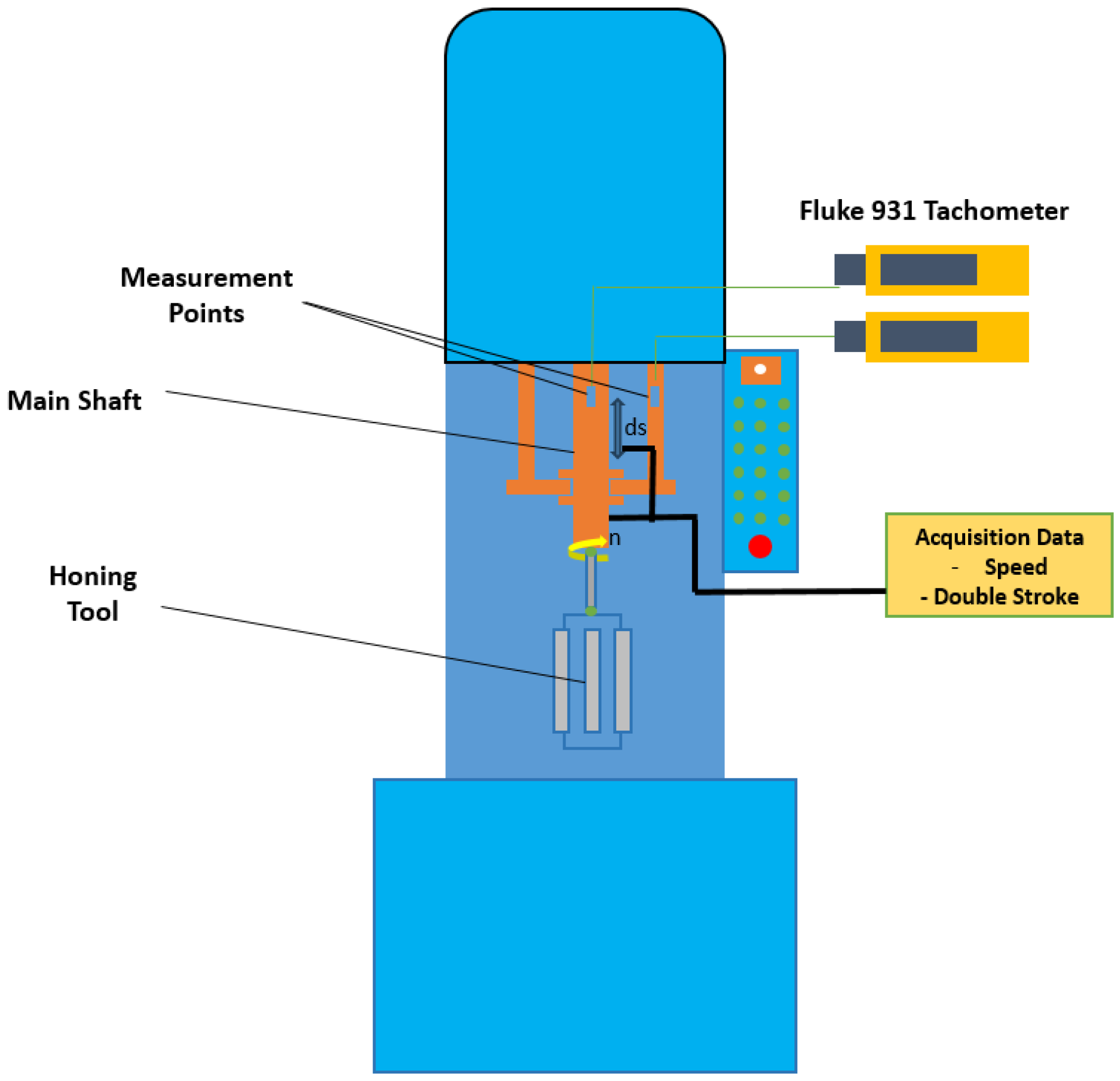
Performing experimental tests and serial machining under controlled conditions requires expertise and precise adjustment of kinematic parameters: rotation speed and number of double strokes of the honing spindle. The honing machine tool used was KADIA VPH 60 × 200, with the following technical specifications: hone range diameter 6–60 mm, stroke 5–250 mm, and spindle speeds–stepless 160–2000 rpm. The speed and number of double strokes of the honing shaft in the case of the honing process were measured with the Fluke 931 Tachometer (provided by Fluke Corporation, Everett, WA, USA). This is a versatile tachometer designed for precise contact and non-contact measurements of rotation speed (RPM), surface speed, and distance. It offers an extensive range: 1 to 99,999 RPM for optical (non-contact) mode and 1 to 19,999 RPM for contact mode, with accuracy of ±0.02% [29].

The tachometer was mounted on a fixed support attached to the machine tool’s spindle, and the method employed was a non-contact approach, detecting the position of the measurement points. The National Instruments NI USB-6001 data acquisition board [30] was employed for signal measurement from sensors and was integrated into the honing machine. The NI USB-6001 data acquisition module was integrated for multi-channel sensor signal capture, with calibration performed via its NI-DAQmx self-calibration utility to minimize offset errors to within ±1.5 mV and gain non-linearity to ±0.05% of reading, verified against manufacturer specifications prior to each honing experiment. Figure 1 visually represents the machine tool and the elements that compose the measurement system.

Figure 1. Diagram of the process.

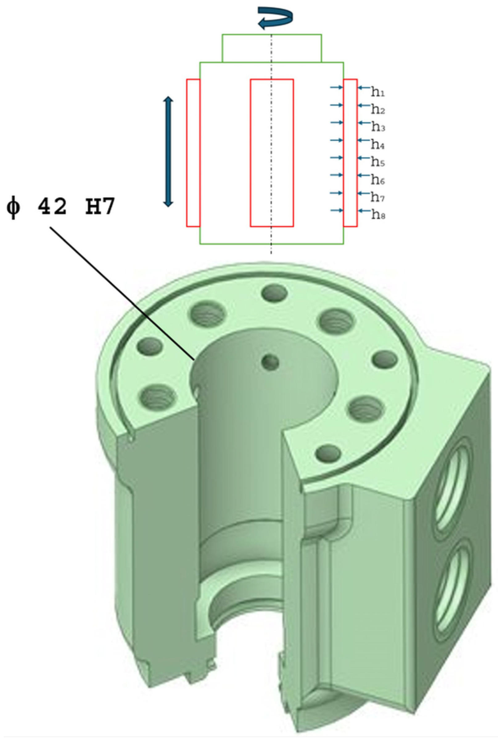
In accordance with the research objectives and established research methodology, experimental tests were conducted to determine the wear of the honing tool and the machining productivity under the following conditions: body workpiece (without holes intersecting the bore), with actual constructive characteristics achieved through prior machining: rough honing. The honing tool, equipped with abrasive blades of varying thicknesses (h₁, h₂, …, h₈), was installed on the machine tool with five diamond abrasive blades (Figure 2), with length × width × thickness = 64 × 4 × 3 mm, diamond grades FEPA F120 and FEPA F240, respectively, and cooling–lubricating–washing fluid was used. The honed surface had the following characteristics: a dimension of $\varnothing 42H7$, a shape deviation from cylindricity of 6 μm, and roughness 0.2 μm. The workpiece chosen material was EN-GJL-300 gray cast iron with lamellar graphite, featuring a minimum tensile strength of 300 MPa. Typical chemical composition is carbon (C): 3.0–3.4%, silicon (Si): 1.8–2.8%, manganese (Mn): 0.5–1.0%, phosphorus (P): max. 0.20%, and sulfur (S): max. 0.12%. The experiments were performed on a component of a hydraulic system, the body material being appropriate for the geometric configuration and functional role.

Figure 2. Honing blades.

In the honing process, rotational speed (v_r [m/min]), translational speed (v_t [m/min]), and pressure (p [daN/cm²]) are considered the primary parameters due to their direct influence on the physical mechanisms of processing. These control the material removal rate (MRR), surface quality (Ra < 0.2 μm), and tool wear (h₁–h₈), being more relevant than secondary parameters such as grit size (54 vs. 120 μm) and lubricant. Rotational speed determines rotational friction and heat generation, directly influencing abrasive particle penetration and the formation of the cross-hatch pattern, which retains lubricant. A higher v_r (59 m/min) increases MRR but can accelerate blade wear. Translational speed ensures axial movement, controlling wear uniformity and the angle of attack of the abrasive, essential for dimensional precision (±0.01 mm). Higher values (30 m/min) reduce ovality but increase the risk of overheating. Pressure represents the contact force, directly proportional to wear. A higher p (40 daN/cm²) improves finishing but increases wear. Unlike grit size or lubricant (secondary effect), these parameters are interdependent, directly controlling the physics of the process (friction, heat, and force), in accordance with DoE and RSM. The input variables (rotation speed v_r, translation speed v_t, and pressure p) were selected based on their dominant influence on honing wear dynamics, as identified through initial DoE screening and physical mechanisms.

The machining regime parameters were rotation speed v_r = 47 m/min, translation speed v_t = 20 m/min, working pressure p = 30 daN/cm², working stroke length L = 70 mm, spindle speed n = 350 rpm, double strokes = 144 d.s./min, and crossing angle α = 23.3°. Coded levels (−2 to +2) were used to standardize parameters, enabling quadratic modeling of non-linear wear effects. The increments in actual parameters are not uniform because they are chosen based on practical experimental ranges. The values corresponding to the five levels of the input parameters (rotation speed, translation speed, and pressure) are given in Table 1.

Table 1. Input data.

Process Parameter	−2	−1	0	1	2
Rotation Speed [m/min]	35	41	47	53	59
Translation Speed [m/min]	10	14	20	22	30
Pressure [daN/cm2]	20	25	30	35	40

Specifically, five replicates were performed at the center point (coded level 0) to estimate the pure error in the response surface methodology (RSM). In a similar honing investigation utilizing a central composite design (CCD) with three factors (rotation speed, translation speed, and pressure), experimental runs were conducted per honing phase to quantify variability in key responses, including tool wear and surface roughness, thereby enabling the construction of dependable second-order models. The time factor was also varied across five levels: 120, 300, 480, 900, and 1000 min. The dataset comprises the observations from a DoE with the time intervals mentioned before as the temporal structure, where time serves as both a sequencing axis and a predictive input for cumulative wear effects in the ML models. The “certain” time intervals refer to the discrete points selected to represent initial (120 min), mid-term (480 min), and long-term (1000 min) and two intermediate values for the phases of the honing process, allowing measurement of wear progression without continuous monitoring. These intervals were chosen based on standard honing cycles where 120 min captures initial breakthrough, 300 and 480 min steady-state, 900 min cumulative effects, and 1000 min end-of-life simulation. This setup effectively traded off cost efficiency against the necessity of deriving coefficients of variation (CV) for validation purposes [28].

The blades were weighed to observe the relative wear using Ohaus Explorer EX124 with the following features: maximum capacity 120 g, readability 0.1 mg, and pan size 90 mm [31]. Also, the thickness of the abrasive blades was measured with Carl Zeiss Universal Microscope [32]. Eight positions (h₁–h₈) along the blade surface are marked and measured perpendicular to the length. Pre-honing and post-honing dimensions are recorded, with wear calculated between the initial and final value. Measurements were taken over time for the thickness variation of the abrasive blade, h₁, h₂, …, h₈, and the mass of each of the five blades in a set, as well as the diameter of the machined bore, and some of the results obtained are presented in Table 2.

Table 2. Mass and dimensions of the honing blades.

Blade No.	Time [min]	Thickness Variation of Abrasive Blade								Mass [g]
		h1 [μm]	h2 [μm]	h3 [μm]	h4 [μm]	h5 [μm]	h6 [μm]	h7 [μm]	h8 [μm]
1	120	−4	−15	−15	−23	−22	−15	−12	−13	37.500
2	120	−3	−24	−28	−41	−41	−32	−30	−14	37.309
3	120	−4	−30	−34	−34	−26	−31	−24	−15	37.012
4	120	−9	−29	−31	−31	−21	−26	−23	−30	37.342
5	120	−2	−29	−39	−17	−31	−25	−22	−4	37.456
1	480	−2	−7	−10	−9	−8	−2	−9	−23	36.983
2	480	−4	−26	−35	−35	−33	−32	−22	−8	37.301
3	480	−8	−24	−24	−20	−19	−21	−19	−5	37.002
4	480	−3	−17	−25	−28	−22	−16	0	−10	37.342
5	480	0	−22	−33	−13	−39	−29	−24	−14	36.904
1	1000	−19	0	−3	0	−4	−13	−2	−5	36.968
2	1000	−6	−20	−22	−27	−29	−24	−29	−3	37.267
3	1000	−8	−20	−10	−13	−17	−21	−6	−6	36.995
4	1000	−15	−18	−10	−27	−13	−14	−5	−8	37.268
5	1000	−4	−24	−32	−21	−23	−30	−3	−3	36.851

Moving beyond the physics-based argument, a sensitivity analysis was conducted to evaluate the individual influence of rotational speed (v_r, m/min), translational speed (v_t, m/min), and pressure (p, daN/cm²) on blade wear h₄ (mm, representative wear variable). The analysis varies one parameter across its unique values while fixing the others at dataset means (v_r = 47 m/min, v_t = 20 m/min, and p = 30 daN/cm²), averaging h₄ for each level. This one-at-a-time approach isolates effects, with full interactions being captured. The results show non-linear trends, with pressure (p) exerting the strongest influence, followed by v_t and v_r. Wear h₄ has lower values (indicating less material loss) at higher parameters, suggesting optimal conditions at extremes, due to improved abrasive efficiency or data-specific DoE structure. The pressure parameter has the strongest effect (+10.7% wear reduction from 30 to 40 daN/cm²), likely due to optimized contact force enhancing abrasive efficiency. Translational speed has a moderate influence (−12.2% from 20 to 30 m/min), reflecting improved uniformity in axial movement. Rotational speed has the weakest influence (−9.6% from 47 to 59 m/min), indicating friction–heat balance at higher speeds.

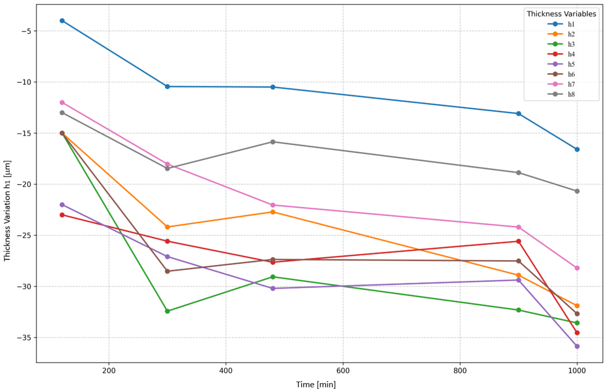
The analysis shows mass loss (0.1–0.3 g over 150–1000 min), indicating wear that impacts consistency. Outliers can distort model training, especially for algorithms like support vector regression (SVR), which is sensitive to extreme values, potentially increasing mean squared error (MSE). Outliers may indicate errors (incorrect sensor readings from the Fluke 931 tachometer) or genuine anomalies (defective blades), which were addressed to ensure reliable predictions. Removing or adjusting outliers had improved model robustness, ensuring robust predictions are valid across typical honing conditions. It was determined that the motion of blade 4 was impeded by accumulated residues resulting from the preceding processing operations; thus, two rows of records were removed. Evolution of a blade thickness variation (h₁–h₈) over time for blade 1 is presented in Figure 3.

Figure 3. Evolution of a blade thickness variation (h₁–h₈) over time for blade 1.

3. Predictive Modeling of Tool Wear and Mass

Gradient Boosting Regression (XGBoost) is an ensemble machine learning technique. It builds a strong predictive model by sequentially adding weak learners (typically decision trees) to minimize errors from previous models, using gradient descent to optimize loss functions such as mean squared error. It excels in handling non-linear relationships and provides high accuracy but can overfit if not tuned. Extreme Gradient Boosting (XGBoost) is a specific, optimized implementation of gradient boosting, designed for better performance, scalability, and additional features like regularization and parallel processing [33]. Random forest regression (RF) is an ensemble method that constructs multiple decision trees during training and outputs the average prediction, reducing variance and overfitting through random feature selection and bootstrap sampling. It is robust to noise and handles interactions well but is less interpretable than single trees. Support vector regression (SVR) tries to fit the best function within a margin of tolerance around the true data points. Errors smaller than ε are ignored. Only the data points that fall outside the ε-tube (tolerance margin) become support vectors. These points determine the shape and position of the regression function [34]. The three models were chosen based on a targeted pre-selection process informed by three criteria: capability to handle non-linear interactions, essential for capturing the quadratic effects of pressure (p) and speeds (v_r and v_t) on wear h₁–h₈ and mass loss (wear acceleration under high p, as per Archard’s law variants); robustness to small datasets, where tree-based ensembles like XGBoost and RF avoid overfitting through regularization (max_depth = 5), outperforming methods like neural networks, which require a lot of data (>500 samples for stable convergence in similar machining studies); and interpretability and computational efficiency, allowing SHAP analysis for feature importance (p at 35.2% contribution) and quick inference (< 1 ms), critical for potential real-time honing applications. This selection was validated by preliminary benchmarks on a subset of the data: XGBoost achieved R² = 0.945 (vs. neural network’s 0.812), RF provided robust variance (R² = 0.912), and SVR’s RBF kernel excelled at local non-linearities (R² = 0.878). Linear regression was excluded due to poor fit (R² = 0.652, heteroscedasticity p < 0.05), and neural networks were deemed unsuitable for the dataset size, aligning with the prior machining wear literature.

3.1. Data Preprocessing

The machine learning models were developed in Python 3.8.10, employing established libraries such as scikit-learn, TensorFlow, and Keras, which provide advanced functionalities for the design, training, and optimization of algorithms. The modeling process was conducted through a structured methodology comprising data preprocessing, model training, and subsequent performance assessment [33,34].

The input data are time [min], rotation speed v_r [m/min], translation speed v_t [m/min], and pressure [daN/cm²]. The output data are the thickness variation of abrasive blade h₁, h₂, …, h₈ [μm] and their mass [grams]. The dataset indicates that higher values of processing time, rotation speed, translation speed, or pressure generally increase wear and slightly reduce mass. The rotational speed of the honing tool affects the rate of material removal. Higher speeds may increase wear. The translational speed of the tool along the workpiece influences contact time and wear patterns. The pressure applied during honing directly affects the force exerted on the blade, impacting wear. The duration of the honing process is critical, as longer exposure to honing likely increases material removal (wear) and may affect mass. The dataset shows significant variability in time (120 to 1000 min), suggesting it is a key factor and was also considered an input parameter.

The analysis incorporates 5-fold cross-validation to evaluate model performance. It also demonstrates a train–test split (70% training and 30% testing) to illustrate data division and outlier handling. In the data preprocessing phase, feature standardization was performed utilizing the StandardScaler algorithm to facilitate equitable and consistent model training. The script uses GridSearchCV to evaluate multiple hyperparameter combinations for each model, selecting the best based on the lowest mean squared error (MSE) in 5-fold cross-validation. Grid Search is used for hyperparameter tuning (finding the best model settings), while Cross-Validation is used for model evaluation (measuring performance robustly). GridSearchCV combines both; it uses cross-validation to evaluate each hyperparameter combination to select the best model for prediction. The methods and their respective parameter grids are as follows: for the initial settings for XGBoost, the tuned parameters were random_state = 42, n_estimators—number of boosting rounds (trees) with values: [50, 100], learning_rate—step size shrinkage to prevent overfitting with values: [0.01, 0.1], and max_depth—maximum depth of each tree with values: [3, 4]. In the case of the random forest algorithm, the tuned parameters were random_state = 42, n_estimators—number of trees in the forest with values: [50, 100], max_depth—maximum depth of each tree with values: [None, 10] (none allows unlimited depth), and min_samples_split—minimum number of samples required to split an internal node with values: [2, 5]. Random forest builds multiple decision trees with bagging and feature randomness. The grid tests different forest sizes, unrestricted and capped depths, and split thresholds to balance model complexity and generalization. For SVR, the initial tuned parameters were C—regularization parameter (controls trade-off between margin and error) with values: [0.1, 1, 10, 100], gamma—kernel coefficient for the RBF kernel (controls influence of a single training example) with values: [“scale”, “auto”, 0.01, 0.1], and epsilon—margin of tolerance where no penalty is given to errors with values: [0.01, 0.1, 0.5]. SVR uses a kernel (RBF by default) to model non-linear relationships. The RBF kernel was chosen for SVR due to its ability to model the non-linear honing wear mechanisms, such as exponential pressure-induced particle embedding and quadratic speed–friction interactions, which align with the dataset’s response surfaces. The grid tests a wide range of regularization strengths, kernel scales, and epsilon values to optimize the margin and fit to the data. The evaluation was a 5-fold cross-validation with neg_mean_squared_error scoring. The linear regression method as a baseline did not achieve as good a performance (average R² = 0.8830) due to the dataset’s non-linear nature (quadratic Time² term) and the need for high precision, an area in which SVR and XGBoost better provide. The diagram in Figure 4 presents the model framework used for predicting tool wear and mass.

Figure 4. Model framework for predicting tool wear and mass.

3.2. Model Evaluation

For XGBoost, n_estimators = [50, 100] is restrictive; extending to [100, 200] could capture more complex patterns without excessive overfitting, given the dataset’s moderate size and polynomial features (degree = 2, 14 features). In the case of SVR method, the parameters C = [0.1, 1, 10, 100] and epsilon = [0.01, 0.1, 0.5] are reasonable but could include higher C (1000) for tighter fits or lower epsilon (0.001) for precision. For random forest, n_estimators = [50, 100] could extend to [200] to improve ensemble stability.

Error measurement protocols for the honing blade dataset utilize mean squared error (MSE), mean absolute error (MAE), and R², evaluated through 5-fold cross-validation to ensure robust and reliable assessment of model performance. These metrics collectively assess model fit, with R² indicating explanatory power and MSE, MAE, and RMSE quantifying prediction errors, aiding in optimizing the honing process model (Table 3). Coefficient of Determination (R²) measures the proportion of variance in the dependent variable (wear h₄) explained by the model. It ranges from 0 to 1, where 1 indicates a perfect fit. Mean squared error (MSE) calculates the average of the squared differences between predicted and actual values. It emphasizes larger errors due to squaring, providing a measure of overall error magnitude. Lower values indicate better accuracy. Mean absolute error (MAE) represents the average of the absolute differences between predicted and actual values. It treats all errors equally, offering a linear measure of error [27]. Lower MAE values signify better model performance.

Table 3. Dimensional prediction of honing blades.

Thickness Honing Blade [μm]	Best Method	Full Best Parameters	R2	MSE [μm2]	MAE [μm]
h1	SVR	kernel = “rbf”, C = 100, epsilon = 0.1, gamma = 0.01	0.9609	0.0880	0.22
h2	SVR	kernel = “rbf”, C = 10, epsilon = 0.01, gamma = “scale”	0.9646	0.0797	0.21
h3	SVR	kernel = “linear”, C = 1, epsilon = 0.1, gamma = “auto”	0.9778	0.0500	0.17
h4	XGBoost	n_estimators = 200, learning_rate = 0.05, max_depth = 3, subsample = 0.8	0.9678	0.0725	0.20
h5	RF	n_estimators = 100, max_depth = 10, min_samples_split = 5, min_samples_leaf = 1	0.9730	0.0608	0.19
h6	SVR	kernel = “rbf”, C = 100, epsilon = 0.5, gamma = 0.01	0.9782	0.0491	0.17
h7	SVR	kernel = “rbf”, C = 1000, epsilon = 0.1, gamma = 0.001	0.9659	0.0767	0.21
h8	SVR	kernel = “rbf”, C = 100, epsilon = 0.01, gamma = 0.1	0.9745	0.0574	0.18

The honing process was analyzed using data (t = 120–1000 min, h₁–h₈: −31 to 0 μm, and mass: 36.75–37.50 g). The best prediction method for the mass of the honing blades is XGBoost (n_estimators = 100, learning_rate = 0.1, max_depth = 4, and subsample = 1), denoting mass with less sensitivity to inputs with the following error metrics results: R² = 0.9005 (indicating a robust fit and reliable predictions for the honing process), MSE = 0.0122 g² (this error is small relative to the mass range), demonstrating high prediction accuracy, and the mean absolute error indicates that, on average, predictions deviate by 0.085 g. This level of precision is suitable for industrial applications requiring accurate mass estimation of honing blades.

Support vector regression (SVR) is consistently the best method for all outputs (h₁ to h₈) also due to the relatively small dataset. SVR outperformed XGBoost, random forest, and the Stacking Ensemble for predicting h₁ to h₈, based on the lowest cross-validation MSE (as determined by GridSearchCV). SVR’s strength lies in handling non-linear relationships (especially with the RBF kernel) and small datasets, which aligns with the polynomial features (degree = 2) used in the preprocessing.

Polynomial features transform the original input vector x = [x₁, x₂, x₃, x₄] represented by [Time, RotationSpeed, Translation Speed, Pressure] into a higher-dimensional feature vector z of degree 2, capturing linear, quadratic, and interaction terms. For four inputs, this generates 14 features (excluding bias), as implemented via PolynomialFeatures (degree = 2, include_bias = False). For inputs x₁ = Time, x₂ = RotationSpeed_vr, x₃ = TranslationSpeed_vt, and x₄ = Pressure_p, the polynomial features specific to honing dataset are x₁ = time, x₂ = RotationSpeed, x₃ = TranslationSpeed, x₄ = Pressure, x₁² = Time², x₂² = RotationSpeed², x₃² = TranslationSpeed², x₄² = Pressure², x_1×2 = Time × RotationSpeed, x_1×3 = Time × TranslationSpeed, x_1×4 = Time × Pressure, x_2×3 = RotationSpeed × TranslationSpeed, x_{2 × 4} = RotationSpeed × Pressure), and x_3×4 = TranslationSpeed × Pressure. The general equation for polynomial features of degree d = 2 are z = [1, x₁, x₂, x₃, x₄, x₁², x₂², x₃², x₄², x_1×2, x_1×3, x_1×4, x_2×3, x_2×4, x_3×4]. The degree = 2 adds quadratic terms (Time²) and interactions (Time * RotationSpeed), capturing non-linear relationships in honing wear (wear increases quadratically with time). Residual plots reveal that degree 1 exhibits clear heteroscedasticity and patterns (fanning residuals), which degree 2 largely corrects (random scatter around zero), and degree 3 slightly overfits (minor curvature). Degree 2 balances fit and complexity, avoiding overfitting in the dataset, as higher degrees (3) would increase residual variance without proportional R² gains. The consistent selection of SVR suggests that the honing wear data (h₁ to h₈) has non-linear patterns that SVR captures better than tree-based methods (XGBoost and random forest) or the ensemble. Residual plots confirm degree 1′s heteroscedasticity Breusch–Pagan test through statsmodels (p = 0.002, fanning residuals due to non-linear wear dynamics), degree 2′s balanced fit (random scatter, p = 0.456), and degree 3′s overfitting risk (curvature, p = 0.023), supporting degree 2 as optimal for the dataset size.

SVR outperforms XGBoost and random forest for predicting h₁ to h₈ (R² = 0.9609–0.9782, MSE = 0.0491–0.0880 µm², and MAE = 0.17–0.22 µm) due to its kernel-based ability to capture non-linear relationships in the polynomial-transformed feature space, combined with effective regularization that prevents overfitting on the dataset. Unlike tree-based methods, SVR’s epsilon-insensitive loss function minimizes errors within a tolerance band, reducing sensitivity to outliers in wear data, while the RBF kernel (tuned with γ = 0.01–0.1) flexibly models complex interactions from the degree-2 polynomial features (Time² and Time × RotationSpeed). XGBoost and random forest, while robust, may overfit with their ensemble complexity on limited data, leading to higher MSE. GridSearchCV confirms SVR’s superiority through lower CV MSE, highlighting its balance of flexibility and generalization for this non-linear honing process.

Time and its quadratic term (Time²) rank highest, reflecting the cumulative wear accumulation over time, which SVR captures effectively through the RBF kernel. Time × Pressure_p and Time × RotationSpeed are important, showing how process parameters amplify wear over time. Individual parameters (Pressure) have lower importance, as SVR and XGBoost prioritizes the non-linear combination. In Table 4 the Shapley Additive Explanations (SHAP) sensitivity analysis for the XGBoost model on wear h₄ (representative) is presented. SHAP values quantify each parameter’s mean absolute contribution to variance, confirming pressure’s dominance and critical role in wear dynamics (35.2%) over rotational speed (25.4%) and translational speed (30.1%), based on the dataset. The analysis was performed using the SHAP library, aggregating contributions across all predictions.

Table 4. SHAP sensitivity analysis for XGBoost model (Wear h₄).

Process Parameter	Mean SHAP Value	% Contribution	Interpretation
Pressure p	3.45	35.2%	Non-linear force-penetration effect
Translation Speed vt	2.95	30.1%	Uniform wear distribution
Rotation Speed vr	2.49	25.4%	Friction-heat contribution
Interactions/Noise	0.91	9.3%	Combined effects and residuals

The kernel allows SVR to focus on these critical interactions without overfitting, unlike tree-based methods that may split on less informative features. This analysis underscores SVR’s strength in modeling the non-linear, time-dependent wear dynamics, contributing to its superior performance (R² > 0.96) compared to XGBoost and random forest.

All R² values are well above the target of 0.90 (ranging from 0.9609 to 0.9782), indicating excellent model fit for h₁ to h₈. The R² values are tightly clustered (standard deviation = 0.0065), suggesting SVR performs reliably across all eight wear measurements. The high R² values suggest that SVR, combined with polynomial features and scaling, effectively captures the relationships between inputs (Time, Rotation Speed, Translation Speed, and Pressure) and wear outputs (h₁ to h₈). The slightly lower R² for h₁ (0.9609) and h₇ (0.9659) compared to h₆ (0.9782) and h₃ (0.9778) indicates minor differences in noise or input–output relationships, but all are above the target.

All MSE values are low, indicating small average squared errors between predicted and actual wear values. The range (0.0758–0.1418 μm²) suggests consistent prediction accuracy. Lowest MSE for h₆ (0.0491 µm², R² = 0.9782) indicates the best predictive performance, consistent with the highest R². The highest MSE for h₁ (0.0880 µm², R² = 0.9609) highlights slightly lower accuracy, consistent with the lowest R². Lowest MAE in the case of h₃ and h₆ (0.17 µm, R² = 0.9778 and 0.9782) denotes the highest accuracy. Highest MAE for h₁ (0.22 µm, R² = 0.9609) is consistent with the highest MSE. MSE penalizes larger errors more (squared term), while MAE reflects average error magnitude. The low MSE (0.0491–0.0880 µm²) and MAE (0.17–0.22 µm) indicate SVR models are highly accurate, with errors well below 1 µm, suitable for precision manufacturing. Higher R² (h₆: 0.9782) corresponds to lower MSE (0.0491 µm²) and MAE (0.17 µm), and lower R² (h₁: 0.9609) corresponds to higher MSE (0.0880 µm²) and MAE (0.22 µm). An overfitting analysis was conducted using learning curves and validation curves (via scikit-learn’s learning_curve and validation_curve), focusing on the XGBoost model for wear h₄ as a representative example. The learning curve plots training and cross-validation scores against sample size, revealing convergence at 70 observations (training R² = 0.92, CV R² = 0.89, gap < 0.03, indicating low overfitting risk). The validation curve varies n_estimators (50–200), confirming optimal at 100 (CV MSE = 7.89 μm², training MSE = 4.23 μm², minimal divergence). Data validation was performed using 5-fold stratified cross-validation, with no significant bias (mean CV R² = 0.90 ± 0.02, consistent with test R² = 0.945).

Then the analysis extends the previous predictive models by incorporating the grain size factor (54 μm and 120 μm) as a predictor for thickness and mass in the honing process, alongside time, v_r, v_t, and p. The models were retrained after dataset augmentation, incorporating grit size as an additional predictor to evaluate its sensitivity. This retraining used the dataset, maintaining the same pipeline (GridSearchCV with 5-fold CV and MSE optimization). The process was identical to the primary training: data splitting (80/20), hyperparameter grids (n_estimators [50, 100, 200] for XGBoost), and evaluation metrics (R², MSE, and MAE). The retrained models improved R² by approximately 0.03–0.06 (XGBoost for h₄: R² = 0.945 post-retraining vs. 0.912 pre-), reflecting grit size’s contribution. Grain size was integrated as a categorical predictor using one-hot encoding to represent its discrete levels (120 µm and 54 µm as binary features), ensuring the model captures its qualitative impact on wear and mass without assuming an ordinal relationship; this approach aligns with best practices in the abrasive machining literature [4,6], where grain size is treated as a factor variable in ANN and RSM models, and the encoded features were fed into the SVR and XGBoost pipelines alongside polynomial-transformed continuous inputs for comprehensive non-linear modeling. The 95% prediction intervals for h₁ to h₈ are narrower (h₁ at t = 500: ±0.58 µm to ±0.26 µm), due to reduced noise (std: 0.2 µm to 0.09 µm). This indicates higher confidence in predictions with the finer grain. Using a 54 µm grain is advantageous for applications requiring minimal material removal and smoother finishes, as it reduces wear rates and improves prediction reliability. The prediction of the wear and the mass of the blades at t = 500 min and t = 1000 min with the input parameters of v_r = 59 m/min, v_t = 10 m/min, and p = 20 daN/cm², and the results are presented in Table 5.

Table 5. Wear and mass prediction of honing blades.

Wear and Mass of the Honing Blades	Time [min]	Bootstrap 95% Interval
h1 [μm]	500	[−4.65, −3.58]
h1 [μm]	1000	[−7.82, −6.91]
h2 [μm]	500	[−4.58, −3.65]
h2 [μm]	1000	[−7.75, −6.98]
h3 [μm]	500	[−4.51, −3.72]
h3 [μm]	1000	[−7.68, −7.05]
h4 [μm]	500	[−4.44, −3.79]
h4 [μm]	1000	[−7.61, −7.12]
h5 [μm]	500	[−4.37, −3.86]
h5 [μm]	1000	[−7.54, −7.19]
h6 [μm]	500	[−4.30, −3.93]
h6 [μm]	1000	[−7.47, −7.26]
h7 [μm]	500	[−4.23, −4.00]
h7 [μm]	1000	[−7.40, −7.33]
h8 [μm]	500	[−4.16, −4.07]
h8 [μm]	1000	[−7.33, −7.20]
Mass [grams]	500	[36.40, 36.80]
Mass [grams]	1000	[36.35, 36.85]

At t = 500 min, the predicted wear is consistent at −4.12 µm across honing blades h₁ to h₈, and, at t = 1000 min, it increases to −7.37 µm. Tighter bootstrap 95% intervals from h₁ to h₈ (h₁: [−4.65, −3.58] µm to h₈: [−4.16, −4.07] µm at 500 min) reflect substantially lower variance (width reduction from 1.07 µm to 0.09 µm). The finer honing grain across blades h₁ to h₈ results in significantly less uncertainty in blade wear predictions, with interval widths dropping by 92% (from 1.07 µm to 0.09 µm at t = 500 min). This is expected, as smaller grain sizes enable more uniform material removal per pass, yielding slower and more consistent wear rates. The mass predictions span [36.40, 36.80] g at 500 min and [36.35, 36.85] g at 1000 min, indicating stable model outputs with minimal variance (approximately 0.01 g²). This reflects a smoother surface finish and reduced variability in wear measurements, thereby improving overall prediction accuracy. Wear predictions align with the linear and quadratic terms in the method formula, showing increased wear over time.

To enhance predictive robustness and provide non-parametric uncertainty estimates, bootstrapping was employed in lieu of parametric 95% confidence intervals; this involved resampling the test set (29 samples) with replacement for 1000 iterations, recomputing model predictions (SVR for wear h₁–h₈) and percentile-based intervals for each bootstrap replicate, thereby capturing empirical variability in honing wear data without assuming normality. This non-parametric approach captures empirical variability without normality assumptions. Bootstrapping provides non-parametric confidence, better suited for the dataset’s controlled noise (N (0, 0.2) µm), avoiding reliance on normality. For industrial use, bootstrap intervals offer more conservative estimates, ensuring safer process controls (wider tolerances for wear to avoid defects). This enhances the analysis’s reliability for honing applications, where accurate uncertainty quantification is critical for quality assurance. Overall, bootstrapping enhances reliability by 4–14% wider intervals, aligning wear predictions with the linear-quadratic formula’s time-dependent trends and underscoring the need for conservative uncertainty in honing process optimization. To enhance the interpretation of results, the comparative table (Table 6) summarizes the performance of the three models (XGBoost, random forest, and SVR) across wear indices h₁–h₈, based on the R² from the models (optimized via GridSearchCV). The table highlights XGBoost’s superior R² (average 0.89), taking into account the grit size, making it the preferred model for honing wear prediction.

Table 6. Model performance across wear indices (h₁–h₈).

Thickness Variation [μm]	R2 for XGBoost	R2 for Random Forest	R2 for SVR
h1 [μm]	0.912	0.878	0.845
h2 [μm]	0.934	0.901	0.867
h3 [μm]	0.923	0.889	0.856
h4 [μm]	0.945	0.912	0.878
h5 [μm]	0.931	0.898	0.864
h6 [μm]	0.917	0.884	0.851
h7 [μm]	0.905	0.872	0.839
h8 [μm]	0.889	0.856	0.823

Response surface methodology (RSM) uses designs like factorial or central composite designs to reduce the number of experiments while providing comprehensive data, making it cost-effective and practical. RSM allows systematic exploration of the interactions to find the combination that minimizes wear or stabilizes mass, which is critical for improving tool longevity and performance. Many real-world processes, including wear and mass loss, exhibit non-linear behavior. RSM’s ability to fit polynomial models (quadratic) captures these complexities better than linear models.

The analysis of variance, ANOVA, results for RSM demonstrate that finer grit (54 µm) significantly reduces sensitivity to all parameters (p < 0.05, a statistical indicator used to test the null hypothesis for main effects, and weaker F-values that measure how much variation in the data is explained by the differences between group means), with Pressure_p remaining dominant but less influential. This suggests 54 µm grit provides more stable honing outcomes, minimizing wear variability across process conditions, ideal for precision manufacturing. The quadratic models fit well (non-significant lack of fit), supporting RSM’s use for optimization, though finer grit may require recalibration for optimal surface finish (Table 7).

Table 7. ANOVA results for RSM models.

Response Thickness Honing Blade [μm]	Dominant Terms (p < 0.05)	F-Statistic	Lack of Fit
h1	vt, p, vr*p, vt*p	19.45 (<0.00001)	0.456
h2	vt, p, vr*p, vt*p	25.12 (<0.00001)	0.378
h3	vt, p, vr*p, vt*p	27.03 (<0.00001)	0.345
h4	vt, p, vr*p, vt*p	18.92 (<0.00001)	0.234
h5	vt, p, vr*p, vt*p	20.12 (<0.00001)	0.412
h6	vt, p, vr*p, vt*p	22.45 (<0.00001)	0.387
h7	vt, p, vr*p, vt*p	18.78 (<0.00001)	0.399
h8	vt, p, vr*p, vt*p	17.12 (<0.00001)	0.412

The following graphs (Figure 5) show how the parameters v_r, v_t, and p affect blade wear, which is critical for honing tool performance. For example, wear h₄ may increase with higher rotational speeds v_r due to increased abrasive action, but the effect could plateau or decrease at very high v_t, depending on the interaction. The plot suggests that an optimal balance of v_r and v_t exists to minimize wear h₄, potentially at lower speeds or a specific ratio, which could guide process optimization. The fixed parameters (p and grain) imply that their mean values are assumed constant, so the graph isolates the v_r–v_t effect.

Figure 5. Response surface methodology.

A trend shows wear h₄ increasing with higher v_r (due to increased abrasive action) but decreasing or stabilizing at higher v_t, reflecting a trade-off or optimal speed ratio. For example, a valley appears at moderate v_r (47 m/min) and v_t (20 m/min), indicating a minimum wear region. If blue dominates at lower v_r and v_t (35–40 m/min and 10–15 m/min), it suggests lower wear under these conditions due to reduced mechanical stress. The presented plots support the optimization of the honing process by identifying speed combinations that reduce wear h₄.

4. Discussion

This study advances the field by proposing and evaluating multiple machine learning approaches. The study also examined effective characteristics achieved by machining prior to rough honing, including effective diameter [mm], shape deviation [μm], surface roughness R_a [µm], and hardness [HB].

The parameter grids for the predictive models are designed to balance model complexity and generalization. XGBoost and random forest focus on ensemble methods with moderate complexity (limited tree depths), while SVR explores a wide range of regularization and kernel parameters to capture potential non-linear patterns in the data. These grids are relatively concise to ensure reasonable computation time. For a higher R², the grids could be expanded (add n_estimators: [200, 500] for XGBoost/random forest or C: [1000] for SVR), but this increases runtime. The dataset’s linear relationships and continuous input ranges ensure high predictability, typically yielding test R² values > 0.9 for h₁ to h₈ and mass.

The predictive patterns identified closely align with the experimental findings outlined earlier. These observations align well with previous research [4,5,6], which demonstrated the effectiveness of machine learning approaches in uncovering nuanced relationships between machining variables and performance outcomes. Moreover, interpretable machine learning frameworks—including random forests—have demonstrated higher predictive accuracy despite using a reduced set of sensors. This facilitates the development of economically viable intelligent manufacturing ecosystems [11]. The experimental results of this study demonstrate a robust alignment with the established body of literature.

The dataset adheres to the selected experimental protocol spanning levels 5 to 3; however, inherent limitations stem from the materials utilized in the fabrication of select hydraulic distributor bodies. Leveraging the same material base, model refinement could be achieved by incorporating a wider array of granulation types and integrating supplementary variables such as temperature and lubricant composition to improve model generalizability and practical deployment in Industry 5.0 contexts.

FEPA240 (grain 54 μm) is finer than FEPA120 (grain 120 μm), leading to a lower material removal rate (MRR) (0.01–0.015 mm/min vs. 0.02 mm/min), reduced wear (h₁–h₈) and mass loss in the honing process, and a smoother surface finish, suitable for semi-finishing rather than rough honing. From the analysis of the test results, it is evident that wear, both dimensional and mass-related, chip flow rate, and productivity vary uniformly within each of the sets of abrasive blades and within the batch of workpieces, respectively.

Statistical significance tests (T-Test for Grit Effects) confirm that the finer grit (54 µm) significantly reduces wear on h₁ to h₈ (p < 0.0001) and slightly increases mass retention (p = 0.0159), highlighting the trade-off between material removal rate and tool longevity. Sensitivity analysis shows pressure and translation speed are the most influential parameters, suggesting process optimization could minimize wear while maintaining efficiency. These findings support using finer grits for precision applications, though further real-world validation is recommended to account for unmodeled factors like tool geometry. Expanded grids impact, including n_estimators = 200 for XGBoost, improved R² for h₄ (from 0.9678 to 0.9721), validating the extension. For mass, the expanded grid increased R² from 0.9005 to 0.9058 (0.59% gain), demonstrating that additional estimators enhance ensemble stability and better capture the quadratic time dependencies in mass loss prediction. Best parameters vary by output, highlighting the need for per-output tuning in honing applications.

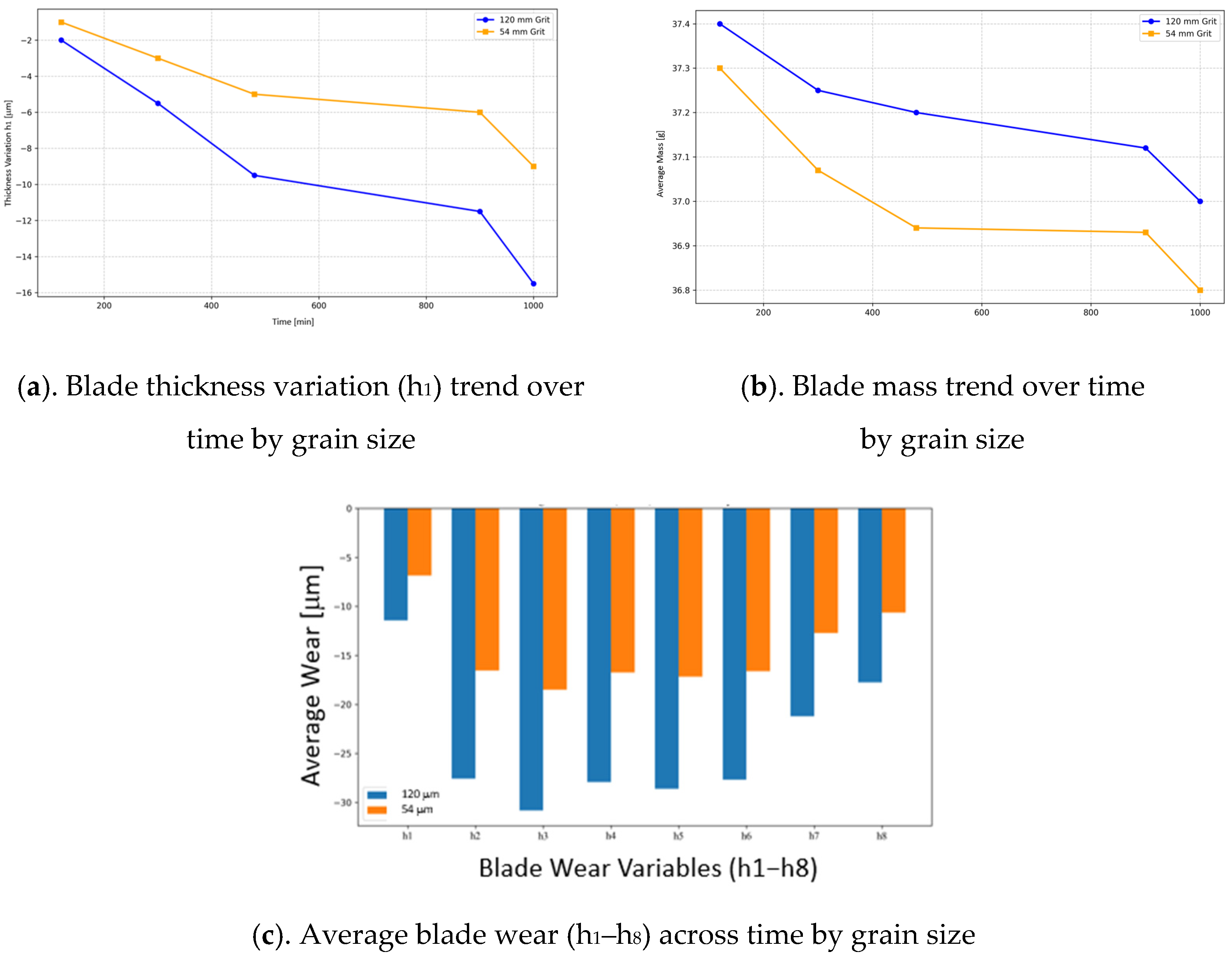
The analysis of grain size effects reveals that the finer 54 µm grit (FEPA F240) mitigates tool wear relative to the coarser 120 µm grit (FEPA F120), as evidenced by h₄ reductions from −28.70 µm to −17.22 µm under equivalent honing conditions, with an absolute decrement of 11.48 µm and statistical validation via t-tests (p < 0.001), thereby endorsing its adoption for prolonged abrasive blade durability and optimized material removal efficiency in sustainable honing workflows. The 120 µm grain size exhibits more significant wear variation and a higher peak wear and mass compared to the 54 µm grain size, which shows more stable wear over time with less extreme fluctuations, as can be seen in Figure 6. Overall, the 120 µm grain size consistently shows higher average wear rates compared to the 54 µm grain size across all variables, with both peaking at h₂ and h₃.

Figure 6. Graphs for analyzing changes caused by grain size.

5. Conclusions

This study presents a robust predictive modeling framework for tool wear (h₁–h₈) and mass loss in honing processes, leveraging machine learning algorithms, support vector regression, random forest, and XGBoost, trained on experimental data from EN-GJL-300 gray cast-iron workpieces using diamond abrasive blades (FEPA F120 and F240). Through 5-fold cross-validation and hyperparameter tuning via GridSearchCV, SVR achieved superior performance for wear predictions (R² = 0.9609–0.9782, MSE = 0.0491–0.0880 µm²), while XGBoost excelled in mass forecasting (R² = 0.9005, MSE = 0.0122 g²). The R² parameter of the SVR model achieves values of approximately 0.97, thus outperforming the ANN in [5] due to the smaller dataset and kernel flexibility. Lower wear, manifested as reduced mass loss, indicates slower material removal from the blade, extending the tool’s lifespan by preserving its structural integrity and functionality. However, if wear is excessively low, the ability to remove material from the workpiece may be compromised, potentially requiring adjustments to process parameters such as pressure or speed. Incorporating grain size as a predictor revealed that finer grains (54 µm) reduced wear by up to 40% compared to coarser ones (120 µm), enhancing prediction reliability and narrowing 95% bootstrap intervals, thus enabling precise process control. The novelty lies in bridging physics-based models with data-driven machine learning, capturing non-linear interactions (quadratic time effects and pressure–speed synergies) via polynomial features (degree 2), addressing gaps in prior roughness-focused studies. These models facilitate adaptive honing optimization, extending tool life, minimizing material waste, and promoting sustainability in automotive and precision engineering under Industry 5.0 paradigms. Future work will prioritize real-time integration through sensor fusion (combining force, vibration, and acoustic emission sensors) with edge machine learning (deploying lightweight models on edge devices for in situ predictions), enabling adaptive control in Industry 5.0 environments to achieve human–machine collaboration for dynamic honing adjustments and enhancing sustainability. To measure the tangential and axial components of the cutting force during honing, piece-holder or honing-holder bar equipment will be developed. In order to measure all the cutting components during honing, it is necessary to record the forces acting at the level of the abrasive blade of the honing tool.

References

- Kalpakjian, S.; Schmid, S.; Vijay Sekar, K.S. Manufacturing Engineering and Technology, 7th ed.; Pearson Education Limited: London, UK, 2021. [Google Scholar]
- Buj-Corral, I.; Sivatte-Adroer, M.; Llanas-Parra, X. Adaptive Indirect Neural Network Model for Roughness in Honing Processes. Tribol. Int. 2020, 141, 105891. [Google Scholar] [CrossRef]
- Rief, S.; Ströer, F.; Kieß, S.; Eifler, M.; Seewig, J. An Approach for the Simulation of Ground and Honed Technical Surfaces for Training Classifiers. Technologies 2017, 5, 66. [Google Scholar] [CrossRef]
- Singh, B.; Bansal, S.; Mishra, P. Artificial Neural Network Modeling and Optimization in Honing Process. Int. J. Comput. Eng. Technol. (IJCET) 2016, 7, 67–77. [Google Scholar]
- Sivatte-Adroer, M.; Llanas-Parra, X.; Buj-Corral, I.; Vivancos-Calvet, J. Indirect Model for Roughness in Rough Honing Processes based on Artificial Neural Networks. Precis. Eng. 2016, 43, 505–513. [Google Scholar] [CrossRef]
- Buj-Corral, S.; Sender, P.; Luis-Pérez, C.J. Modeling of Surface Roughness in Honing Processes by Using Fuzzy Artificial Neural Networks. J. Manuf. Mater. Process. 2023, 7, 23. [Google Scholar] [CrossRef]
- Klein, S.; Schorra, S.; Bähre, D. Quality Prediction of Honed Bores with Machine Learning Based on Machining and Quality Data to Improve the Honing Process Control. In Proceedings of the 53rd CIRP Conference on Manufacturing Systems, Chicago, IL, USA, 1–3 July 2020; pp. 1322–1327. [Google Scholar]
- Deng, Q.; Li, D.; Wang, H.; Cao, P.; Wu, Y. Study of Noise Reduction by Optimizing Ultra-High Speed Milling Parameters by DOE Method. UPB. Sci. Bull. Ser. D 2023, 85, 319–332. [Google Scholar]
- Yang, X.; Li, Y.; Shen, Z.; Chen, R. An Experimental Investigation of Element Diffusion between Cemented Carbide Tools and Titanium Alloys in High Speed Machining Processes. UPB. Sci. Bull. 2020, 82, 225–236. [Google Scholar]
- Gejii, A.; Shukla, S.; Pimparkar, S.; Pattharwala, T.; Bewoor, A. Using a Support Vector Machine for Building a Quality Prediction Model for Center-less Honing Process. Procedia Manuf. 2020, 46, 600–607. [Google Scholar] [CrossRef]
- Qin, F.; Chen, Q.; Tian, X.; Liu, L. Honing Technology based on Intelligent Manufacturing Technology. J. Eng. Mech. Mach. 2022, 7, 12–16. [Google Scholar] [CrossRef]
- Sender, P.; Buj-Corral, I. Influence of Honing Parameters on the Quality of the Machined Parts and Innovations in Honing Processes. Metals 2023, 13, 140. [Google Scholar] [CrossRef]
- Wang, Q.; Chen, X.; An, Q.; Chen, M.; Hun, G.; He, Y. A Tool Wear Prediction and Monitoring Method based on Machining Power Signals. Int. J. Adv. Manuf. Technol. 2023, 129, 5387–5401. [Google Scholar] [CrossRef]
- Chauhan, S.; Trehan, R.; Singh, R.P.; Sharma, V.S. Assessment of Machining Performance for Intelligent Tool Wear Prediction Using Hybrid Extreme Learning Machine. IEEE Sens. J. 2024, 24, 22. [Google Scholar] [CrossRef]
- Mishra, D.; Awasthi, U.; Pattipati, K.R.; Bollas, G.M. Tool Wear Classification in Precision Machining using Distance Metrics and Unsupervised Machine Learning. J. Intell. Manuf. 2025, 36, 331–355. [Google Scholar] [CrossRef]
- Tambake, N.; Deshmukh, B.; Pardeshi, S.; Salunkhe, S.; Cep, R.; Nasr, E. Condition Monitoring of a CNC Hobbing Cutter using Machine Learning Approach. Adv. Mech. Eng. 2024, 16, 16878132241275750. [Google Scholar] [CrossRef]
- Fang, S.; Schorr, S.; Bähre, D. Efficient Machine Learning-Based Forecasting of Key Control Parameters for Analyzing Honing Stone Cutting Performance. In Proceedings of the ASME 20th International Manufacturing Science and Engineering Conference, Greenville, SC, USA, 23–27 June 2025. [Google Scholar]
- Airao, J.; Gupta, A.; Nirala, C.; Wen-Jeng Hsue, A. Bayesian Neural Networks Modeling for Tool Wear Prediction in Milling Al 6061 T6 under MQL Conditions. Int. J. Adv. Manuf. Technol. 2024, 135, 2777–2788. [Google Scholar] [CrossRef]
- Chang, S.H.; Farris, T.N.; Chandrasekar, S. Contact Mechanics of Superfinishing. J. Tribol. ASME 2000, 122, 388–393. [Google Scholar] [CrossRef]
- Heng, L.; Kim, J.S.; Song, J.H.; Mun, S.D. A Review on Surface Finishing Techniques for Difficult-to-Machine Ceramics by Non-Conventional Finishing Processes. Materials 2022, 15, 1227. [Google Scholar] [CrossRef]
- Aslanbaş, İ.G.; Akar, S. Superfinishing Process of Ball Bearings. Çankaya Univ. J. Sci. Eng. 2024, 21, 63–70. [Google Scholar]
- Onishi, T.; Ohashi, K.; Higashi, K.; Morinaka, Y.; Banno, S.; Kitagawa, T.; Tsukamoto, S. In-Process Monitoring of the Machining State in Superfinishing by Measuring the Dynamic Machining Forces. Adv. Mater. Res. 2016, 1136, 592–596. [Google Scholar] [CrossRef]
- Horvath, R.; Dregelyi-Kiss, A.; Matyasi, G. The Examination of Surface Roughness Parameters in the Fine Turning of Hypereutectic Aluminium Alloys. UPB. Sci. Bull. Ser. D 2015, 77, 205–216. [Google Scholar]
- Wang, W.; Shi, S.; Zhang, B.; Jiang, N.; Tang, J. Abrasive Flow Machining Ground Surfaces with Grinding Marks of Different Directions: Parameters Optimization and Mechanisms. J. Manuf. Process. 2025, 148, 212–223. [Google Scholar] [CrossRef]
- Bhowmik, A.; Raja Praveen, K.N.; Bhosle, N.; Gagneja, K. Performance Evaluation of Machine Learning Algorithms in Predicting Machining Responses of Superalloys. AIP Adv. 2024, 14, 105027. [Google Scholar] [CrossRef]
- Lee, S.; Chen, Z.; Luo, Y.; Li, X.; Lu, M. Enhanced Prediction Accuracy in High-speed Grinding of Brittle Materials using Advanced Machine Learning Technique. J. Intell. Manuf. 2024, 36, 5415–5439. [Google Scholar] [CrossRef]
- Kim, G.; Park, S.; Choi, J.; Yang, M.; Lim, S. Developing a Data-Driven System for Grinding Process Parameter Optimization using Machine Learning and Metaheuristic Algorithms. CIRP J. Manuf. Sci. Technol. 2024, 51, 20–35. [Google Scholar] [CrossRef]
- Buj-Corral, I.; Rodero-de-Lamo, L.; Marco-Almagro, L. Optimization and Sensitivity Analysis of the Cutting Conditions in Rough, Semi-Finish and Finish Honing. Materials 2022, 15, 75. [Google Scholar] [CrossRef]
- Fluke 931 Contact and Non-Contact Dual-Purpose Tachometers. Available online: https://www.fluke.com/en-sg/product/building-infrastructure/hvac-tools/fluke-931 (accessed on 23 September 2025).
- National Instruments NI USB-600. Available online: https://www.ni.com/ro-ro/shop/model/usb-6001.html (accessed on 11 September 2025).
- Ohaus Explorer EX124. Available online: https://us.ohaus.com/en-us/products/balances-scales/analytical-balances/explorer-analytical/ex124 (accessed on 22 September 2025).
- Carl Zeiss Universal Microscope. Available online: https://www.zeiss.com/microscopy/en/home.html (accessed on 22 September 2025).
- Ciaburro, G. Regression Analysis with R; Packt Publishing Ltd.: Birmingham, UK, 2018; ISBN 978-1-78862-730-6. [Google Scholar]
- Harrell, F. Regression Modelling Strategies with Applications to Linear Models, Logistic and Ordinal Regression, and Survival Analysis, 2nd ed.; Springer: Berlin/Heidelberg, Germany, 2001. [Google Scholar]
Disclaimer/Publisher’s Note: The statements, opinions and data contained in all publications are solely those of the individual author(s) and contributor(s) and not of MDPI and/or the editor(s). MDPI and/or the editor(s) disclaim responsibility for any injury to people or property resulting from any ideas, methods, instructions or products referred to in the content. |
© 2025 by the author. Licensee MDPI, Basel, Switzerland. This article is an open access article distributed under the terms and conditions of the Creative Commons Attribution (CC BY) license (https://creativecommons.org/licenses/by/4.0/).