Abstract
Sound–colour synaesthesia is a rare phenomenon in which auditory stimuli automatically evoke stable, subjectively real colour experiences. This study aimed to investigate whether the colours most frequently reported by a synesthete can be reliably predicted based on objective acoustic parameters of voice signals. The study analysed the responses of a 24-year-old blind woman to different voices, which she consciously associates with distinct coloured silhouettes. A classification analysis based on MFCC acoustic feature sets and machine learning algorithms (SVM, XGBoost) demonstrated that the models could be trained with very high Accuracy—up to 97–100% in binary classification and 89–90% in multi-class classification. These results provide new insights into how specific sound characteristics are linked to imagery arising from the human subconscious.
1. Introduction
Synaesthesia is an unusual perceptual phenomenon in which individuals experience sensations triggered by the activation of an unrelated sensory modality or cognitive process. These experiences are often accompanied by emotional reactions [1]. Although synaesthesia has been described for centuries, only very recently has scientific research into this condition begun [2]. Synaesthesia is likened to a neurological condition in which a stimulus, called an inducer, which can be sensory (particularly sound or taste) or cognitive (numbers, days, month names), involuntarily, automatically, and consistently evokes a non-externally stimulated sensation, called a concurrent. Synaesthesia is not a conscious decision or choice. It is a passive, unsuppressible experience, although it is triggered by an easily recognisable stimulus [3]. Synaesthesia manifests in various forms: lexical–gustatory synaesthesia (intense taste sensations when looking at letters [4], colour–touch synaesthesia (colour sensations when touching different objects), and spatial–temporal synaesthesia (a spatial experience when thinking about units of time, such as days of the week or months of the year [5,6]. The most common form worldwide is grapheme–colour synaesthesia, in which a person sees letters and corresponding colours arise [7].
It is believed that synaesthesia is inherited in families, which are associated with pronounced structural and functional neuronal differences. It is stated that synesthetic experiences emerge in early childhood and, in adulthood, remain highly automatic and consistent [8,9]. Therefore, it is generally considered a congenital phenomenon [10]. Studies of three or more generations within a single family, using gene ontology analysis, have highlighted six genes—COL4A1, ITGA2, MYO10, ROBO3, SLC9A6, and SLIT2—associated with axonogenesis and expressed in early childhood, when synesthetic associations are formed [11]. However, there are many cases in which synesthetic experiences arise after various brain injuries or head trauma [12]. Synaesthesia following head trauma revealed activation of the left hemisphere during fMRI examination [13]. One reported case involved a 20-year-old woman who, after losing her vision, began to experience visual perception of her hands when she moved them and of the objects she touched. Over the course of a year, these cross-modal sensations developed into vivid visual experiences that accurately reflected her hands, the objects she touched, and, to some extent, objects she could perceive from her immediate surroundings [14]. Although synaesthesia runs in families, its developmental origins are unknown. One prominent hypothesis is that synaesthesia occurs when the hyperconnectivity of cortical connections present in early development does not undergo the normal amount of experience-dependent pruning [15,16]. Another hypothesis about the neural basis of synaesthesia is that individuals exhibit additional neural connectivity and interaction in adjacent cortical areas that process different perceptual features [15,17]. During synaesthesia, altered connectivity in the temporo–occipital and parietal regions may be related to changes in Grey matter. Studies have shown an increased amount of Grey matter in the fusiform and parietal cortex [18]. An increase in white matter volume has also been observed in the bilateral retrosplenial cortex [19,20]. Similarly, other researchers have reported increased cortical thickness, volume, and surface area in the fusiform gyrus and adjacent regions, such as the lingual gyrus and the calcarine cortex, in grapheme–colour synesthetes [20,21]. Synesthetes have been found to have statistically significantly higher serum BDNF levels and thus greater neuroplasticity, compared to a similar control group. Brain-derived neurotrophic factor (BDNF) is one of the most studied neurotrophic factors [22]. In recent years, the measurement of BDNF levels has become a very important area due to its association with various neuropsychiatric disorders [22,23]. Studies of grapheme–colour synaesthesia have shown that when letters and numbers evoke colours, not only are the visual recognition areas of the brain activated, but also the colour-processing area V4 [24]. Synaesthesia is also analysed through the concept of cross-modal perception. The McGurk effect describes the phenomenon in which audition is altered by vision—seeing someone mouth the sound “Faa” while hearing “Baa” makes it impossible to hear anything but “Faa.” Evidence for the interaction of vision with touch and sound has also been shown [25,26,27]. Essentially, there is an ongoing discussion about the structural and functional connectivity of the brain, with two main explanations emerging: (a) cross-activations due to direct connections between functionally or structurally neighbouring cerebral sensory areas [15,22,28] and (b) missing or reduced inhibitory function within the brain, for example, in the form of the disinhibited-feedback model [22,29,30] or the re-entrant-feedback model [6,22].
One problem that has so far hindered research on synaesthesia is the unclear use of the term. For example, cross-sensory metaphors are sometimes described as “synesthetic,” as are additional sensory experiences that arise from the influence of psychedelic drugs, after a stroke, or due to blindness or deafness. Synaesthesia that develops as a result of non-genetic events is called acquired synaesthesia to distinguish it from the more common congenital forms [31]. Synesthetic behaviour can be temporarily induced by cognitive training, verbal suggestion, and drugs [13,32]. Research indicates that synaesthesia can be temporarily experienced by non-synesthetes through the consumption of classic psychedelics such as the partial serotonin receptor agonist lysergic acid diethylamide [32]. However, to determine whether synaesthesia is not artificially induced but rather a permanent, consistent state, the so-called Test of Genuineness (TOG) is used. Some consider the TOG to be the “gold standard” for assessing synaesthesia. In this procedure, synesthetes are asked—either verbally or by matching to a colour palette—to indicate the nature of their synesthetic responses to certain stimuli. They are then retested, often without warning, even after a year or more [33,34]. If a person has synaesthesia, their response consistency in the retesting stage will be significantly higher than that of people without synaesthesia who are simply asked to assign associations to the same set of stimuli [2]. In our previous article, the TOG test had already been carried out for the selected colours [35].
Sound–colour synaesthesia is one of the most common types of synaesthesia. It is thought to occur more frequently in individuals inclined toward creativity and the arts. A heard musical note [36], pitch, tone, or timbre can influence the perception of different colours [37]. EEG studies comparing synesthetes and non-synesthetes have shown significant electrophysiological differences in synesthetes when presented with unimodal auditory stimuli: in synesthetes, an auditory tone is reliably linked to a visual experience, whereas in control groups, it is not [38]. Another study found that two dimensions of musical sound—pitch class and pitch height—were, respectively, associated with the hue–saturation plane and the value/brightness dimension of colour. Mean colour ratings across participants revealed that pitch classes corresponded to rainbow hues, ranging from C—Red; D—Yellow; to B—violet, accompanied by a decrease in saturation. Enharmonic pitch classes, which refer to the same pitch under a different name, evoked colour sensations based on the main pitch class name; for example, C-sharp elicited a Pink sensation, while D-flat was linked to Yellow. Thus, the main factor evoking colour perception was the note name rather than the sound itself [37]. According to an experimental study of synesthetic tendencies involving 104 participants, the “angry” voice in Mozart’s Queen of the Night aria was visualised as Red and Yellow, while a weeping voice was represented by Yellow. “Angelic tones” were perceived as cool colours [39]. In another study, participants strongly associated soft timbres with Blue, green, or light Grey rounded shapes; harsh timbres with Red, Yellow, or dark Grey sharp angular shapes; and mixed timbres (containing both softness and harshness) with a combination of the two shape types. A strong association between the timbre of envelope-normalised sounds and visual shapes was observed [40]. Previous studies have also shown that both the loudness and pitch of auditory stimuli are linked to the brightness and saturation of perceived colours. Pitch, in particular, is associated with colour brightness, whereas loudness is linked to greater visual vividness. Manipulating the spectral content of sounds without changing their pitch revealed that an upward shift in spectral energy was associated with the same visual qualities—greater brightness and saturation—as higher pitch [41]. People reliably associated brighter colours with higher tones and darker colours with lower tones [42]. Sound–colour synaesthesia provides an opportunity to explore the foundations of human perception and the expression of consciousness, offering insight into how sound can be linked to visual colours. Currently, machine learning methods are widely applied in the field of sound analysis. However, in the context of synaesthesia—where the properties of sound are examined through the lens of machine learning—there is very little research available in the literature. Most previous studies have focused on voice signal analysis in other domains, aiming to uncover structural and emotional characteristics of speech. For example, in studies investigating the effect of aging on the human voice, vocal recordings were analysed using the Support Vector Machine (SVM) algorithm. This analysis demonstrated that age-related changes are clearly reflected in the acoustic properties of speech [43]. In other research, machine learning has been used for emotion recognition in speech, evaluating the classification Accuracy for seven or eight emotional categories. Various acoustic features were analysed—such as energy, mel-frequency cepstral coefficients (MFCCs), zero-crossing rate, fundamental frequency, and spectral indicators. The results showed that although subject-independent emotion recognition remains limited, significantly higher Accuracy can be achieved when classifying paired emotions [44]. Moreover, machine learning algorithms have been successfully applied in speech recognition and gender differentiation studies. For instance, Hajin Sarbast [45] applied machine learning in the field of speech recognition, while Wejdan Alsurayyi [46] demonstrated that the Random Forest algorithm, combined with recursive feature elimination (RFE) and 10-fold cross-validation, achieves the highest classification Accuracy in distinguishing male and female voices. J. R. Bock [47] developed and implemented a generative deep neural network to model perception in grapheme–colour synaesthesia. In this model, the weights of the generative network’s hidden layers encode information about pixel intensity, describing the structural features (and identity) of each letter as it is perceived in two dimensions. J. Ward [48], using a machine learning classifier, showed that synesthetes can be distinguished from non-synesthetes using only standard cognitive and personality measures. Importantly, individuals who exhibit multiple forms of synaesthesia display a more distinct profile (i.e., they can be classified with higher Accuracy).
Early computational studies of synaesthesia were largely focused on mappings between sensory modalities, such as associations between colours and musical tones or phonemes, using statistical correlation analyses [49,50]. These approaches provided valuable insights but lacked predictive capability. For example, Asano and Yokosawa [51] demonstrated that Japanese synesthetes most often associate colours with qualitative properties of sound rather than with the visual features of letters; however, this relationship was analysed only statistically, not through a machine learning perspective. Our study proposes a method based on acoustic features extracted from real voice signals (e.g., MFCC coefficients) and applies machine learning algorithms (SVM, XGBoost, RF, LR) to quantitatively predict synesthetic colours with high Accuracy. This approach also reveals a novel way to explore interactions between sensory modalities—specifically, the relationship between sound and colour—from a data-driven perspective by analysing objective signal parameters. Unlike neuroimaging studies [17,18,52], which aim to define the anatomical basis of cross-modal brain connections, our work demonstrates that such connections may be reflected in the structure of acoustic information itself, which can be computationally modeled. This methodological distinction extends machine learning applications beyond neural data analysis toward modelling sensory signal patterns, enabling the study of cross-modality without direct neuroimaging intervention. This approach bridges the fields of synaesthesia, auditory perception, and data science, offering a new way to investigate how sensory associations are interconnected at both biological and computational levels. Our study has two parts. Classification using all colours and four classifiers (Logistic Regression, SVM, RF, and XGBoost) and optimal feature evaluation via sequential feature addition using RF and SVM. The subject of the study was a 24-year-old blind woman who experiences sound–colour synaesthesia. She lost her sight at a young age. Nowadays, after speaking with someone for a certain amount of time, she perceives a coloured silhouette of that person. Therefore, we formulated the hypothesis that specific acoustic properties may be associated with corresponding perceived colours.
2. Materials and Methods
2.1. Study Design
A structured audio-processing method is used to classify spoken audio based on acoustic features (Figure 1). Speech recordings are first digitised and segmented into short- and mid-term frames to extract essential acoustic features, including the following:
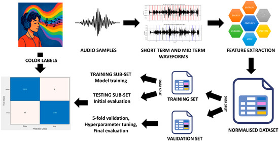
Figure 1.
Audio-processing workflow. The pipeline includes (i) recording, (ii) waveform segmentation, (iii) feature extraction, (iv) normalisation, and (v) stratified data splitting for model training and validation.
- Low-level audio descriptors (LLDs);
- Mel-frequency cepstral coefficients (MFCCs);
- Chroma features (Chroma).
Features are normalised via min–max scaling and organised into a dataset with 136 numerical values and a class label per instance. The dataset consists of around 56,000 samples, which were created using a sliding-window method. It is then split by stratified sampling to ensure the equality of class distribution in both validation and training sets. The training dataset is again split, allowing for both the training of the model and some preliminary testing, while the validation set goes through 5-fold cross-validation and model tuning, serving as the final measure to judge the performance of different models.
2.2. Audio Feature Extraction
Sound was recorded using multi-channel audio equipment at a 44.1 kHz sampling rate. Data preparation for colour classification involved two main stages: (i) extracting features and (ii) selecting the most relevant ones. A total of 18 recorded audio samples were analysed for short-term and mid-term acoustic features (Figure 2).
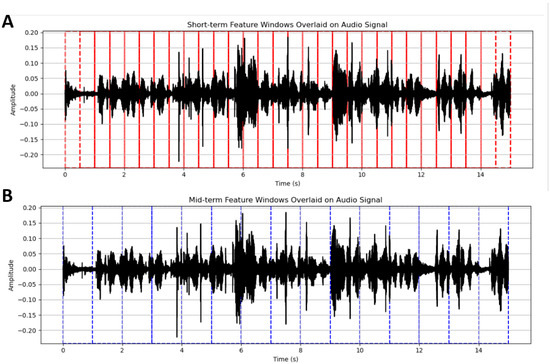
Figure 2.
Visualisation of short-term and mid-term segmentation windows overlaid on an audio waveform. Vertical solid lines indicate the boundaries of the feature analysis windows, dashed lines mark overlap regions between consecutive windows. Colors (red vs. blue) → different time-scale analysis (short-term vs. mid-term). The red lines (A) correspond to short-term windows (~50 ms duration with 25 ms overlap), used to extract frame-level acoustic features. The blue lines (B) represent mid-term windows (~2 s duration with 1 s overlap), which aggregate statistics from the short-term features over longer temporal segments.
For feature extraction, we used the open-source pyAudioAnalysis Python library (https://journals.plos.org/plosone/article?id=10.1371/journal.pone.0144610, The page was opened on 30 June 2025), which offers a variety of audio-signal-processing tools. Short-time feature extraction used overlapping analysis windows so as to grasp the fine-grained temporal and spectral changes within the speech signal. Mid-term features would then be computed as the statistics of the short-term features over longer audio segments. This eliminates temporal redundancy and maintains a stronger representation of audio content over time [53].
A speech recording of approximately five minutes was available, from which between 1514 and 1580 feature vectors were generated. The slight discrepancy in the number of vectors presumably stemmed from differences in the amount of silence interspersed in the recordings that were removed during feature extraction. Thus, the features were extracted from the segmenting and processing of the recordings into two complementary sets of acoustic features: short-term features (ST) and mid-term features (MT). Short-term features were computed using windows of analysis of about 50 ms with an overlap of 25 ms, thereby doing justice to the quick changes in the signal in the temporal and spectral domains.
By analysing small time segments, short-term windows allow for the detection of changes in both timing and frequency of the speech signal. This approach is widely used to extract detailed acoustic features, such as 8 LLDs (low-level audio descriptors), 13 MFCCs (mel-frequency cepstral coefficients), and 13 Chroma (including Chroma std average) features per frame, with their respective standard deviation (standard deviation) values, resulting in 68 short-term features). Mid-term analysis windows provide a statistical summary of short-term features across longer audio segments, allowing for feature representation and reducing redundant temporal information, resulting in another set of 68 features in Appendix A (Table A1).
The LLDs are as follows: zero-crossing rate, energy, entropy, spectral centroid, spectral spread, spectral entropy, spectral flux, and spectral roll-off. The MFCCs represent the shape of the spectral envelope and are generally used to denote the phonetic content of speech. The first few coefficients are most important, as these describe coarse vocal tract resonances and coarse timbral characteristics. Chroma features refer to the 12 semitone pitch class intensities. Such characteristics are helpful in analysing tonal and harmonic structures [54,55].
These features describe spectro-temporal variations. For instance, comparing MFCC profiles from different recordings (e.g., the audio samples associated with “black” and “Pink” colours), we can observe distinct patterns of cepstral traits that encode variations in speaking voice, enunciation, and/or inflection. Such differences are especially pronounced for the first few MFCCs that describe the rough spectral shape of the speech (Figure 3). The first step in this crawling procedure is pre-emphasis, where high-frequency components are emphasised through a high-pass filter. Then, the signal is chopped into small frames with an overlap in-between each frame. Each frame is then multiplied by a window function, such as a Hamming window, to limit spectral leakage, a process known as windowing. Then comes the Fast Fourier Transform (FFT), which converts each frame from the time domain to the frequency domain to provide the power spectrum. The transform is then passed through a bank of Mel Filters, which model the human ear’s level of discrimination by means of a set of triangular filters spaced according to the Mel scale. The output energies are further compressed via a logarithmic function to finish it off with a Discrete Cosine Transform (DCT) that ultimately decorrelates the spectrum and reduces its dimension. The first 12 to 13 coefficients of the resulting Mel-frequency cepstral coefficients (MFCCs) are then taken as a very compact representation of the audio signal. A simplified pipeline is shown in Figure 3.
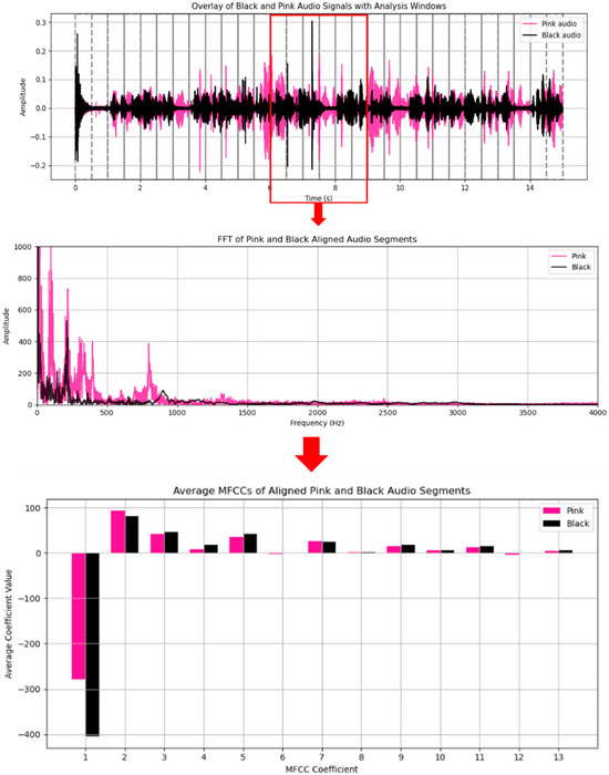
Figure 3.
Spectral and MFCC feature comparison of “Pink”- and “Black”-colour-associated audio segments. The top panel shows the overlay of “Pink” and “Black” audio waveforms with analysis windows, with the red box indicating the segment selected for further analysis. The middle panel presents the Fast Fourier Transform (FFT) spectra of the 3 s aligned segments, highlighting spectral differences around 500 Hz that distinguish the two colour-associated voice samples. The bottom panel shows the average Mel-Frequency Cepstral Coefficients (MFCCs, coefficients 1–13) for the same segments. Distinct patterns between “Pink” and “Black” are visible, especially in MFCCs 2–5 and 7, which relate to timbral and phonetic features.
The output array, structured as [segments × features], was saved as a CSV file. Each row of the file is one audio segment, each column is one of the 136 features that were extracted, and one more “label” column indicates the class of that particular segment (e.g., a colour such as black, Blue, green, etc.). All features were converted into a NumPy array and normalised using min–max scaling, meaning the minimum and maximum are calculated for each feature and then used to scale the rest of the data. A second dataset was created, which includes the standardised features plus the original class labels. This last dataset, saved as CSV, contains around 56 k voice segments of 136 acoustic attributes per record.
2.3. Dataset Partitioning
The dataset includes eight colour classes with varying sample counts: black (10,748), white (9718), Red (9337), Blue (7631), grey (6124), Pink (4721), Yellow (4693), and green (3028). To train and test the models, the data was separated using a 90/10 stratified split. Stratified sampling was applied to deal with the class imbalance and to maintain the proportion of each class in the training and validation sets. This is a way to avoid making model bias [56].
As a result, 90% of the data (approximately 50,400 samples) was used to develop the model, and the remaining 10% (5600 samples) was kept aside as validation. The training set was divided into two subsets, including 40,320 samples for training and 10,080 samples for internal testing. Each sample includes normalised features and a corresponding label indicating its colour class. It is important to know the difference between validation and testing subsets [56]. The training set is used to adequately train the model by adjusting hyperparameters and monitoring its performance during training epochs to prevent overfitting. The validation data, on the other hand, is used to assess the generalisation performance of the final version of the trained model. Intuitively, the assumption should be that a predictor must have greater Accuracy on training data than an unseen one, so if we want to find out how well the model can perform on any new data that appeared in the world, the validation set should never be used. Separation of sets is important to ensure an unbiased evaluation of the likelihood of the model performing well on unseen data [56].
2.4. Non-Binary Multi-Colour Classification
An attempt is made in this section to assess the discriminatory power of acoustic features for classifying eight different colour classes using unsupervised and supervised learning approaches. The classification was performed using a combination of 136 acoustic features coming from two complementary sets of short-term and mid-term features.
Unsupervised classification: Unsupervised k-means clustering has been used in an attempt to characterise the unsupervised separability of the colour classes, given that the prior step was normalisation. The number of clusters to be formed was set equal to the number of unique labels (eight). Metrics of Silhouette Score and Adjusted Rand Index were applied to examine the quality of clustering and to measure the similarity between predicted clusters and actual labels. This would reveal how well the data can naturally be grouped solely by acoustic features.
Supervised Classification: This class of classifications was investigated with a view to choosing the most suitable model for the prediction of colour classes, given acoustic features. The classifiers were chosen for complementary abilities in high-dimensional, multi-class data [57]:
- Logistic Regression (LR);
- Support Vector Machine (SVM);
- Random Forest (RF);
- XGBoost (XGB) [57].
Model training. Each model was trained on a stratified training dataset to ensure balanced class representation. The initial training phase was followed by evaluation on a held-out testing subset, providing a baseline assessment of each model’s generalisation performance. This step allowed us to determine model tendencies (e.g., if the model was overfitting, underfitting or entering minority classes to a degree that performance was degraded) that set the basis for the next hyper-parameter tuning and cross-validation.
Validation. Validation was carried out using the designated validation set, ensuring the models are tested against unseen data to confirm their generalisability, with the 5-fold cross-validation process providing a robust measure of performance consistency across different subsets of the data.
Optimisation. The goal was to maximise the macro-averaged F1-score [58].
Hyperparameter tuning was applied for optimise the performance of each classifier by defining the hyperparameter grids for each model, then using GridSearchCV in 5-fold stratified cross-validation on the validation set to maximise F1-macro score, followed by checking for convergence issues and reporting the best parameters and scores [58].
Afterward, the fine-tuning process gave the following best configuration: RF with 200 trees, maximum depth of 20, without bootstrapping, and default split criteria. For SVM, the best parameters corresponded to the maximum regularisation parameter (C = 10) and gamma being assigned to ‘scale’, which meant that the model had profited from the more involved decision boundary. For LR model the optimal setting was C = 1, penalty = ‘l2’, and solver = ‘saga’. For XGB, the best configuration was 200 estimators, a learning rate of 0.2, maximum depth of 6, and subsampling set to 0.8. The optimal setups were saved for each classifier.
2.5. Binary Classification for Synaesthesia-Related Feature Determination
Feature Grouping: For this purpose, 68 mid-term features were used; the following two-colour groups were evaluated: (i) Blue vs. Pink or (ii) Red vs. Yellow. A complete list of used features is given in Appendix A (Table A1). Features were grouped according to the mean and corresponding standard deviation (std) data: (i) Low-level audio descriptors (LLDs) (features #1–8) and std LLDs (#35–42); (ii) MFCC data—MFCC mean (#9–21) and std MFCCs (#43–55); (iii) Chroma data—Chroma mean (#22–34) and std Chromas (#56–68) (Table A1).
Sequential Feature Selection: Signal samples, corresponding to group I (Blue colour) and group II (Pink colour), were assembled into a single dataset. The initial dataset was split into training and testing sets using an outer 5-fold partition (Figure 4). A single fold, consisting of 1/5 signal patches from group I and group II, was left out as unseen data for the final testing. The remaining 4/5 folds were used for training. Model training was performed simultaneously with feature optimisation, implemented using the “Sequentials” function. The latter determines the optimal feature set following the sequential addition of features. It starts with the feature, leading to the highest classification Accuracy (for the current training/testing data split). If the increment in classification Accuracy is substantial, the new feature is identified as optimal and added to the optimal set of features. The procedure described was repeated five times, resulting in five iterations. A single iteration corresponded to each fold in the outer 5-fold partition. Training/testing split of the initial dataset was performed by setting a random number generator (RNG) to seed #1 (in Matlab R2023b). A similar procedure was performed for Red and Yellow colour differentiation.
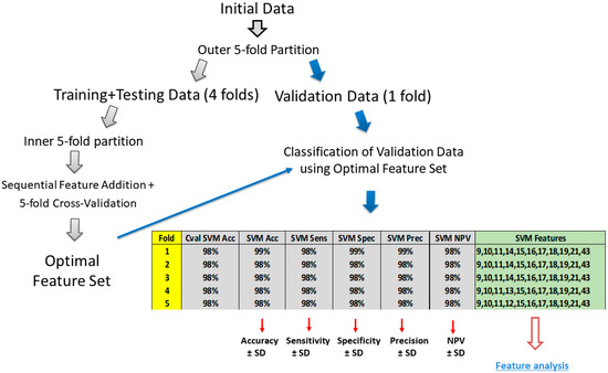
Figure 4.
Binary classification procedure performed simultaneously with optimal feature determination. Initial dataset was split into training/testing and validation datasets using outer 5-fold outer data partition. Single fold was used for final model validation, and remaining four folds were used for model training/testing, coupled with sequential feature optimisation. “SVM” indicates support vector machine classifier. ‘Cval SVM Acc’ indicates Accuracy, obtained during intermediate model testing, on optimal set of features, listed in the column ‘SVM Features’. Other classification metrics were obtained on unseen testing set: Acc—Accuracy; Sens—Sensitivity; Spec—Specificity; Prec—Precision; and NPV—Negative Predictive Value.
A separate, more complex classification, involving a 2-fold data partition, was performed for ½ and ½ data split into training and testing sets.
2.6. Evaluation of Classification Efficiency
For multi-colour classification, we evaluated the model performance via 5-fold cross-validation on the validation set. For every fold, the following per-class metrics were calculated: (i) Accuracy, (ii) Sensitivity (Recall), (iii) Specificity, (iv) Precision, (v) Negative Predictive Value (NPV), and (vi) F1-score. The metrics from each fold were combined to calculate the average (mean) and standard deviation for each class as well as for the overall model.
In binary classification, group I (Blue colour) was marked as 0 (negative) and group II (Pink colour) as 1 (positive). For the classification of Red and Yellow colours, group I (Red colour) was marked as 0 (negative) and group II (Yellow colour) as 1 (positive). Each metric is reported as the mean of all five (outer) folds ± standard deviation of mean. Data analysis was performed using Python 3.11.9, Matlab R2023b (The MathWorks, Inc., Natick, MA, USA), and OriginPro 6.1 (OriginLab Corporation, Microcal, Northampton, MA, USA) software.
3. Results (Part I): Non-Binary Multi-Colour Classification Using All Features
3.1. Clustering
The k-means clustering results showed average performance with an Accuracy of 0.29. This means the unsupervised clustering has difficulty separating the audio features into different colour groups.
The visualisation of k-means clusters (Figure 5A) using Principal Component Analysis (PCA) to reduce dimensions to two components shows a dense, multi-coloured scatter plot, where clusters 0–7 do not align well with true labels, as evidenced by the overlapping points, indicating poor separation and confirming the low Accuracy.
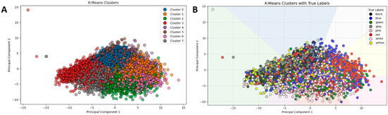
Figure 5.
K-means scatter plots using PCA. Plot (A) displays the clusters (0–7); Plot (B) overlays the same data with true labels.
With its true labels, a second visualisation (Figure 5B) highlights this mismatch, with colours representing actual classes showing significant intermixing, hence accentuating the problem of identifying audio features based on colour associations solely through unsupervised learning.
The figure comprises two scatter plots depicting the results of k-means clustering after the PCA was applied to reduce the dataset to two principal components for ease of interpretation. In Figure 5A, the data points are coloured according to their cluster assignments (labelled 0 through 7), displaying a dense formation with significant overlapping among clusters. The overlap indicates that the clustering algorithm finds it difficult to distinctly separate the samples based on their acoustic properties. Conversely, in Figure 5B, the same data points are plotted but coloured with respect to their actual colour class labels: Black, Blue, Green, Grey, Pink, Red, White, and Yellow. By way of comparison, this clearly reveals a tremendous divergence between the clusters found by the algorithm and the actual class categories, thereby exhibiting the inability of the unsupervised clustering algorithm to effectively model the underlying structure of the data relative to the colour labels. The k-means clustering method recorded Silhouette and ARI values of 0.052 and 0.125, respectively, thereby indicating a weak clustering structure in the feature space.
3.2. Colour Classification
As per the optimisation of the hyperparameters, it was established that both the architecture of the model and parameter settings impacted the classification Accuracy (see Figure 6). Hyperparameter tuning produced the best effects on XGBoost from all processes. With confusion matrices almost perfectly diagonal, along with all other evaluation criteria, XGBoost beats the other models. This can be said to be due to the fact that XGBoost models and also excellently handles intricate, non-linear relations between class imbalance cases and multi-label classification problems. The SVM gained substantially due to tuning, also depending on its ability to deal with complex, non-linear decision boundaries in high dimensions. Random Forest showed a moderate improvement concerning optimised depths and estimators but seemed quite sensitive to the class imbalance. Logistic Regression, despite being a linear model, operated quite reliably and fast, hence endorsing its validity as a baseline.
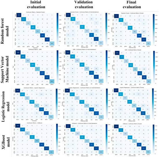
Figure 6.
Logistic Regression (LR), Support Vector Machine (SVM), Random Forest (RF), and XGBoost classifier confusion matrices across three stages of evaluation: The Initial (left column) evaluated on a train–test split without cross-validation or tuning. The Validation (5-fold CV) column (middle) shows average performance values from 5-fold cross-validation on the validation set. The Final (tuned) column (right) depicts the performances of the model after hyperparameter tuning using GridSearchCV and then again evaluated on the validation set. Each matrix visualises classification performance per class (colour label), where the darker the diagonal cell, the stronger the correct prediction consistency.
The range of XGBoost models offers a series of options in terms of Accuracy and generalisation ability, while also endowing the framework with robustness in managing the multi-class synesthetic audio classification task.
3.3. Multi-Colour Classification Metrics for XGBoost and SVM Classifiers
The tuned XGBoost and SVM models exhibited strong and consistent classification performance across the colour classes; as demonstrated in Figure 7, both models received high average values for the main evaluation criteria, Accuracy, Specificity, Precision, Negative Predictive Value (NPV), and F1-score.
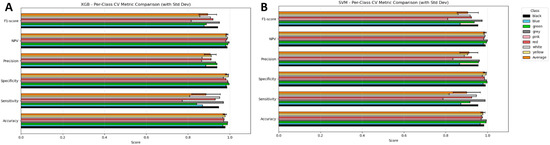
Figure 7.
Per-class cross-validation performance of tuned XGBoost (A) and SVM (B) models across six evaluation metrics: Accuracy, Sensitivity, Specificity, Precision, Negative Predictive Value (NPV), and F1-score. Each coloured bar represents a specific colour class, with the orange bar summarizing the average performance across all classes. Error bars denote standard deviations across folds.
Across all colour classes, XGBoost consistently exhibited the highest performance for F1-score, Specificity, and NPV, where its values typically ranged between 0.95 and 1.0, and where there was little variation observed among the colour classes. Sensitivity displayed more variation than the other parameters, especially for the Red and Pink classes, which yielded lower average scores and larger error margins. This indicates that there were at least occasional inconsistencies with properly identifying true positive cases for these colours. Nonetheless, XGBoost did portray good overall robustness, evidencing excellent Precision and NPV scores, suggesting that the likelihood of XGBoost generating false positives at all was small, and it did very well in accurately identifying negatives.
SVM performed similarly to XGBoost, yielding strong Accuracy and Specificity scores for all classes. Once again, similar to XGBoost, the highest variability was observed among Sensitivity scores, specifically in the Red and Pink classes, also yielding lower average scores. The SVM’s F1-score and Precision scores were also generally more dispersed than those of the XGBoost model, suggesting that its performance, although still highly capable, was slightly less consistent from class to class.
In summary, both models function well, with XGBoost providing marginally more stable and consistent performance than other models. Figure 7 summarises the average (orange bar) across all eight colour classes for each metric, providing a summary of performance metrics that obfuscate class-level variability.
3.4. Average Classification Metrics for All Colours in Multi-Colour Classification
The tables below Table 1 contain the best hyperparameters and macro-F1-score results for tuning the four classifiers. For the SVM, the best parameters to obtain the highest average were an F1-score, gamma = ‘scale’, and kernel = ‘rbf’ (Figure 8), with an average F1-score of 0.8951. Second, the parameter to reach a mean macro F1-score of 0.8875 from XGB were n_estimators = 200, max_depth = 6, learning_rate = 0.2, subsample = 0.8, and colsample_bytree = 1.0. For RF, the maximum hyperparameters were n_estimators = 200, max_depth = 20, and bootstrap was equal to False. The macro-F1-score was 0.8388. For LR, the parameters were C = 1, penalty = ‘l2’, and solver = ‘saga’. The macro-F1-score for LR was 0.8141.

Table 1.
Classification efficiency for 2-fold outer and inner partition using MFFC data, 13 average and 13 standard deviation features.
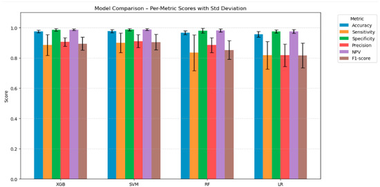
Figure 8.
Bar chart comparing the performance of four tuned classification models across six evaluation metrics. Each bar represents the average metric score across all classes, with error bars showing the standard deviation to reflect performance consistency.
To summarise, SVM offered the best average performance with 98% mean Accuracy, 90% mean Sensitivity, 99% mean Specificity, 91% mean Precision, and 99% mean Negative Predictive Value, with an F1-score of 0.90, suggesting a strong performance with no disadvantage across all evaluation metrics (Figure 8). XGB had, on average, the same performance, just a lower Sensitivity and F1-score. RF had a similar mean performance but also had the same Specificity and Negative Predictive Value. Sensitivity dropped slightly to 0.83, resulting in a decreased F1-score of 0.85. Finally, LR had the worst mean Sensitivity and F1-score (0.82); these scores indicated a decreased ability to correctly identify positive cases. Considering the low variance depicted by the error bars, we could confidently state that the analysis following hyper-parameter tuning could reflect the fit obtained.
These findings suggest that SVM and XGBoost are the most reliable models for this multiclass classification task.
4. Results (Part II): Binary Two-Colour Classification for Feature Analysis
4.1. Classification Efficiency for SVM and RF for Grouped Features
Classification efficiency between two colours, (i) Blue and Pink or (ii) Red and Yellow, was evaluated using an optimal set of features for (i) LLD data (16 features), (ii) MFFC data (26 features), (iii) Chroma data (26 features), and (iv) Overall data (68 features) (Figure 9).
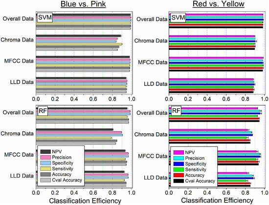
Figure 9.
Classification of (i) Blue and Pink (left panel) or (ii) Red and Yellow (right panel) for SVM and RF classifiers. Cval Accuracy indicates Accuracy obtained during model training; other metrics represent model performance on unseen testing data.
The highest classification efficiency for both binary groups, Blue and Pink or Red and Yellow, was achieved using MFFC and overall data for the SVM classifier, with Accuracy, Sensitivity, Specificity, Precision, and NPV metrics ranging from 95 to 100% classification efficiency (Figure 9). The most efficient group for colour differentiation was the MFFC data for both colour groups.
Compared to SVM, the RF classifier was determined to be less efficient with classification metrics for MFFC data falling into the 90–95% range and, for overall data, increasing to 95% efficiency for both colour groups.
We have obtained high classification efficiency even using a 2-fold outer and inner partition, corresponding to half of the data used for training and half of the data left completely unseen and used for testing of the models (Table 1). The classification using SVM resulted in near-perfect efficiency (95–100%) for all the metrics, with a little lower (90–95%) for the RF classifier.
4.2. Feature Analysis
The analysis of optimal features for the most efficient MFFC data, optimised using 26 features (13 averages and 13 standard deviations), and overall data, using 68 features, is presented for (i) Blue and Pink colours (Figure 10), as well as (ii) for Red and Yellow colours (Figure 11).
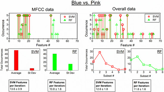
Figure 10.
Features selected into the optimal set for MFFC (left panel) and the overall group (right panel) for the classification of Blue and Pink colours. Summarised occurrences of features within subsets of average and standard deviation data for MFFC features (left middle panel); summarised occurrences for different feature subsets for overall data: 1—LLD average data; 2—MFCC average data; 3—Chroma average data; 4—LDD standard deviation data; 5—MFCC standard deviation data; 6—Chroma standard deviation data (right middle panel). Textboxes indicate the average number of features (±SD) per single iteration. The symbol “#” denotes the feature index number in the feature set list.

Figure 11.
Features selected into the optimal set for MFFC (left panel) and the overall group (right panel) for the classification of Red and Yellow colours. Summarised occurrences of features within subsets of average and standard deviation data for MFFC features (left middle panel); summarised occurrences for different feature subsets for overall data: 1—LLD average data; 2—MFCC average data; 3—Chroma average data; 4—LDD standard deviation data; 5—MFCC standard deviation data; 6—Chroma standard deviation data (right middle panel). Textboxes indicate the average number of features (±SD) per single iteration. The symbol “#” denotes the feature index number in the feature set list.
MFFC data corresponded to the highest classification efficiency between Blue and Pink colours, as it was previously indicated in Figure 9. The dominant optimal features for both SVM and RF classifiers largely corresponded to average features of MFFC data (Figure 10); more than 10 features were required for efficient differentiation.
On the contrary, overall data had all 68 features present in the beginning. Feature distribution has also indicated that average MFFC data was the most dominant for the efficient classification for both SVM and RF classifiers, with approximately 12 features required for the classification.
Similarly, MFFC data corresponded to the highest classification efficiency between Red and Yellow colours (Figure 9). The dominant optimal features for both SVM and RF were average features of MFFC data (Figure 11); more than 11 features were required for efficient differentiation. Classification using overall data has also indicated that average MFFC data was the most dominant for the efficient classification for both SVM and RF classifiers, with approximately 14–15 features required for the classification.
5. Discussion
Sound is one of the most important carriers of information. In a real environment, an audio signal contains a wealth of information about the surroundings. Based on their experience and abilities, people can effectively recognise their environment through sound. The acoustic features used for sound classification must represent the essential characteristics of the audio signal, be reliable, and provide a comprehensive description of it [59]. The main characteristics of the human voice depend on gender, age group, and ethnicity [60]. The use of sound-based machine learning in biomedical research holds considerable promise. In recent years, many researchers have applied acoustic analysis methods [61,62,63,64] to distinguish between two voice quality levels—normal and pathological [61]. Sound-based deep learning methods have shown potential in detecting lung diseases [65]. Recent studies have revealed correlated acoustic features in the voices of patients with depression [66]. Neural networks are widely applied in the study of Parkinson’s disease [67], and in paediatrics, voice feature analysis is used to investigate crying characteristics in infants [68]. In a study of six Japanese synesthetes, it was found that colour choice depended not on the visual appearance of hiragana or katakana characters but on the sounds associated with these characters. The results also demonstrated remarkable consistency [51]. When analysing sounds, loudness and voice quality play a crucial role. Loudness, combined with tense or modal voice quality, can enhance the expression of high-activation states such as formality, indignation, interest, tension, or happiness. Conversely, increasing the loudness of inherently “quiet” voice qualities (breathy, whispered) or decreasing the loudness of inherently “loud” voice qualities (tense) reduces the ability of these qualities to express their associated states [69].
It is believed that the association of vocal qualities with colours in synaesthesia can be expressed at an emotional level. In 1810, Goethe wrote his Theory of Colours, in which he linked categories of colours (e.g., “plus” colours such as Yellow, Red–Yellow, and Yellow–Red) with emotional reactions (e.g., warmth, excitement) [70,71]. Goldstein (1942) expanded on Goethe’s intuition, arguing that certain colours (e.g., Red, Yellow) evoke systematic physiological responses that manifest as emotional experience (e.g., negative arousal), cognitive orientation (e.g., directing attention outward), and overt action (e.g., compelled behaviour). Later theories derived from Goldstein’s ideas focused on wavelength, suggesting that longer-wavelength colours are perceived as exciting or warm, whereas shorter-wavelength colours are perceived as relaxing or cool [71,72]. Colour is considered to have three main attributes: hue, lightness, and chromaticity [73]. Most theories have focused on colour as an independent variable rather than as a dependent one; however, it is also likely that colour perception is influenced by many situational and intrapersonal factors [74]. For example, Jonauskaite et al. [75,76] presented participants with colour-related words and patches and asked them to select the emotions associated with those colours. Their results showed that participants tended to associate anger and love with Red, sadness with Grey, and joy with Yellow, regardless of whether the colours were presented verbally or visually.
Light and dark colours are associated, respectively, with positive and negative emotions: Red with both positive and negative high-arousal emotions; Yellow and orange with positive, high-arousal emotions; Blue, green, Blue–green, and white with positive, low-arousal emotions; Pink with positive emotions; purple with empowering emotions; Grey with negative, low-arousal emotions; and black with negative, high-arousal emotions [77]. Ref. [74] Fetterman presented words related to anger and sadness, written in either Blue or Red, and asked participants to categorise them. Their results showed that anger-related words were categorised more quickly when presented in Red than when presented in Blue, suggesting that the perception of Red—associated with the concept of anger—facilitates the linguistic processing of anger-related content [75].
Although most previous research has focused on subjectively reported associations or neuroimaging data [30,52], systematic attempts to predict these associations using objective acoustic features remain limited. Our study proposes a new approach: by using only acoustic features of voice signals—particularly MFCC—it is possible to reliably classify the most frequently reported synesthetic colour responses. Our results show that, in multi-class classification, SVM and XGBoost models achieved high Accuracy and F1-scores (0.89–0.90). Even in binary classification (e.g., Pink vs. Blue, or Red vs. Yellow), using only 10–15 MFCC features, we achieved more than 97% Accuracy. Although all classification methods (SVM, XGBoost, RF, LR) reached high overall performance, the XGBoost model demonstrated the greatest Accuracy and consistency across all colour classes. This indicates that the foundations of synesthetic perception are not random but are strongly linked to specific phonetic or acoustic structures of speech—possibly because MFCC approximates biological sound perception. This finding supports the hypothesis that synesthetic responses may be driven not only by sensory sound properties but also by emotional perception [78]. It aligns with previous studies reporting consistent links between voice characteristics and colour perception. For example, in [50], higher speech fundamental frequencies and spectral slopes were matched with lighter and pinker colours, “whispering” voices were associated with smoky textures, and “rough” or “creaky” voices were linked to textures resembling dry, cracked soil. Similarly, [49] found that the emotional tone of music (anger, sadness, joy) was associated with specific colours: Red with anger, Yellow with joy, and Blue with sadness. A widely used framework for studying human emotions is James Russell’s [79] circumplex model of affect, which describes emotional responses along two main dimensions: valence (positive to negative) and arousal (low to high) [80]. In this model, emotions are systematically arranged around a circular space, where the X-axis represents valence and the Y-axis represents arousal. Applying Russell’s model to colour perception, colours can be classified by valence and arousal. Pink and Blue fall into the low-to-moderate arousal group. Pink is a warm, emotionally positive colour, often associated with gentleness and softness, while Blue is cool, calming, and linked to relaxation and inner peace. In contrast, Red and Yellow belong to the high-arousal group. Yellow is generally associated with joy, alertness, and high-energy emotions, whereas Red is linked to intense emotional arousal, passion, or even aggression. Both are considered warm colours, but they differ in valence—Yellow tends to be positive, while Red is more ambivalent or negative depending on context—and in perceptual vividness, meaning their visual and emotional impact. These results support the idea that synesthetic colour responses are strongly grounded in both acoustic and emotional aspects of voice, rather than being purely subjective or random sensations. This is in contrast to the previous literature, which has primarily focused on statistical representations of tones and colours. This work predicts colour perception outcomes quantitatively and with high Accuracy by leveraging signal-level acoustic features such as MFCC, LLD, and Chroma. By methodologically integrating the extraction of multivariate acoustic features with machine learning algorithms such as SVM, XGBoost, RF, and LR, a data-driven approach has been provided that can highlight regular correspondences between the voice parameters and perceived colours. It makes a contribution, in that it identifies relationships between acoustic structure and perceived colour, which suggests that cross-modal perceptual mechanisms may be reflected in measurable speech synthesis. Therefore, this study extends the research on synaesthesia beyond descriptive or neuroimaging approaches by introducing a computational method for modelling the individual perceptual representations and providing novel insights into how sound features encode and predict subjective colour experiences.
Limitations and Future Work
This study has shown that machine learning models of colour related to voice activity in blind synaesthesia can be mapped from MFCCs and other acoustic features. We interpret these results that certain acoustic parameters in particular suffice to decompose the reported colour associations by our participant.
Nonetheless, several important limitations need to be noted. The analysis was conducted using data from a single individual whose synaesthetic associations were self-reported and may not reflect the variability observed in the broader synaesthetic population. The high classification Accuracy of the models, while corrected for some bias through stratified sampling and 5-fold cross-validation, suggests that at least some proportion may be capturing within-subject consistency rather than generalisable perceptual patterns. These limitations should be made up for in future works with larger datasets. Additional research is needed with larger numbers of subjects, both within the synesthete population and a control group, but a sample of that kind would be necessary to determine the extent to which patterns, individual differences, and interpersonal Specificity could generalise across synaesthesia types. Moreover, the inclusion of neurophysiological recordings (such as EEG or fMRI) would help make explicit any connections between observed acoustic–colour congruences and neural correlates. Looking at more alternative modelling approaches might instead allow us to model the intrinsic nonlinearities and relations between acoustic features and perceived colour better. It should be assessed whether the synesthetic colour responses corresponded more with acoustic attributes (tone, intensity, timber, or semantic properties of voice type, i.e., emotional content in speech). The present trial is limited in scope; however, its design descriptions lay down a strong methodological framework for broad and more unified multimodal synaesthesia studies between the acoustic, neurophysiological, and machine learning fields.
Author Contributions
R.B.—conceptualisation, software, validation, formal analyses, writing—review and editing. D.R.—software, formal analysis, investigation, writing—original draft preparation, formal analysis. M.M.—software, formal analysis, data curation. G.D.—software, validation. R.R.—software, supervision, project administration. A.S.—formal analysis, supervision, project administration. S.Š.—writing—review and editing, visualisation, supervision, project administration, validation. All authors have read and agreed to the published version of the manuscript.
Funding
This research received no external funding.
Institutional Review Board Statement
The study was conducted in accordance with the Declaration of Helsinki and approved by the Institutional Review Board (or Ethics Committee) of the Faculty of Natural Sciences, Vytautas Magnus University (protocol code 06-09-23, on 6 September 2023 and protocol code 25-04-25, on 25 April 2025).
Informed Consent Statement
Given the simplicity of the procedure, verbal informed consent was obtained from all participants, who voluntarily agreed to take part in the study.
Data Availability Statement
The datasets generated and analyzed during the current study are available from the corresponding author upon reasonable request.
Acknowledgments
The authors would like to thank all study participants. An AI-generated image of a hypothetical synaesthesia perception is given in Figure 1 for illustrative purposes. The image was created using OpenAI’s DALL-E. We also acknowledge the assistance of OpenAI’s ChatGPT (www.chatgpt.com; on 25 September 2025) in refining the English language of this manuscript.
Conflicts of Interest
The authors declare no competing interests.
Appendix A
Table A1.
Feature numbers and groups.
Table A1.
Feature numbers and groups.
| # | Short-Term or Mid-Term Features | LLD Data | MFCC Data | Chroma Data | |
|---|---|---|---|---|---|
| LLD Average | 1 | zcr_mean | + | ||
| 2 | energy_mean | + | |||
| 3 | energy_entropy_mean | + | |||
| 4 | spectral_centroid_mean | + | |||
| 5 | spectral_spread_mean | + | |||
| 6 | spectral_entropy_mean | + | |||
| 7 | spectral_flux_mean | + | |||
| 8 | spectral_rolloff_mean | + | |||
| MFCC Average | 9 | mfcc_1_mean | + | ||
| 10 | mfcc_2_mean | + | |||
| 11 | mfcc_3_mean | + | |||
| 12 | mfcc_4_mean | + | |||
| 13 | mfcc_5_mean | + | |||
| 14 | mfcc_6_mean | + | |||
| 15 | mfcc_7_mean | + | |||
| 16 | mfcc_8_mean | + | |||
| 17 | mfcc_9_mean | + | |||
| 18 | mfcc_10_mean | + | |||
| 19 | mfcc_11_mean | + | |||
| 20 | mfcc_12_mean | + | |||
| 21 | mfcc_13_mean | + | |||
| Chroma Average | 22 | chroma_1_mean | + | ||
| 23 | chroma_2_mean | + | |||
| 24 | chroma_3_mean | + | |||
| 25 | chroma_4_mean | + | |||
| 26 | chroma_5_mean | + | |||
| 27 | chroma_6_mean | + | |||
| 28 | chroma_7_mean | + | |||
| 29 | chroma_8_mean | + | |||
| 30 | chroma_9_mean | + | |||
| 31 | chroma_10_mean | + | |||
| 32 | chroma_11_mean | + | |||
| 33 | chroma_12_mean | + | |||
| 34 | chroma_std_mean | + | |||
| LLD Std Dev | 35 | zcr_std | + | ||
| 36 | energy_std | + | |||
| 37 | energy_entropy_std | + | |||
| 38 | spectral_centroid_std | + | |||
| 39 | spectral_spread_std | + | |||
| 40 | spectral_entropy_std | + | |||
| 41 | spectral_flux_std | + | |||
| 42 | spectral_rolloff_std | + | |||
| MFCC Std Dev | 43 | mfcc_1_std | + | ||
| 44 | mfcc_2_std | + | |||
| 45 | mfcc_3_std | + | |||
| 46 | mfcc_4_std | + | |||
| 47 | mfcc_5_std | + | |||
| 48 | mfcc_6_std | + | |||
| 49 | mfcc_7_std | + | |||
| 50 | mfcc_8_std | + | |||
| 51 | mfcc_9_std | + | |||
| 52 | mfcc_10_std | + | |||
| 53 | mfcc_11_std | + | |||
| 54 | mfcc_12_std | + | |||
| 55 | mfcc_13_std | + | |||
| Chroma Std Dev | 56 | chroma_1_std | + | ||
| 57 | chroma_2_std | + | |||
| 58 | chroma_3_std | + | |||
| 59 | chroma_4_std | + | |||
| 60 | chroma_5_std | + | |||
| 61 | chroma_6_std | + | |||
| 62 | chroma_7_std | + | |||
| 63 | chroma_8_std | + | |||
| 64 | chroma_9_std | + | |||
| 65 | chroma_10_std | + | |||
| 66 | chroma_11_std | + | |||
| 67 | chroma_12_std | + | |||
| 68 | chroma_std_std | + |
References
- Safran, A.; Sanda, N. Color synesthesia. Insight into perception, emotion, and consciousness. Curr. Opin. Neurol. 2015, 28, 36–44. [Google Scholar] [CrossRef]
- Mylopoulos, M.I.; Ro, T. Synesthesia: A colorful word with a touching sound? Front. Psychol. 2013, 4, 763. [Google Scholar] [CrossRef] [PubMed]
- Bragança, G.F.F.; Fonseca, J.G.M.; Caramelli, P. Sinestesia e percepção musical. Dement. Neuropsychol. 2015, 9, 16–23. [Google Scholar] [CrossRef] [PubMed]
- Ward, J.; Simner, J. Lexical-gustatory synaesthesia: Linguistic and conceptual factors. Cognition 2003, 89, 237–261. [Google Scholar] [CrossRef] [PubMed]
- Brang, D.; Rouw, R.; Ramachandran, V.S.; Coulson, S. Similarly shaped letters evoke similar colors in grapheme–color synesthesia. Neuropsychologia 2011, 49, 1355–1358. [Google Scholar] [CrossRef]
- Jarick, M.; Jensen, C.; Dixon, M.J.; Smilek, D. The automaticity of vantage point shifts within a synaesthetes’ spatial calendar. J. Neuropsychol. 2011, 5, 333–352. [Google Scholar] [CrossRef]
- Anash, S.; Boileau, A. Grapheme-Color Synesthesia and Its Connection to Memory. Cureus 2024, 16, e67524. [Google Scholar] [CrossRef]
- Eagleman, D.M.; Kagan, A.D.; Nelson, S.S.; Sagaram, D.; Sarma, A.K. A standardized test battery for the study of synesthesia. J. Neurosci. Methods 2007, 159, 139–145. [Google Scholar] [CrossRef]
- Rothen, N.; Meier, B. Acquiring synaesthesia: Insights from training studies. Front. Hum. Neurosci. 2014, 8, 109. [Google Scholar] [CrossRef]
- Rothen, N.; Meier, B.; Ward, J. Enhanced memory ability: Insights from synaesthesia. Neurosci. Biobehav. Rev. 2012, 36, 1952–1963. [Google Scholar] [CrossRef]
- Tilot, A.K.; Kucera, K.S.; Vino, A.; Asher, J.E.; Baron-Cohen, S.; Fisher, S.E. Rare variants in axonogenesis genes connect three families with sound-color synesthesia. Proc. Natl. Acad. Sci. USA 2018, 115, 3168–3173. [Google Scholar] [CrossRef]
- Abou-Khalil, R.; Acosta, L.M.Y. A case report of acquired synesthesia and heightened creativity in a musician after traumatic brain injury. Neurocase 2023, 29, 18–21. [Google Scholar] [CrossRef]
- Brogaard, B.; Vanni, S.; Silvanto, J. Seeing mathematics: Perceptual experience and brain activity in acquired synesthesia. Neurocase 2013, 19, 566–575. [Google Scholar] [CrossRef] [PubMed]
- Roberts, M.H.; Shenker, J.I. Non-optic vision: Beyond synesthesia? Brain Cogn. 2016, 107, 24–29. [Google Scholar] [CrossRef] [PubMed]
- Hubbard, E.M.; Brang, D.; Ramachandran, V.S. The cross-activation theory at 10. J. Neuropsychol. 2011, 5, 152–177. [Google Scholar] [CrossRef]
- Maurer, D.; Ghloum, J.K.; Gibson, L.C.; Watson, M.R.; Chen, L.M.; Akins, K.; Enns, J.T.; Hensch, T.K.; Werker, J.F. Reduced perceptual narrowing in synesthesia. Proc. Natl. Acad. Sci. USA 2020, 117, 10089–10096. [Google Scholar] [CrossRef] [PubMed]
- Laeng, B.; Flaaten, C.B.; Walle, K.M.; Hochkeppler, A.; Specht, K. ‘Mickey Mousing’ in the Brain: Motion-Sound Synesthesia and the Subcortical Substrate of Audio-Visual Integration. Front. Hum. Neurosci. 2021, 15, 605166. [Google Scholar] [CrossRef]
- Weiss, P.H.; Kalckert, A.; Fink, G.R. Priming Letters by Colors: Evidence for the Bidirectionality of Grapheme–Color Synesthesia. J. Cogn. Neurosci. 2009, 21, 2019–2026. [Google Scholar] [CrossRef]
- Hupé, J.M.; Dojat, M. A critical review of the neuroimaging literature on synesthesia. Front. Hum. Neurosci. 2015, 9, 103. [Google Scholar] [CrossRef]
- Lalwani, P.; Brang, D. Stochastic resonance model of synaesthesia. Philos. Trans. R. Soc. B 2019, 374, 20190029. [Google Scholar] [CrossRef]
- Jäncke, L.; Beeli, G.; Eulig, C.; Hänggi, J. The neuroanatomy of grapheme-color synesthesia. Eur. J. Neurosci. 2009, 29, 1287–1293. [Google Scholar] [CrossRef]
- Eckardt, N.; Sinke, C.; Bleich, S.; Lichtinghagen, R.; Zedler, M. Investigation of the relationship between neuroplasticity and grapheme-color synesthesia. Front. Neurosci. 2024, 18, 1434309. [Google Scholar] [CrossRef]
- Liu, Q.; Balsters, J.H.; Baechinger, M.; Van Der Groen, O.; Wenderoth, N.; Mantini, D. Estimating a neutral reference for electroencephalographic recordings: The importance of using a high-density montage and a realistic head model. J. Neural. Eng. 2015, 12, 56012. [Google Scholar] [CrossRef] [PubMed]
- Sperling, J.M.; Prvulovic, D.; Linden, D.E.J.; Singer, W.; Stirn, A. Neuronal Correlates of Colour-Graphemic Synaesthesia: Afmri Study. Cortex 2006, 42, 295–303. [Google Scholar] [CrossRef] [PubMed]
- Spence, C. Multisensory attention and tactile information-processing. Behav. Brain Res. 2002, 135, 57–64. [Google Scholar] [CrossRef]
- King, A.J.; Calvert, G.A. Multisensory integration: Perceptual grouping by eye and ear. Curr. Biol. 2001, 11, R322–R325. [Google Scholar] [CrossRef] [PubMed]
- Harvey, J.P. Sensory Perception: Lessons from Synesthesia using Synesthesia to inform the understanding of Sensory Perception. Yale J. Biol. Med. 2013, 86, 203–216. [Google Scholar]
- Ramachandran, V.S.; Hubbard, E.M. Synaesthesia—A Window Into Perception, Thought and Language. J. Conscious. Stud. 2001, 8, 33–34. [Google Scholar]
- Grossenbacher, P.G.; Lovelace, C.T. Mechanisms of synesthesia: Cognitive and physiological constraints. Trends Cogn. Sci. 2001, 5, 36–41. [Google Scholar] [CrossRef]
- Neufeld, J.; Sinke, C.; Zedler, M.; Emrich, H.M.; Szycik, G.R. Reduced audio–visual integration in synaesthetes indicated by the double-flash illusion. Brain Res. 2012, 1473, 78–86. [Google Scholar] [CrossRef]
- Hubbard, E.M. Neurophysiology of synesthesia. Curr. Psychiatry Rep. 2007, 9, 193–199. [Google Scholar] [CrossRef]
- Luke, D.P.; Lungu, L.; Friday, R.; Terhune, D.B. The chemical induction of synaesthesia. Hum. Psychopharmacol. 2022, 37, e2832. [Google Scholar] [CrossRef]
- Baron-Cohen, S.; Wyke, M.A.; Binnie, C. Hearing words and seeing colours: An experimental investigation of a case of synaesthesia. Perception 1987, 16, 761–767. [Google Scholar] [CrossRef]
- Asher, J.E.; Aitken, M.R.F.; Farooqi, N.; Kurmani, S.; Baron-Cohen, S. Diagnosing and Phenotyping Visual Synaesthesia: A Preliminary Evaluation of the Revised Test of Genuineness (TOG-R). Cortex 2006, 42, 137–146. [Google Scholar] [CrossRef] [PubMed]
- Bartulienė, R.; Saudargienė, A.; Reinytė, K.; Davidavičius, G.; Davidavičienė, R.; Ašmantas, Š.; Raškinis, G.; Šatkauskas, S. Voice-Evoked Color Prediction Using Deep Neural Networks in Sound–Color Synesthesia. Brain Sci. 2025, 15, 520. [Google Scholar] [CrossRef] [PubMed]
- Rizzo, M.; Eslinger, P.J. Colored hearing synesthesia: An investigation of neural factors. Neurology 1989, 39, 781–784. [Google Scholar] [CrossRef]
- Itoh, K.; Sakata, H.; Kwee, I.L.; Nakada, T. Musical pitch classes have rainbow hues in pitch class-color synesthesia. Sci. Rep. 2017, 7, 17781. [Google Scholar] [CrossRef]
- Goller, A.I.; Otten, L.J.; Ward, J. Seeing Sounds and Hearing Colors: An Event-Related Potential Study of Auditory-Visual Synesthesia. Available online: http://mitprc.silverchair.com/jocn/article-pdf/21/10/1869/1759787/jocn.2009.21134.pdf (accessed on 1 July 2025).
- Takayanagi, K. Colored-hearing synesthesia. Jpn. Hosp. 2008, 27, 51–56. [Google Scholar]
- Adeli, H.; Zhou, Z.; Dadmehr, N. Analysis of EEG records in an epileptic patient using wavelet transform. J. Neurosci. Methods 2003, 123, 69–87. [Google Scholar] [CrossRef]
- Anikin, A.; Johansson, N. Implicit associations between individual properties of color and sound. Atten. Percept. Psychophys. 2019, 81, 764–777. [Google Scholar] [CrossRef]
- Martino, G.; Marks, L.E. Synesthesia: Strong and weak. Curr. Dir. Psychol. Sci. 2001, 10, 61–65. [Google Scholar] [CrossRef]
- Asci, F.; Costantini, G.; Di Leo, P.; Zampogna, A.; Ruoppolo, G.; Berardelli, A.; Saggio, G.; Suppa, A. Machine-learning analysis of voice samples recorded through smartphones: The combined effect of ageing and gender. Sensors 2020, 20, 5022. [Google Scholar] [CrossRef] [PubMed]
- Majkowski, A.; Kołodziej, M. Emotion Recognition from Speech in a Subject-Independent Approach. Appl. Sci. 2025, 15, 6958. [Google Scholar] [CrossRef]
- Sarbast, H. Voice Recognition Based on Machine Learning Classification Algorithms: A Review. Indones. J. Comput. Sci. 2024, 4414–4431. [Google Scholar] [CrossRef]
- Alsurayyi, W.; Aleedy, M.; Alsmariy, R.; Almutairi, S. Gender Recognition by Voice Using Machine Learning. In International Conference on Advanced Network Technologies and Intelligent Computing; Springer International Publishing: Berlin/Heidelberg, Germany, 2024; Volume 6, pp. 7–12. [Google Scholar]
- Bock, J.R. A deep learning model of perception in color-letter synesthesia. Big Data Cogn. Comput. 2018, 2, 8. [Google Scholar] [CrossRef]
- Ward, J.; Filiz, G. Synaesthesia is linked to a distinctive and heritable cognitive profile. Cortex 2020, 126, 134–140. [Google Scholar] [CrossRef]
- Lindborg, P.; Friberg, A.K. Colour Association with Music Is Mediated by Emotion: Evidence from an Experiment Using a CIE Lab Interface and Interviews. PLoS ONE 2015, 10, e0144013. [Google Scholar] [CrossRef] [PubMed]
- Moos, A.; Simmons, D.; Simner, J.; Smith, R. Color and texture associations in voice-induced synesthesia. Front. Psychol. 2013, 4, 568. [Google Scholar] [CrossRef]
- Asano, M.; Yokosawa, K. Synesthetic colors are elicited by sound quality in Japanese synesthetes. Conscious. Cogn. 2011, 20, 1816–1823. [Google Scholar] [CrossRef]
- Hubbard, E.; Ramachandran, V. Neurocognitive Mechanisms of Synesthesia. Neuron 2005, 48, 509–520. [Google Scholar] [CrossRef]
- Giannakopoulos, T. pyAudioAnalysis: An Open-Source Python Library for Audio Signal Analysis. PLoS ONE 2015, 10, e0144610. [Google Scholar] [CrossRef]
- Lukaszewicz, T.; Kania, D. Trajectory of Fifths Based on Chroma Subbands Extraction—A New Approach to Music Representation, Analysis, and Classification. IEEE Trans. Pattern Anal. Mach. Intell. 2025, 47, 2157–2169. [Google Scholar] [CrossRef]
- Abdul, Z.K.; Al-Talabani, A.K. Mel Frequency Cepstral Coefficient and its Applications: A Review. IEEE Access. 2022, 10, 122136–122158. [Google Scholar] [CrossRef]
- Xu, Y.; Goodacre, R. On Splitting Training and Validation Set: A Comparative Study of Cross-Validation, Bootstrap and Systematic Sampling for Estimating the Generalization Performance of Supervised Learning. J. Anal. Test. 2018, 2, 249–262. [Google Scholar] [CrossRef] [PubMed]
- Guo, Y.; Graber, A.; McBurney, R.N.; Balasubramanian, R. Sample size and statistical power considerations in high-dimensionality data settings: A comparative study of classification algorithms. BMC Bioinform. 2010, 11, 447. [Google Scholar] [CrossRef] [PubMed]
- Elgeldawi, E.; Sayed, A.; Galal, A.R.; Zaki, A.M. Hyperparameter Tuning for Machine Learning Algorithms Used for Arabic Sentiment Analysis. Informatics 2021, 8, 79. [Google Scholar] [CrossRef]
- Jin, W.; Wang, X.; Zhan, Y. Environmental Sound Classification Algorithm Based on Region Joint Signal Analysis Feature and Boosting Ensemble Learning. Electronics 2022, 11, 3743. [Google Scholar] [CrossRef]
- Saggio, G.; Costantini, G. Worldwide Healthy Adult Voice Baseline Parameters: A Comprehensive Review. J. Voice 2022, 36, 637–649. [Google Scholar] [CrossRef]
- Rodríguez, P.H.; Ferrer, M.; Travieso, C.; Godino llorente, J.; Díaz-de-María, F. Characterization of Healthy and Pathological Voice Through Measures Based on Nonlinear Dynamics. IEEE Trans. Audio Speech Lang. Process. 2009, 17, 1186–1195. [Google Scholar] [CrossRef]
- Godino-Llorente, J.I.; Gomez-Vilda, P.; Blanco-Velasco, M. Dimensionality Reduction of a Pathological Voice Quality Assessment System Based on Gaussian Mixture Models and Short-Term Cepstral Parameters. IEEE Trans. Biomed. Eng. 2006, 53, 1943–1953. [Google Scholar] [CrossRef]
- Hansen, J.H.L.; Gavidia-Ceballos, L.; Kaiser, J.F. A nonlinear operator-based speech feature analysis method with application to vocal fold pathology assessment. IEEE Trans. Biomed. Eng. 1998, 45, 300–313. [Google Scholar] [CrossRef] [PubMed]
- Eskidere, Ö.; Gürhanli, A. Voice Disorder Classification Based on Multitaper Mel Frequency Cepstral Coefficients Features. Comput. Math. Methods Med. 2015, 2015, 956249. [Google Scholar] [CrossRef]
- Sabry, A.H.; Bashi, O.I.D.; Ali, N.H.N.; Al Kubaisi, Y.M. Lung disease recognition methods using audio-based analysis with machine learning. Heliyon 2024, 10, e26218. [Google Scholar] [CrossRef]
- Ishimaru, M.; Okada, Y.; Uchiyama, R.; Horiguchi, R.; Toyoshima, I. A New Regression Model for Depression Severity Prediction Based on Correlation among Audio Features Using a Graph Convolutional Neural Network. Diagnostics 2023, 13, 727. [Google Scholar] [CrossRef]
- Srinivasan, S.; Ramadass, P.; Mathivanan, S.K.; Selvam, K.P.; Shivahare, B.D.; Shah, M.A. Detection of Parkinson disease using multiclass machine learning approach. Sci. Rep. 2024, 14, 13813. [Google Scholar] [CrossRef]
- Ashwini, K.; Vincent, P.M.D.R.; Srinivasan, K.; Chang, C.Y. Deep Learning Assisted Neonatal Cry Classification via Support Vector Machine Models. Front. Public Health 2021, 9, 670352. [Google Scholar] [CrossRef]
- Yanushevskaya, I.; Gobl, C.; Chasaide, A.N. Voice quality in affect cueing: Does loudness matter? Front. Psychol. 2013, 4, 335. [Google Scholar] [CrossRef]
- Margo, C.E.; Harman, L.E. Helmholtz’s critique of Goethe’s Theory of Color: More than meets the eye. Surv. Ophthalmol. 2019, 64, 241–247. [Google Scholar] [CrossRef] [PubMed]
- Elliot, A.J. Color and psychological functioning: A review of theoretical and empirical work. Front. Psychol. 2015, 6, 127893. [Google Scholar] [CrossRef] [PubMed]
- Goldstein, K. Some Experimental Observations Concerning the Influence of Colors on the Function of the Organism. Occup. Ther. 1942, 21, 147–151. [Google Scholar] [CrossRef]
- Fairchild, M. Color Appearance Models; John Wiley & Sons: Hoboken, NJ, USA, 2013. [Google Scholar]
- Fetterman, A.; Liu, T.; Robinson, M. Extending Color Psychology to the Personality Realm: Interpersonal Hostility Varies by Red Preferences and Perceptual Biases. J. Pers. 2014, 83, 106–116. [Google Scholar] [CrossRef]
- Takei, A.; Imaizumi, S. Effects of color–emotion association on facial expression judgments. Heliyon 2022, 8, e08804. [Google Scholar] [CrossRef]
- Jonauskaite, D.; Abu-Akel, A.; Dael, N.; Oberfeld, D.; Abdel-Khalek, A.M.; Al-Rasheed, A.S.; Antonietti, J.P.; Bogushevskaya, V.; Chamseddine, A.; Chkonia, E.; et al. Universal Patterns in Color-Emotion Associations Are Further Shaped by Linguistic and Geographic Proximity. Psychol. Sci. 2020, 31, 1245–1260. [Google Scholar] [CrossRef]
- Jonauskaite, D.; Mohr, C. Do we feel colours? A systematic review of 128 years of psychological research linking colours and emotions. Psychon. Bull. Rev. 2025, 32, 1457–1486. [Google Scholar] [CrossRef] [PubMed]
- Sithara, A.; Thomas, A.; Mathew, D. Study of MFCC and IHC feature extraction methods with probabilistic acoustic models for speaker biometric applications. Procedia Comput. Sci. 2018, 143, 267–276. [Google Scholar] [CrossRef]
- Russell, J. A Circumplex Model of Affect. J. Pers. Soc. Psychol. 1980, 39, 1161–1178. [Google Scholar] [CrossRef]
- Yin, Y.; Shao, Y.; Hao, Y.; Lu, X. Perceived Soundscape Experiences and Human Emotions in Urban Green Spaces: Application of Russell’s Circumplex Model of Affect. Appl. Sci. 2024, 14, 5828. [Google Scholar] [CrossRef]
Disclaimer/Publisher’s Note: The statements, opinions and data contained in all publications are solely those of the individual author(s) and contributor(s) and not of MDPI and/or the editor(s). MDPI and/or the editor(s) disclaim responsibility for any injury to people or property resulting from any ideas, methods, instructions or products referred to in the content. |
© 2025 by the authors. Licensee MDPI, Basel, Switzerland. This article is an open access article distributed under the terms and conditions of the Creative Commons Attribution (CC BY) license (https://creativecommons.org/licenses/by/4.0/).