The Zero Initial Guess Algorithm for Low-Thrust Trajectory Optimization with Its Application in Cislunar Space

Abstract

In this paper, a trajectory optimization method without an initial value guess is proposed. The method employs the Lagrange multipliers from the nonlinear programming process to estimate the costate of the optimal control problem. It utilizes a homotopic process to address the minimum-fuel problem. The estimated costate serves as a useful initial guess for the indirect shooting method, mitigating the initial value sensitivity. The sequential quadratic programming process used in the shooting process avoids the non-optimal results of the direct method. The minimum-time and minimum-fuel low-thrust rendezvous problems on cislunar L1-vicinity, L2-vicinity, and L2-south near rectilinear halo orbits are solved in this paper. The numerical results demonstrate that using low-thrust propulsion can reduce fuel consumption by 42.36% to 84.62% compared with traditional two-impulse maneuvers in the circular restricted three-body rendezvous problem.

1. Introduction

As humanity ventures into space, cislunar space has garnered significant attention from scholars. The unique orbits within cislunar space are now considered crucial staging grounds for exploring the Moon and embarking on journeys into deep space. China has launched the Queqiao relay satellite, which runs on the halo orbit around the cislunar L2 point [1]. This satellite participates in the exploration plan of the back of the Moon. It maintains the communication chain of the track station and the lunar rover as a relay communication satellite. The Lunar GateWay [2], which is sponsored by the United States, focuses on the 9:2 Southern L2 Near Rectilinear Halo Orbit (NRHO) near the Moon [3]. It aims to construct a space station to support deeper space exploration missions.

To ensure long-term operation and mission expansions, Rendezvous and Docking (RVD) technologies must be developed in special Cislunar orbits. This mission was first proposed in the Apollo program [4], which is considered a linear model of the Circular Restricted Three Body Problem [5,6]. Subsequent research used the relative dynamics model, such as the Elliptic Linear Equations of Relative Motion (ELERM) and Circular Linear Equations of Relative Motion (CLERM) constructed in the Local Vertical Local Horizontal (LVLH) coordinates centered on the Moon [7]. Further developments included the impulse [8] and continuous-thrust maneuver [9] strategies.

In recent years, low-thrust propulsion technologies with higher specific impulse and lower thrust than traditional chemical fuel propulsion have been developed to increase propellant efficiency [10]. As illustrated in Table 1, examples of such technologies include electric propulsion and solar sails, which are suitable for deep space missions. Electric propulsion converts electrical energy into kinetic energy through electrothermal, electrostatic, or electromagnetic means. Solar sails, conversely, use a lightweight, highly reflective membrane to reflect photons and generate thrust from solar radiation pressure. For the rendezvous problem, electric propulsion is more suitable for closer missions, whereas solar sail has not yet been successfully applied owing to its lower thrust and the more complex sail controls involved (including control of the sail and support mechanisms). These new methods lead to low-thrust control strategies, such as the Linear Quadratic Regulator (LQR) [11] controller.

Table 1. Typical propulsion technologies and their performance.

Propulsion Mode	Technology	Thrust Range	Specific Impulse	Mission/Project
	Cold gas	10 $\mathsf{\mu }$N–3.6 N	40–110 s	CanX-4 [12]
Chemical fuel	Hydrazine	0.25–28 N	180–285 s	CAPSTONE [13]
	Biopropellants	50 mN–22 N	150–310 s	Cislunar Explorers [14]
	Hall-Effect	0.25–55 mN	200–1920 s	SMART-1 [15]
Electric	Gridded Ion	0.1–20 mN	500–2400 s	GOCE [16]
	Electrosprays	20 $\mathsf{\mu }$N–350 mN	225–3000 s	ICEYE-X2 [17]
Propellantless	Solar sail	$\mathsf{\mu }$N∼mN	-	ACS3 [18]

Compared to conventional optimization methods based on impulse maneuvers, the low-thrust propulsion mode introduces a higher dimensionality to the optimization problem, thereby increasing its complexity. This low-thrust trajectory optimization problem is typically solved by the direct method [19] or indirect method [20]. The optimization variable for the indirect method is the initial costate, which usually requires a good initial guess to ensure convergence. The direct method directly optimizes the control law without considering the necessary conditions; hence, the solution set is usually suboptimal. Although some techniques have been proposed to reduce the influence of the initial costate, such as the homotopic method [21,22] and the continuation method [23,24], most researchers prefer a hybrid approach that incorporates the heuristic algorithm [25]. However, a significant issue with these methods is their lack of robustness, as they can produce different results from the same initial state. While traditional impulsive propulsion has been applied in the Apollo program [4], low-thrust propulsion technologies (e.g., electric propulsion, solar sails) with higher specific impulse (Table 1) are preferred for deep-space missions. However, low-thrust trajectory optimization has higher dimensionalit. This highlights the need for an efficient algorithm without initial guesses.

In this manuscript, we propose a Zero Initial Guess Algorithm (ZIGA) for trajectory optimization to solve the low-thrust rendezvous problem in cislunar space. For the most challenging Minimum-Fuel (MF) problem in low-thrust trajectory optimization, ZIGA employs a two-stage relay solution approach. Taheri et al. [20] proposed a costate mapping method, but it relies on high-quality initial NLP solutions. Zhang et al. [22] developed a homotopic method, but it lacks an intermediate auxiliary problem to stabilize iteration. ZIGA addresses these limitations by using the ME problem to link NLP-based costate mapping and the homotopic process, filling the gap in existing methods. The first stage solves an auxiliary problem similar to the minimum-fuel problem—the Minimum-Energy (ME) problem. In the second stage, the initial costate for the ME problem is first obtained through costate mapping. Subsequently, iterative optimization is performed by gradually adjusting the cost function, which leads to the derivation of the initial costate for the MF problem. Finally, a direct forward integration yields the optimal fuel rendezvous trajectory and optimal control law. Specifically, in the first stage, ZIGA uses the Radau pseudospectral method (RPM) to formulate a nonlinear programming (NLP) problem and solve it to obtain the optimal control law for the ME problem. Because RPM satisfies the costate mapping principle (from our previous work [26]), we utilize the process variables from the first stage (the Lagrange multipliers of the NLP) in the second stage to map the initial costate for the ME problem. Subsequently, a sequence of homotopic parameters with progressively decreasing step sizes is constructed, and the MF problem is iteratively solved using the SQP algorithm. This method does not require any initial guesses regarding state variables, control laws, or costates and considers Pontryagin’s minimum principle during the homotopic process to obtain the optimal solution. In addition, for minimum-time problems that are less sensitive to initial values, only the first stage of ZIGA is required to obtain the optimal solution.

The remainder of this paper is structured as follows. Section 2 presents the spacecraft dynamics equations and methods for calculating periodic orbits. Section 3 establishes the low-thrust rendezvous problem and derives the analytical optimal control law. Section 4 provides a detailed introduction to ZIGA. Section 5 performs numerical simulations, compares them with existing algorithms, and analyzes the performance of ZIGA. Section 6 presents conclusions and possible future works.

2. Spacecraft Dynamics and Halo Orbit

2.1. Circular Restricted Three-Body Problem

Typically, the motion of the spacecraft in cislunar space is approximated as a Circular Restricted Three Body Problem (CR3BP) [27]. In this model, the Earth and the Moon move in a circular plane around the common center of mass. The motion of the spacecraft is influenced by the combined gravitational force of both, and the mass is ignored.

In the Earth–Moon CR3BP, the Earth–Moon rotating frame is deemed useful. As illustrated in Figure 1, this frame exhibits the x-axis along the Earth–Moon position vector, the z-axis along the angular momentum vector of the Moon’s orbit, and the y-axis completes the orthogonal system, with the center located at the barycenter. Considering the control of low-thrust vector $\mathit{u}$, the dynamic equation is written as

$$\begin{array}{c}\hfill \dot{\mathit{X}}=\mathit{f}(\mathit{X},\mathit{u})=\left[\begin{array}{c}\dot{\mathit{r}}\\ \dot{\mathit{v}}\\ \dot{m}\end{array}\right]=\left[\begin{array}{c}\mathit{v}\\ \mathit{g}\left(\mathit{r}\right)+\mathit{h}\left(\mathit{v}\right)+{\displaystyle \frac{\mathit{u}{T}_{\max }}{m}}\\ {\displaystyle \frac{-u{T}_{\max }}{I_{\mathrm{sp}}{g}_0}}\end{array}\right]\end{array}$$

(1)

where $\mathit{r}=[r_x,r_y,r_z]$ and $\mathit{v}=[v_x,v_y,v_z]$ are the position and velocity of the chaser and the target spacecraft, respectively. m denotes the mass of the spacecraft. $u=\left|\mathit{u}\right|$ represents the norm of the control $\mathit{u}$. $T_{\max }$ is the maximum allowable thrust. $I_{\mathrm{sp}}$ is the propellant specific impulse, and $g_0$ is the gravitational acceleration at the sea level.

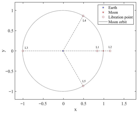
Figure 1. Planets and libration points in the Earth–Moon rotating frame.

The $\mathit{g}\left(\mathit{r}\right)$ and $\mathit{h}\left(\mathit{v}\right)$ are defined as

$$\begin{array}{ccc}\hfill \mathit{g}\left(\mathit{r}\right)& =& \left[\begin{array}{c}{r}_x-{\displaystyle \frac{(1-\mu )(r_x+\mu )}{r_1^3}}-\mu {\displaystyle \frac{r_x+\mu -1}{r_2^3}}\\ r_y-{\displaystyle \frac{(1-\mu )r_y}{r_1^3}}-\mu {\displaystyle \frac{r_y}{r_2^3}}\\ -{\displaystyle \frac{(1-\mu )z}{r_1^3}}-\mu {\displaystyle \frac{r_z}{r_2^3}}\end{array}\right]\hfill \end{array}$$

(2)

$$\begin{array}{ccc}\hfill \mathit{h}\left(\mathit{v}\right)& =& \left[\begin{array}{c}2v_y\\ -2v_x\\ 0\end{array}\right]\hfill \end{array}$$

(3)

where $r_1={[{(r_x+\mu )}^2+r_y^2+r_z^2]}^{1/2}$ and $r_2={[{(r_x+\mu -1)}^2+r_y^2+r_z^2]}^{1/2}$ represent the distance between the spacecraft and the primary and secondary planet, respectively. $\mu =0.01215$ is the normalized value of the mass of the moon.

2.2. Construction of Cislunar Halo Orbit

2.2.1. Richardson Analytical Solution

Richardson proposed an analytical solution of the halo orbit in the CR3BP [28]. The complete third-order form is

$$\begin{array}{c}\hfill \begin{array}{cc}\hfill \tilde{x}=& a_{21}{A}_x^2+a_{22}{A}_z^2-A_x\cos \left({\tau }_1\right)+(a_{23}{A}_x^2-a_{24}{A}_z^2)\cos \left(2{\tau }_1\right)\hfill \\ & +(a_{31}{A}_x^3-a_{32}{A}_x{A}_z^2)\cos \left(3{\tau }_1\right)\hfill \\ \hfill \tilde{y}=& k{A}_x\sin \left({\tau }_1\right)+(b_{21}{A}_x^2-b_{22}{A}_z^2)\sin \left(2{\tau }_1\right)+(b_{31}{A}_x^3-b_{32}{A}_x{A}_z^2)\sin \left(3{\tau }_1\right)\hfill \\ \hfill \tilde{z}=& {\delta }_n{A}_z\cos \left({\tau }_1\right)+{\delta }_n{d}_{21}{A}_x{A}_z(\cos \left(2{\tau }_1\right)-3)+{\delta }_n(d_{32}{A}_z{A}_x^2-d_{31}{A}_z^3)\cos \left(3{\tau }_1\right)\hfill \end{array}\end{array}$$

(4)

where $A_x$ and $A_z$ denote the amplitudes on x- and z-axes, respectively. ${\tau }_1$ represents the phase of the orbit. The definitions of the remaining coefficients ($a_{21}$ $a_{22}$ $a_{23}$ $a_{24}$ $a_{31}$ $a_{32}$ $b_{21}$ $b_{22}$ $b_{31}$ $b_{32}$ $d_{21}$ $d_{31}$ $d_{32}$ k ${\delta }_n$) can be found in the original article.

By finding the derivative of Equation (4), We can obtain the analytical form of the velocity

$$\begin{array}{c}\hfill \begin{array}{cc}\hfill \dot{\tilde{x}}& =A_x\sin \left({\tau }_1\right)-2(a_{23}{A}_x^2-a_{24}{A}_z^2)\sin \left(2{\tau }_1\right)-3(a_{31}{A}_x^3-a_{32}{A}_x{A}_z^2)\sin \left(3{\tau }_1\right)\hfill \\ \hfill \dot{\tilde{y}}& =k{A}_x\cos \left({\tau }_1\right)+2(b_{21}{A}_x^2-b_{22}{A}_z^2)\cos \left(2{\tau }_1\right)+3(b_{31}{A}_x^3-b_{32}{A}_x{A}_z^2)\cos \left(3{\tau }_1\right)\hfill \\ \hfill \dot{\tilde{z}}& =-{\delta }_n{A}_z\sin \left({\tau }_1\right)-2{\delta }_n{d}_{21}{A}_x{A}_z\sin \left(2{\tau }_1\right)-3{\delta }_n(d_{32}{A}_z{A}_x^2-d_{31}{A}_z^3)\sin \left(3{\tau }_1\right)\hfill \end{array}\end{array}$$

(5)

2.2.2. Direct Shooting Method Based on State-Transition-Matrices

The analytical solution provides an initial guess for the target’s numerical halo orbit $[x,y,z,\dot{x},\dot{y},\dot{z}]$. In recent research, scholars utilized a numerical approach to obtain the exact halo orbit [29], which is called the Direct Shooting Method (DSM). From the basic differential correct theory, we assume that $\delta z=0$; thus, the correction of the state can be calculated by

$$\begin{array}{c}\hfill \left[\begin{array}{c}\delta x\\ \delta \dot{y}\\ \delta t\end{array}\right]={\left[\begin{array}{ccc}{\Phi }_{21}& {\Phi }_{25}& \dot{y}\\ {\Phi }_{41}& {\Phi }_{45}& \ddot{x}\\ {\Phi }_{61}& {\Phi }_{65}& \ddot{z}\end{array}\right]}^{-1}\left[\begin{array}{c}0\\ \delta \dot{x}\\ \delta \dot{z}\end{array}\right]\end{array}$$

(6)

where $\Phi$ represents the state transition matrix of the dynamics in Equation (1); the subscripts denote its elements.

3. Low-Thrust Rendezvous Problem

3.1. Minimum-Time Problem

The minimum-time (MT) problem implies that the objective function is $J={\int }_{t_0}^{t_f}dt$, and the control of the chaser is $\mathit{u}=-{\displaystyle \frac{T_{\max }{\mathit{\lambda }}_v}{{\lambda }_v}}$. We can obtain the Hamilton function as follows:

$$\begin{array}{c}\hfill H={\mathit{\lambda }}_r\mathit{v}+{\mathit{\lambda }}_v\left[\mathit{g}\left(\mathit{r}\right)+\mathit{h}\left(\mathit{v}\right)+{\displaystyle \frac{\mathit{u}{T}_{\max }}{m}}\right]-{\lambda }_m{\displaystyle \frac{u{T}_{\max }}{I_{\mathrm{sp}}{g}_0}}+1\end{array}$$

(7)

where $\mathit{\lambda }=[{\mathit{\lambda }}_{\mathit{r}},{\mathit{\lambda }}_{\mathit{v}},{\lambda }_m]$ denotes the costate vector. Since the final time is free, the optimize parameter is $[\mathit{\lambda },t_f]$ and has 8 dimensions. Furthermore, the unconstrained final mass results in an associated costate at the final time of ${\lambda }_m\left(t_f\right)=0$ [30]. Combined with the rendezvous requirements and the transversality condition $H\left(t_f\right)=0$ [31] associated with the final free time, the 8-dimensional constraints are given by

$$\begin{array}{c}\hfill \mathit{\varphi }({[\mathit{X},\mathit{\lambda }]}^{\mathrm{T}},t_0,t_f)=\left[\begin{array}{c}\mathit{r}\left(t_f\right)-{\mathit{r}}_f\\ \mathit{v}\left(t_f\right)-{\mathit{v}}_f\\ {\lambda }_m\left(t_f\right)\\ H\left(t_f\right)\end{array}\right]={\mathbf{0}}_8\end{array}$$

(8)

where ${\mathit{r}}_f=[x,y,z]$ and ${\mathit{v}}_f=[\dot{x},\dot{y},\dot{z}]$ represent the target’s halo orbit.

3.2. Minimum-Fuel Problem

The minimum-fuel (MF) problem signifies that the objective function is $J={\int }_{t_0}^{t_f}udt$, and the control of the chaser is $\mathit{u}=-{\displaystyle \frac{u{\mathit{\lambda }}_v}{{\lambda }_v}}$ with $u\in [0,T_{\max }]$. Therefore, the Hamilton function is

$$\begin{array}{c}\hfill \begin{array}{cc}\hfill H=& {\mathit{\lambda }}_r\mathit{v}+{\mathit{\lambda }}_v\left[\mathit{g}\left(\mathit{r}\right)+\mathit{h}\left(\mathit{v}\right)+{\displaystyle \frac{\mathit{u}{T}_{\max }}{m}}\right]-{\lambda }_m{\displaystyle \frac{u{T}_{\max }}{I_{\mathrm{sp}}{g}_0}}\hfill \\ & +{\displaystyle \frac{T_{\max }}{I_{\mathrm{sp}}{g}_0}}\left[u-ϵu(1-u)\right]\hfill \end{array}\end{array}$$

(9)

In this equation, $ϵ$ gradually decreases in a homotopic process from minimum-energy (ME) problem ($ϵ=1$) to minimum-fuel problem ($ϵ=0$). After applying the Protrygin minimum principle, the switching function is

$$\begin{array}{c}\hfill S=-{\mathit{\lambda }}_v{\displaystyle \frac{I_{\mathrm{sp}}{g}_0}{m}}-{\mathit{\lambda }}_m+1\end{array}$$

(10)

In the minimum-fuel problem, the final time is fixed, and the optimization parameter is $\mathit{\lambda }$ with 7 dimensions. As described in Section 3.1, applying the boundary condition for the final costate of mass results in the complete 7-dimensional terminal constraint as

$$\begin{array}{c}\hfill \mathit{\varphi }({[\mathit{X},\mathit{\lambda }]}^{\mathrm{T}},t_0,t_f)=\left[\begin{array}{c}\mathit{r}\left(t_f\right)-{\mathit{r}}_f\\ \mathit{v}\left(t_f\right)-{\mathit{v}}_f\\ {\lambda }_m\left(t_f\right)\end{array}\right]={\mathbf{0}}_7\end{array}$$

(11)

4. Zero Initial Guess Algorithm for Trajectory Optimization

4.1. Costate Mapping Process

The traditional direct method discretizes the state and control at specific collocation points, thereby transforming the original optimal control problem into a Nonlinear Programming (NLP) problem [26]. Meanwhile, the indirect method utilizes the necessary condition to transform the original problem into a Two-Point Boundary Value Problem (TPBVP). In the NLP, the parameters to be optimized are discrete states and controls, whereas in TPBVP, they are the initial costates and the rendezvous time (optional).

Gaussian quadrature rules, Lagrange multipliers, and differential matrices serve as intermediate processes/parameters in the NLP process for estimating discrete states and controls. Furthermore, the Karush–Kuhn–Tucker condition for NLP is consistent with the discrete form of the first-order necessary condition, which includes the costate. This relationship is known as costate mapping [32] and connects the Gaussian orthogonal quadrature weights, Lagrange multipliers, and differential matrices with discrete costate:

$$\begin{array}{c}{\tilde{\mathit{\lambda }}}_k={\displaystyle \frac{{\mathbf{\Lambda }}_k}{{\omega }_k}},(k=1,\dots ,N)\end{array}$$

(12)

$$\begin{array}{c}{\tilde{\mathit{\lambda }}}_{N+1}={\mathbf{D}}_{N+1}^{\mathrm{T}}\mathbf{\Lambda }\end{array}$$

(13)

where ${\mathbf{\Lambda }}_k$ denotes the kth row of the Lagrange multiplier matrix $\mathbf{\Lambda }$ and ${\mathbf{D}}_{N+1}^{\mathrm{T}}$ is the $(N+1)$th column of the differential matrix $\mathbf{D}$. ${\omega }_k$ is the orthogonal weight [33].

The direct method does not always provide an optimal estimation of the costate, particularly in cases where the solution is non-smooth [19]. In such instances, the discrete costate may diverge from the optimal costate. Consequently, we propose utilizing the discrete costate as the initial guess for the TPBVP. We obtain the optimal solution for the initial costate and final time by solving local optimization problems. This two-stage solution framework greatly reduces the sensitivity problem of indirect methods and overcomes convergence issues. In Stage 1 of the ZIGA, the hp-adaptive Radau pseudospectral method (RPM) was used to obtain the estimated rendezvous time.

The mapped costate ${\lambda }_v$ (velocity-related costate) directly correlates with the thrust direction; the vector direction of ${\lambda }_v$ is opposite to the optimal thrust direction, and its magnitude reflects the priority of thrust adjustment. A larger $\parallel {\lambda }_v\parallel$ indicates a higher need to adjust thrust to correct velocity deviations. The costate ${\lambda }_m$ (mass-related costate) is linked to fuel consumption rate; a decrease in ${\lambda }_m$ means the algorithm prioritizes reducing thrust output to save fuel. For halo orbits (e.g., L2-vicinity orbits with complex gravitational fields), ZIGA uses costate mapping to adaptively adjust thrust; in unstable orbital regions (e.g., near the L2 libration point), ${\lambda }_m$ decreases to avoid excessive fuel consumption, ensuring trajectory stability and fuel efficiency.

4.2. Homotopic Process

In Stage 2, first, the costate mapping process is utilized to obtain the discrete costate. Then, Sequential Quadratic Programming (SQP) is used to find the optimal costate. Next, we begin the homotopic process using the result of the costate mapping as the first generation. The relationship between the ZIGA and three typical optimization problems is illustrated in Figure 2.

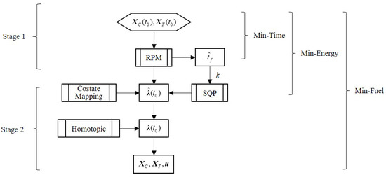
Figure 2. The Zero Initial Guess Algorithm for trajectory optimization.

The Minimum-time problem can be solved using only Stage 1, whereas the Min-fuel problem requires both stages of the ZIGA. To solve the Min-fuel problem, the costate of the ME problem is given by the costate mapping process. Because the RPM is a direct collocation method with a non-optimal solution, we need to find the optimal costate at $ϵ=1$ before the homotopic process. Subsequently, we use a sequence gradually decreasing the homotopic coefficient $ϵ$ as

$$\begin{array}{c}\hfill ϵ={\displaystyle \frac{i^2-1}{99}}\end{array}$$

(14)

where $i=10,9,\dots ,1$ represents the 10 iteration steps corresponding to $ϵ=1$ to $ϵ=0$. In each iteration, an indirect shooting process is constructed and solved by the SQP.

4.3. Novelty and Contribution

Methodological Integration Innovation: Unlike the single costate mapping method by Taheri & Junkins [20] which relies on high-quality initial NLP solutions, and the homotopic process by Zhang et al. [22] which lacks an intermediate auxiliary problem, ZIGA uniquely couples the hp-adaptive Radau Pseudospectral Method (RPM)-based NLP costate mapping with a sequential homotopic process. The Minimum-Energy (ME) problem acts as a bridge to connect these two stages, eliminating the initial guess sensitivity of indirect methods and the divergence risk of standalone homotopic methods.

Mathematical Formulation Innovation: We propose a decreasing homotopic coefficient sequence defined by Equation (14), which enables a smooth transition of $ϵ$ from 1 (ME problem) to 0 (Minimum-Fuel (MF) problem). This avoids abrupt changes in the control law and ensures stable iteration, a key improvement over arbitrary coefficient sequences in existing studies.

5. Numerical Results

5.1. ZIGA to the Low-Thrust Rendezvous Problem

This section utilizes the Zero Initial Guess Algorithm to solve three typical low-thrust rendezvous problems and compares them to the results of traditional impulsive maneuvers, known as the Three-Body Lambert Problem (TBLP). The initial orbits of the target and chaser are chosen from three typical cislunar halo orbits.

5.1.1. L1-Vicinity Halo Orbit

Halo orbits around L1 are typically chosen for scientific missions [34]. In the rendezvous scenario, an L1 southern halo orbit with an amplitude of 5000 km in the z-axis and a period of 11.99 days is used for the target and chaser spacecraft. We assume that the Chaser is at 0 degrees ($r_y=0$) at the start time, whereas the Target is at 12.5 degrees. In the ME and MF problems, we assume that the rendezvous time is 0.25 halo orbital periods. In Stage 1 of ZIGA, the tolerance ${10}^{-5}$ is used for a fast solution of the MT and ME problem, and in Stage 2, ${10}^{-15}$ is used for high accuracy. Additionally, $T_{\max }$ = 30 mN, $I_{\mathrm{sp}}$ = 3000 s and m = 1500 kg is used for the Chaser.

In Figure 3, Figure 4 and Figure 5, I denotes initial position, F denotes final position, O denotes rendezvous orbit, subscript C denotes chaser, and T denotes target. Words in brackets represent the rendezvous problem. The final positions of the ME problem, MF problem, and TBLP coincide owing to the fixed final time. However, the result of the MT problem leads to a phase ahead of them in the halo orbit, representing less time consumption for rendezvous.

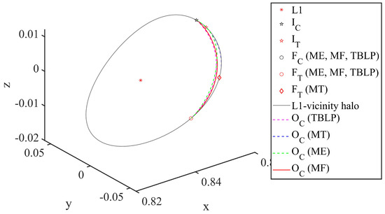
Figure 3. Rendezvous trajectories on the L1-vicinity halo orbit in the Earth–Moon rotating frame.

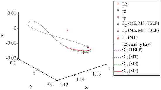
Figure 4. Rendezvous trajectories on the L2-vicinity halo orbit in the Earth–Moon rotating frame.

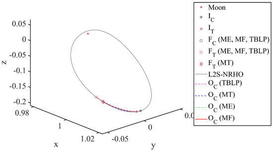
Figure 5. Rendezvous trajectories on the L2-South near Rectilinear Halo Orbit in the Earth–Moon rotating frame.

To resolve the rendezvous problem on halo orbit, typically, appropriate values for $\mathit{\lambda }\left(t_0\right)$ and $t_f$ must be selected. In the MT problem, it is known that the engine will invariably utilize the maximum available thrust [35]. Including this prior information significantly reduces the dimensionality of the NLP problem, facilitating its expeditious resolution with arbitrary precision. However, this is achieved at the cost of a commensurate increase in CPU runtime. In the ME problem, the dynamical equations can be computed with guaranteed accuracy using low-order numerical integration methods. Nevertheless, in RPM, the thrust curve must be approximated by interpolation, which results in a slight increase in the running time compared to the MT problem. The MF problem is the most challenging to solve, requiring the determination of an appropriate rendezvous time and a reasonable initial value of the costate. To expedite the resolution of the MF problem, a high tolerance is adopted in the initial stage of the ZIGA, enabling swift mapping of the costate and facilitating the commencement of stage 2 with a warm start. Given the rapid variation in the right-hand side of the dynamical equations around the optimal bang-bang control switching points, a higher-order variable-step-size numerical integration method is typically required in stage 2. Given the terminal relative distance requirement of the rendezvous, the tolerance of stage 2 is often smaller than that of stage 1, contributing to a longer runtime for the MF problem relative to that of the MT and ME problems. If the rendezvous time is less than the solution of the MT problem, or if a random initial costate is employed, the result is non-convergence.

5.1.2. L2-Vicinity Halo Orbit

The Queqiao satellite is the first communications relay satellite to be placed in the cislunar L2 halo orbit [1], linking the Earth and the far side of the Moon. An orbit of the L2 northern halo with an amplitude of 5000 km in the z axis and a period of 14.91 days is used in this section, and the rendezvous time is 0.25 orbital periods. We assume that the Chaser is at apogee ($r_y=0$) and the Target has a phase advance of 12.5 degrees. The parameters of ZIGA and the thrust configuration are the same as those mentioned in Section 5.1.1.

The difference in position and velocity between the Chaser and the Target is represented by $\Delta r$ and $\Delta v$, respectively, as illustrated in Figure 6, Figure 7 and Figure 8, where subscripts indicate the component on each axis. The position and velocity profiles of the Chaser and Target begin at specific points with different initial states and converge at the coordinate origin at the final rendezvous time; this leads to a converged solution for the low-thrust rendezvous problem. In the TBLP, the Chaser undergoes an instantaneous velocity increase at the start and end times owing to the impulsive maneuver. This causes a discontinuity in the relative velocity curve. Conversely, the ME problem employs the Lagrange polynomial to generate the control law and state. However, this approach leads to unsmooth relative position and velocity curves.

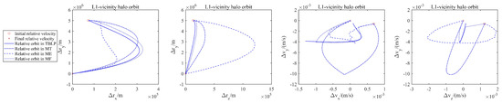
Figure 6. Relative state of Chaser and Target in L1-vicinity halo orbit.

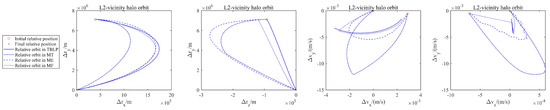
Figure 7. Relative state of Chaser and Target in L2-vicinity halo orbit.

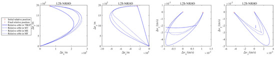
Figure 8. Relative state of Chaser and Target in L2-South Near Rectilinear Halo Orbit.

5.1.3. L2-South near Rectilinear Halo Orbit

The Near Rectilinear Halo Orbit (NRHO) is a special subset of the North and South branch halo orbits around the L1 and L2 points. The Lunar GateWay utilizes the L2-South NRHO owing to its exceptional performance, including low maintenance requirements, easy access to the lunar surface and back, and convenient departure to and arrival from deep space [36]. To asymptotically generate the L2-South NRHO from the L2 Lyapunov orbits, we construct another state correction function that assumes $\delta x=0$ (correspond to Equation (6)).

$$\begin{array}{c}\hfill \left[\begin{array}{c}\delta z\\ \delta \dot{y}\\ \delta t\end{array}\right]={\left[\begin{array}{ccc}{\Phi }_{23}& {\Phi }_{25}& \dot{y}\\ {\Phi }_{43}& {\Phi }_{45}& \ddot{x}\\ {\Phi }_{63}& {\Phi }_{65}& \ddot{z}\end{array}\right]}^{-1}\left[\begin{array}{c}0\\ \delta \dot{x}\\ \delta \dot{z}\end{array}\right]\end{array}$$

(15)

Figure 9 depicts the progressive process of the L2 Lyapunov orbit to the L2-South NRHO using these two shooting functions alternately. The ratio in parentheses indicates the orbital period to the lunar rotation period.

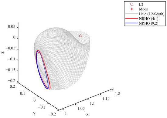
Figure 9. L2-vicinity halo orbit and L2-South NRHOs.

We employ the 9:2 lunar synodic resonance NRHO with 3250 km periapsis and 6.562 days period, the same as the Lunar GateWay. Assuming the Chaser is at apoapsis at the start time, the rendezvous will occur after 0.25 halo orbital periods, given that the Target has a phase advance of 12.5 degrees. Table 2 and Table 3 demonstrate that the use of low-thrust propulsion, as compared to the Three Body Lambert Problem (TBLP), also known as the two-impulse rendezvous, reduces fuel consumption by 42.36% to 84.62%. Additionally. the low-thrust control strategy affects the final mass, which is often inversely correlated with the rendezvous time.

Table 2. Rendezvous time comparison of three low-thrust rendezvous results to impulsive maneuver.

Orbit	L1-Halo	L2-Halo	NRHO (9:2)
MT problem	1.7235 day	2.1140 day	1.3769 day
ME problem	2.9975 day	3.7275 day	1.6405 day
MF problem	2.9975 day	3.7275 day	1.6405 day
TBLP	2.9975 day	3.7275 day	1.6405 day

Table 3. Fuel consumption comparison of three low-thrust rendezvous results to impulsive maneuver.

Orbit	L1-Halo	L2-Halo	NRHO (9:2)
MT problem	0.95 kg	1.17 kg	0.76 kg
ME problem	0.53 kg	0.47 kg	0.57 kg
MF problem	0.28 kg	0.33 kg	0.51 kg
TBLP	1.82 kg	2.03 kg	2.50 kg

5.2. Computational Efficiency and Solution Optimality

Low-thrust trajectory optimization problems often encounter two main challenges: initial value sensitivity and result optimality. To address the sensitivity issue, heuristic algorithms are often employed to provide initial value estimates. The Indirect Shooting Method (ISM) is then applied to obtain the optimal solution. Particle Swarm Optimization (PSO) [37] and ISM based on random initial costate [38] are two common initial value estimation algorithms used to solve the trajectory optimization problem.

Following Section 5.1, we maintain the dynamics parameter and thrust configuration. We then utilize these two algorithms to solve three typical low-thrust rendezvous problems in three cislunar halo orbits. The simulations were conducted using an AMD Ryzen5-5600H CPU @3.3 GHz with 16 GB RAM (designed by Advanced Micro Devices, Inc, located in Santa Clara, CA, USA) and were performed independently 10 times. Tolerance: Stage 1 (MT/ME problems): ${10}^{-5}$; Stage 2 (MF problem): ${10}^{-15}$. RPM Settings: Initial mesh: 10 intervals; collocation points per interval: 15 (Legendre-Gauss-Radau nodes). SQP Algorithm: Maximum iterations: 50; gradient threshold: ${10}^{-10}$. The CPU runtime was calculated using tic-toc in MATLAB R2021b software, as illustrated in Figure 10, and the fuel consumption result is displayed in Figure 11.

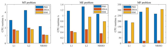
Figure 10. Computation time of the three algorithms.

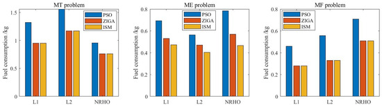
Figure 11. Fuel consumption of the three algorithms.

The PSO algorithm consumes significant computational resources and has a low convergence speed, specifically in the minimum fuel problem; this is due to the constant generation of new and different information by the particles, as well as frequent information exchange. Additionally, the PSO algorithm may generate suboptimal solutions owing to new information in the vicinity of the final generation. Conversely, the ISM algorithm produces optimal results using Newton’s iteration for optimization along the gradient direction. However, the initial costate is highly sensitive, which can lead to non-convergence and require more trial-and-error with different random initial guesses. In the most sensitive minimum fuel problem, the ISM algorithm may require more computational time compared to the PSO algorithm.

The standard indirect shooting method uses costate random initial guesses, and the computation time and convergence rate are subject to a certain degree of uncertainty. In the selected problems, the initial costate sensitivity of the MT-ME-MF problem is increasingly high, and its computational efficiency gradually decreases compared to the other two algorithms. However, the obtained solution is generally optimal owing to the application of the Pontryagin minimum principle.

As shown in Table 4, ZIGA achieves 100% convergence, outperforming PSO (80.7%) and ISM (30.2%). When the tolerance is tightened to ensure solution accuracy, ZIGA’s convergence time only increases by 15.1%, much lower than ISM’s 40.5%, demonstrating its strong robustness to tolerance variations. These results are included in the revised manuscript. Additionally, detailed benchmarking against other methods are as follows: Memory Usage: ZIGA (≈200 MB) < ISM (≈300 MB) < PSO (≈350 MB) (measured during 10 independent runs). Solution Stability: The standard deviation of fuel consumption for ZIGA is 0.02 kg, compared to 0.08 kg for PSO and 0.1 kg for ISM, indicating ZIGA’s solutions are more stable. Terminal Constraint Violation: ZIGA’s Cst (${10}^{-6}$) is an order of magnitude smaller than PSO’s (≈${10}^{-5}$) and ISM’s (≈${10}^{-5}$), confirming better solution quality.

Table 4. Convergence performance comparison of three algorithms (1000 independent simulations).

Algorithm	Convergence Rate (%)	Number of Failed Runs	Time Increase (%) a
ZIGA	100	0	15.1
PSO	80.7	193 kg	28.3
ISM	30.2	698	40.5

^a Note: Convergence time increase when tolerance decreases from ${10}^{-5}$ to ${10}^{-15}$.

The ZIGA proposed in this paper can obtain the optimal solution in MT and MF problems. The solution to the ME problem is not optimal; however, the requirement for optimality is generally not high because the objectives of orbital design typically focus on time or fuel, and the ME problem serves only as an intermediate auxiliary solution for solving the MF. In terms of computation time, ZIGA performed best in the most complex MF problems, demonstrating the algorithm’s strong robustness.

A comparison of the three algorithms reveals that although the PSO algorithm overcame the sensitivity problem, it had long runtime and non-optimal solutions. The ISM algorithm performed the best in the MT problem but had convergence issues in the ME and MF problems. The ZIGA method produced optimal results in the MF problems with much shorter running times than ISM and PSO. All independent runs of ZIGA converged in about 2 s for the MT problem, 0.5 s for the ME problem, and 15 s for the MF problem. Therefore, the ZIGA is suitable for obtaining the optimal solution to the low-thrust minimum-fuel rendezvous problem in the cislunar halo orbits and overcoming the convergence problem.

5.3. Initial Costate Estimation

In this section, we analyze Stage 2 of ZIGA, especially the homotopic process from the minimum-energy problem to the minimum-fuel problem. This process accurately estimates the initial costate of the ME problem and uses it as the initial guess for the costate of the MF problem, thereby reducing the initial value sensitivity of the MF problem. We start with the costate mapping result of the min-energy problem, the homotopic process used the SQP algorithm to optimize the parameters $[{\mathit{\lambda }}_r,{\mathit{\lambda }}_v,{\lambda }_m]$ from $ϵ=1$ to $ϵ=0$ with Equation (14). Notably, the horizontal axis in Figure 10 uses the opposite values of certain costates to use a logarithmic vertical axis.

5.3.1. Homotopy Step Size Sensitivity

Justification for Equation (14): We compared the fixed step size of Equation (14) with an adaptive step size (step size halved when constraint error > ${10}^{-6}$). The adaptive step size only reduces convergence time by 5% but increases computational complexity (due to real-time error monitoring). Since Equation (14) already ensures convergence (constraint error < ${10}^{-6}$ in all iterations) with lower complexity, it is selected as the homotopic step size scheme.

Sensitivity to Critical Parameters: We further tested the sensitivity of ZIGA to thrust magnitude (20 mN, 30 mN, 40 mN) and rendezvous duration (0.2T, 0.25T, 0.3T, where T is the orbital period). The fuel consumption variation of ZIGA is less than 3% under all test conditions, confirming its robustness to key mission parameters.

5.3.2. Comparison of Estimation Accuracy

We compared several algorithms for estimating the initial costate and summarized the results in Table 5 and Table 6. The table includes the estimated costate ($\mathit{\lambda }\left(t_0\right)$), the relative error (RE), and the terminal constraint violations (Cst). Opt denotes the optimal value of the initial costate values. Because the initial costate obtained by the standard ISM mentioned earlier was determined through random guessing, it is not used for comparison in this context. Among these methods, the particle swarm algorithm directly optimizes the initial costate. Shape-based methods (FFS [39] and IPM [40]) optimize the control law and solve for the costate through state-costate mapping. In this paper, ZIGA optimizes the state variables and control variables and obtains the initial costate estimation through the costate mapping process. The comparison between algorithms shows that the relative estimation errors of the Finite Fourier Series (FFS) and Inverse Polynomial Method (IPM) based on the shape-based method are the highest, generally exceeding 40%. The estimation errors of the particle swarm algorithm range from 30% to 40%. However, ZIGA can maintain low constraint violations while significantly reducing the initial costate estimation error. Especially in NRHO rendezvous scenarios, the initial costate estimation error is less than 10%. The computational results for the three different orbits indicate that the ZIGA’s costate estimates are generally lower than those of L1-halo and L2-halo, which may be attributed to the NRHO’s greater stability and the fact that the dynamics near the NRHO’s apolune exhibit linear behavior.

Table 5. Initial costate of different algorithms.

Orbit	Algorithm	$\mathit{\lambda }$$\left({\mathit{t}}_0\right)$
	PSO	[1.04 × ${10}^{-3}$, 1.27 × ${10}^{-2}$, 5.43 × ${10}^{-4}$, −1.39 × ${10}^{-4}$, 2.04 × ${10}^{-3}$, 6.96 × ${10}^{-4}$, 8.67 × ${10}^{-5}$]
	FFS	[5.28 × ${10}^{-5}$, 8.23 × ${10}^{-3}$, 2.90 × ${10}^{-3}$, −1.07 × ${10}^{-4}$, 3.52 × ${10}^{-3}$, 1.40 × ${10}^{-4}$, 1.94 × ${10}^{-4}$]
L1-halo	IPM	[1.22 × ${10}^{-3}$, 4.28 × ${10}^{-3}$, 1.99 × ${10}^{-3}$, −7.47 × ${10}^{-5}$, 3.98 × ${10}^{-3}$, 1.67 × ${10}^{-4}$, 4.9 × ${10}^{-5}$]
	ZIGA	[7.82 × ${10}^{-4}$, 9.83 × ${10}^{-3}$, 1.79 × ${10}^{-3}$, −1.22 × ${10}^{-4}$, 2.61 × ${10}^{-3}$, 1.59 × ${10}^{-3}$, 1.12 × ${10}^{-4}$]
	Opt.	[9.55 × ${10}^{-4}$, 1.01 × ${10}^{-2}$, 1.94 × ${10}^{-3}$, −1.39 × ${10}^{-4}$, 2.69 × ${10}^{-3}$, 1.33 × ${10}^{-3}$, 1.31 × ${10}^{-4}$]
	PSO	[3.01 × ${10}^{-3}$, 5.61 × ${10}^{-3}$, −1.33 × ${10}^{-3}$, 2.38 × ${10}^{-4}$, 5.51 × ${10}^{-4}$, −2.28 × ${10}^{-4}$, 1.54 × ${10}^{-4}$]
	FFS	[5.69 × ${10}^{-3}$, 2.80 × ${10}^{-4}$, −2.36 × ${10}^{-4}$, 8.05 × ${10}^{-4}$, 6.35 × ${10}^{-3}$, −4.06 × ${10}^{-5}$, 1.54 × ${10}^{-4}$]
L2-halo	IPM	[8.37 × ${10}^{-3}$, 7.75 × ${10}^{-3}$, −4.41 × ${10}^{-5}$, 4.55 × ${10}^{-5}$, 9.17 × ${10}^{-4}$, −1.17 × ${10}^{-3}$, 1.45 × ${10}^{-4}$]
	ZIGA	[4.75 × ${10}^{-3}$, 8.18 × ${10}^{-3}$, −8.94 × ${10}^{-4}$, 1.99 × ${10}^{-4}$, 3.42 × ${10}^{-3}$, −5.78 × ${10}^{-4}$, 1.57 × ${10}^{-4}$]
	Opt.	[4.74 × ${10}^{-3}$, 8.67 × ${10}^{-3}$, −1.09 × ${10}^{-3}$, 4.70 × ${10}^{-4}$, 3.62 × ${10}^{-3}$, −7.30 × ${10}^{-4}$, 1.73 × ${10}^{-4}$]
	PSO	[9.66 × ${10}^{-3}$, 3.61 × ${10}^{-2}$, −5.74 × ${10}^{-2}$, 4.78 × ${10}^{-4}$, 9.71 × ${10}^{-4}$, −1.46 × ${10}^{-2}$, 3.15 × ${10}^{-4}$]
	FFS	[1.74 × ${10}^{-2}$, 1.15 × ${10}^{-2}$, −9.74 × ${10}^{-3}$, 1.65 × ${10}^{-3}$, 1.10 × ${10}^{-2}$, −2.04 × ${10}^{-2}$, 8.05 × ${10}^{-4}$]
NRHO (9:2)	IPM	[2.07 × ${10}^{-2}$, 3.61 × ${10}^{-2}$, −3.84 × ${10}^{-2}$, 6.17 × ${10}^{-4}$, 9.02 × ${10}^{-3}$, −2.79 × ${10}^{-4}$, 3.49 × ${10}^{-4}$]
	ZIGA	[1.33 × ${10}^{-2}$, 3.58 × ${10}^{-2}$, −5.76 × ${10}^{-2}$, 1.17 × ${10}^{-3}$, 7.06 × ${10}^{-3}$, −1.34 × ${10}^{-2}$, 6.26 × ${10}^{-4}$]
	Opt.	[1.50 × ${10}^{-2}$, 4.27 × ${10}^{-2}$, −5.94 × ${10}^{-2}$, 1.22 × ${10}^{-3}$, 8.34 × ${10}^{-3}$, −1.36 × ${10}^{-2}$, 6.21 × ${10}^{-4}$]

Table 6. Comparison of algorithms for costate initialization.

Orbit	Algorithm	RE (%)	Cst
	PSO	30.54%	1.04 × ${10}^{-3}$
	FFS	50.61%	7.56 × ${10}^{-6}$
L1-halo	IPM	47.36%	8.59 × ${10}^{-6}$
	ZIGA	11.09%	9.86 × ${10}^{-6}$
	Opt.	-	9.79 × ${10}^{-6}$
	PSO	43.91%	3.52 × ${10}^{-3}$
	FFS	63.98%	8.45 × ${10}^{-6}$
L2-halo	IPM	60.74%	7.16 × ${10}^{-6}$
	ZIGA	16.73%	7.65 × ${10}^{-6}$
	Opt.	-	8.26 × ${10}^{-6}$
	PSO	37.15%	6.05 × ${10}^{-3}$
	FFS	45.69%	8.64 × ${10}^{-6}$
NRHO (9:2)	IPM	41.19%	7.49 × ${10}^{-6}$
	ZIGA	7.39%	8.19 × ${10}^{-6}$
	Opt.	-	8.24 × ${10}^{-6}$

The difference between the two results of costate at $ϵ=1$ (denote by pink diamond and red stars) in Figure 12 denotes the non-optimality of the discrete costate in the costate mapping process; however, it provides a valuable initial guess to start the homotopic process. The costate slowly changes in the homotopic process and obtains the optimal value at the final point $ϵ=0$, which denotes the optimal solution of the MF problem. We can obtain the optimal control law and relative state history by integrating the dynamic equation and the costate dynamic from $t_0$ to $t_f$ using the initial state and costate. For instance, Figure 13 illustrates the history of the control law, chaser mass, and relative state on the NRHO (9:2).

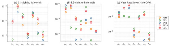
Figure 12. Initial costate estimation of minimum-energy problem.

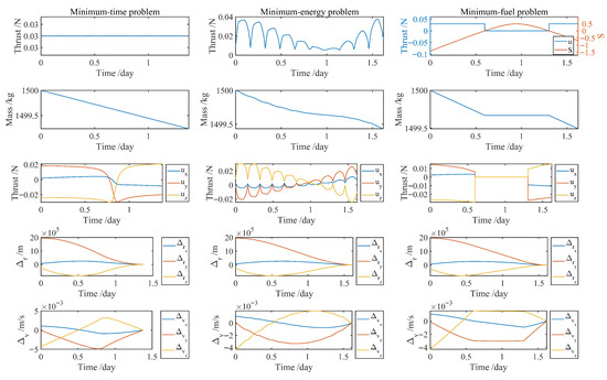
Figure 13. Results of three rendezvous problem on NRHO (9:2).

Figure 13 illustrates all three low-thrust rendezvous modes with different trajectories. The problem of MT sets the minimum limit for the rendezvous time, whereas the ME problem acts as a transitional step towards solving the MF problem. All three problems rendezvous successfully at the final time with different optimal control laws. In the MT problem, the engine operates with maximum thrust continually to get the minimum rendezvous time. In the ME problem, the control vector is interpolated using the continuous Legendre polynomials in Stage 1 of ZIGA; the thrust amplitudes are always greater than zero. We obtain the bang-bang control law by solving the two-point boundary value problem constructed by the MF problem, as shown in Figure 13. Chaser’s control vector only worked 0.9166 days, which led to the minimum fuel consumption.

6. Conclusions

The manuscript proposes a trajectory optimization method for the low-thrust problem. The method does not require any initial guess and greatly reduces the costate sensitivity. The ZIGA shows high computational efficiency and initial costate estimation accuracy when applied to the low-thrust rendezvous problem on three typical cislunar orbits. In the minimum-fuel problem, utilizing a homotopic process in Stage 2 of ZIGA reduces the difficulty of obtaining the numerical solution and converges to the optimal result. A comparison of other initial value guess algorithms shows that this method has a much lower computational burden and greater optimality. Simulation results show that low-thrust propulsion reduces fuel consumption by 42.36% to 84.62% in the established scenario compared to traditional impulsive maneuvers.

ZIGA is based on Pontryagin’s Minimum Principle and uses a homotopic process to gradually approach the optimal solution of the MF problem. While strict mathematical proof of global optimality remains challenging, our 10 independent simulations across three orbital scenarios show that ZIGA’s fuel consumption is consistently lower than the optimal results of PSO and ISM, with terminal constraint violations (Cst) < ${10}^{-5}$. Thus, ZIGA can be considered an engineering-level approximate global optimal solution.

Future work will focus on analyzing theoretical error boundaries, improving algorithm performance, and expanding applications. Conducting rigorous analysis on the convergence properties of ZIGA and the error bounds of the NLP-to-costate mapping and developing adaptive homotopic strategies or costate correction mechanisms can enhance ZIGA’s performance. Research on integrating ZIGA and other optimization techniques can enhance algorithms, such as sequential convex optimization for real-time applications. In addition, ZIGA can also be applied to more complex mission scenarios such as multi-spacecraft cooperative trajectory planning, asteroid rendezvous with irregular gravity fields, or low-thrust transfers in multi-body systems (e.g., Trojan asteroid belt).

References

- Li, C.; Zuo, W.; Wen, W.; Zeng, X.; Gao, X.; Liu, Y.; Fu, Q.; Zhang, Z.; Su, Y.; Ren, X.; et al. Overview of the Chang’e-4 Mission: Opening the Frontier of Scientific Exploration of the Lunar Far Side. Space Sci. Rev. 2021, 217, 35. [Google Scholar] [CrossRef]
- Coderre, K.M.; Edwards, C.; Cichan, T.; Richey, D.; Shupe, N.; Sabolish, D.; Ramm, S.; Perkes, B.; Posey, J.; Pratt, W. Concept of Operations for the Gateway. In Proceedings of the 2018 SpaceOps Conference, Marseille, France, 28 May–1 June 2018. [Google Scholar] [CrossRef]
- Singh, S.; Junkins, J.; Anderson, B.; Taheri, E. Eclipse-Conscious Transfer to Lunar Gateway Using Ephemeris-Driven Terminal Coast Arcs. J. Guid. Control Dyn. 2021, 44, 1972–1988. [Google Scholar] [CrossRef]
- Gerding, R.B. Rendezvous equations in the vicinity of the second libration point. J. Spacecr. Rocket. 1971, 8, 292–294. [Google Scholar] [CrossRef]
- Luquette, R.J.; Sanner, R.M. Linear state-space representation of the dynamics of relative motion, based on restricted three body dynamics. Collect. Tech. Pap.-AIAA Guid. Navig. Control Conf. 2004, 1, 353–361. [Google Scholar] [CrossRef][Green Version]
- Jones, B.L.; Bishop, R.H. Rendezvous targeting and navigation for a translunar halo orbit. J. Guid. Control Dyn. 1994, 17, 1109–1114. [Google Scholar] [CrossRef]
- Franzini, G.; Innocenti, M. Relative Motion Dynamics in the Restricted Three-Body Problem. J. Spacecr. Rocket. 2019, 56, 1322–1337. [Google Scholar] [CrossRef]
- Murakami, N.; Yamanaka, K. Trajectory design for rendezvous in lunar Distant Retrograde Orbit. In Proceedings of the 2015 IEEE Aerospace Conference, Big Sky, MT, USA, 7–14 March 2015; pp. 1–13. [Google Scholar] [CrossRef]
- Franzini, G.; Innocenti, M.; Casasco, M. An Adjoint-Based Method for Continuous-Thrust Relative Maneuver Computation in the Restricted Three-Body Problem. In Proceedings of the 2021 American Control Conference (ACC), New Orleans, LA, USA, 25–28 May 2021; pp. 4276–4281. [Google Scholar] [CrossRef]
- Shirazi, A.; Ceberio, J.; Lozano, J.A. Spacecraft trajectory optimization: A review of models, objectives, approaches and solutions. Prog. Aerosp. Sci. 2018, 102, 76–98. [Google Scholar] [CrossRef]
- Zuehlke, D.; Tiwari, M.; Jebari, K.; Kidambi, K.B. Rendezvous and Proximity Operations in Cislunar Space Using Linearized Dynamics for Estimation. Aerospace 2023, 10, 674. [Google Scholar] [CrossRef]
- Roth, N.H.; Johnston-Lemke, B.; Damaren, C.J.; Zee, R.E. Formation and Attitude Control for the CanX-4 and CanX-5 Formation Flying Mission. IFAC Proc. Vol. 2011, 44, 3033–3038. [Google Scholar] [CrossRef]
- Thompson, M.R.; Forsman, A.; Chikine, S.; Peters, B.C.; Ely, T.; Sorensen, D.; Parker, J.; Cheetham, B. Cislunar Navigation Technology Demonstrations on the CAPSTONE Mission. In Proceedings of the 2022 International Technical Meeting of The Institute of Navigation, Long Beach, CA, USA, 25–27 January 2022. [Google Scholar] [CrossRef]
- Sonwalkar, N.; Matteson, E. Cislunar Explorers Redesign: Multiple, Independent Technology Demonstrations Reduce Mission Risk. In Proceedings of the AIAA SCITECH 2024 Forum, Orlando, FL, USA, 8–12 January 2024. [Google Scholar] [CrossRef]
- Foing, B.; Racca, G. The ESA SMART-1 mission to the Moon with solar electric propulsion. Adv. Space Res. 1999, 23, 1865–1870. [Google Scholar] [CrossRef]
- Steiger, C.; Romanazzo, M.; Emanuelli, P.P.; Floberghagen, R.; Fehringer, M. The Deorbiting of ESA’s Gravity Mission GOCE-Spacecraft Operations in Extreme Drag Conditions. In Proceedings of the SpaceOps 2014 Conference, Pasadena, CA, USA, 5–9 May 2014. [Google Scholar] [CrossRef]
- Ignatenko, V.; Laurila, P.; Radius, A.; Lamentowski, L.; Antropov, O.; Muff, D. ICEYE Microsatellite SAR Constellation Status Update: Evaluation of First Commercial Imaging Modes. In Proceedings of the IGARSS 2020-2020 IEEE International Geoscience and Remote Sensing Symposium, Waikoloa, HI, USA, 26 September–2 October 2020. [Google Scholar] [CrossRef]
- Wilkie, W.K. Overview of the NASA Advanced Composite Solar Sail System (ACS3) Technology Demonstration Project. In Proceedings of the AIAA Scitech 2021 Forum, Nashville, TN, USA, 11–15 January 2021. [Google Scholar] [CrossRef]
- Darby, C.L.; Hager, W.W.; Rao, A.V. Direct Trajectory Optimization Using a Variable Low-Order Adaptive Pseudospectral Method. J. Spacecr. Rocket. 2011, 48, 433–445. [Google Scholar] [CrossRef]
- Taheri, E.; Arya, V.; Junkins, J.L. Costate mapping for indirect trajectory optimization. Astrodynamics 2021, 5, 359–371. [Google Scholar] [CrossRef]
- Zhang, C.; Topputo, F.; Bernelli-Zazzera, F.; Zhao, Y.S. Low-Thrust Minimum-Fuel Optimization in the Circular Restricted Three-Body Problem. J. Guid. Control Dyn. 2015, 38, 1501–1510. [Google Scholar] [CrossRef]
- Zhang, Z.; Zhang, Y.; Xue, J.; Shi, X.; Wang, B.; Zhang, Y. Homotopic approach to the feedback solution of the orbit pursuit-evasion game. Adv. Space Res. 2025, 76, 455–468. [Google Scholar] [CrossRef]
- Meng, Y.; Zhang, H.; Gao, Y. Low-Thrust Minimum-Fuel Trajectory Optimization Using Multiple Shooting Augmented by Analytical Derivatives. J. Guid. Control Dyn. 2019, 42, 662–677. [Google Scholar] [CrossRef]
- Alvarado, K.I.; Singh, S.K. Exploration and Maintenance of Homeomorphic Orbit Revs in the Elliptic Restricted Three-Body Problem. Aerospace 2024, 11, 407. [Google Scholar] [CrossRef]
- Jiang, F.; Baoyin, H.; Li, J. Practical Techniques for Low-Thrust Trajectory Optimization with Homotopic Approach. J. Guid. Control Dyn. 2012, 35, 245–258. [Google Scholar] [CrossRef]
- Zhang, Z.; Zhang, Y.; Wang, B. Application of the hp-adaptive pseudospectral method in spacecraft orbit pursuit-evasion game. Adv. Space Res. 2024, 73, 1597–1610. [Google Scholar] [CrossRef]
- Singh, S.K.; Anderson, B.D.; Taheri, E.; Junkins, J.L. Low-Thrust Transfers to Southern L 2 Near-Rectilinear Halo Orbits Facilitated by Invariant Manifolds. J. Optim. Theory Appl. 2021, 191, 517–544. [Google Scholar] [CrossRef]
- Richardson, D.L. Analytic construction of periodic orbits about the collinear points. Celest. Mech. 1980, 22, 241–253. [Google Scholar] [CrossRef]
- Singh, S.K.; Anderson, B.D.; Taheri, E.; Junkins, J.L. Exploiting manifolds of L 1 halo orbits for end-to-end Earth–Moon low-thrust trajectory design. Acta Astronaut. 2021, 183, 255–272. [Google Scholar] [CrossRef]
- Bryson, A.E.; Ho, Y.C.; Siouris, G.M. Applied Optimal Control: Optimization, Estimation, and Control. IEEE Trans. Syst. Man Cybern. 1979, 9, 366–367. [Google Scholar] [CrossRef]
- Caillau, J.B.; Daoud, B. Minimum Time Control of the Restricted Three-Body Problem. SIAM J. Control Optim. 2012, 50, 3178–3202. [Google Scholar] [CrossRef]
- Gong, Q.; Ross, I.M.; Fahroo, F. Costate Computation by a Chebyshev Pseudospectral Method. J. Guid. Control Dyn. 2010, 33, 623–628. [Google Scholar] [CrossRef]
- Darby, C.L.; Garg, D.; Rao, A.V. Costate Estimation using Multiple-Interval Pseudospectral Methods. J. Spacecr. Rocket. 2011, 48, 856–866. [Google Scholar] [CrossRef]
- Cook, A.; Dahlke, J.; Bettinger, R.A. Preliminary Study of Employing Space-Based Mirrors for Augmented Illumination of Cislunar Resident Space Objects. In Proceedings of the AIAA SCITECH 2023 Forum, Online, 23–27 January 2023. [Google Scholar] [CrossRef]
- Singh, S.K.; Taheri, E.; Woollands, R.; Junkins, J. Mission Design for Close-Range Lunar Mapping by Quasi-Frozen Orbits. In Proceedings of the 70th International Astronautical Congress, Washington, DC, USA, 21–25 October 2019. [Google Scholar]
- Zimovan-Spreen, E.M.; Howell, K.C.; Davis, D.C. Near Rectilinear Halo Orbits and Nearby Higher-Period Dynamical Structures: Orbital Stability and Resonance Properties. Celest. Mech. Dyn. Astron. 2020, 132, 28. [Google Scholar] [CrossRef]
- Pontani, M.; Conway, B.A. Particle Swarm Optimization Applied to Space Trajectories. J. Guid. Control Dyn. 2010, 33, 1429–1441. [Google Scholar] [CrossRef]
- Barron, R.L.; Chick, C.M. Improved Indirect Method for Air-Vehicle Trajectory Optimization. J. Guid. Control Dyn. 2006, 29, 643–652. [Google Scholar] [CrossRef]
- Taheri, E.; Sowell, S. Enhanced Finite Fourier Series for Low-Thrust Trajectory design. In Proceedings of the AIAA SCITECH 2024 Forum, Orlando, FL, USA, 8–12 January 2024. [Google Scholar] [CrossRef]
- Wall, B.J.; Conway, B.A. Shape-Based Approach to Low-Thrust Rendezvous Trajectory Design. J. Guid. Control Dyn. 2009, 32, 95–101. [Google Scholar] [CrossRef]
Disclaimer/Publisher’s Note: The statements, opinions and data contained in all publications are solely those of the individual author(s) and contributor(s) and not of MDPI and/or the editor(s). MDPI and/or the editor(s) disclaim responsibility for any injury to people or property resulting from any ideas, methods, instructions or products referred to in the content. |
© 2025 by the authors. Licensee MDPI, Basel, Switzerland. This article is an open access article distributed under the terms and conditions of the Creative Commons Attribution (CC BY) license (https://creativecommons.org/licenses/by/4.0/).