Robust Vehicle Pose Estimation Through Multi-Sensor Fusion of Camera, IMU, and GPS Using LSTM and Kalman Filter

Abstract

Accurate vehicle localization remains a critical challenge due to the frequent loss or degradation of sensor data, such as from visual, inertial, and GPS sources. In this study, we present a novel localization algorithm that dynamically fuses data from heterogeneous sensors to achieve stable and precise positioning. The proposed algorithm integrates a deep learning-based visual-inertial odometry (VIO) module with a Kalman filter for global data fusion. A key innovation of the method is its adaptive fusion strategy, which adjusts feature weights based on sensor reliability, thereby ensuring optimal data utilization. Extensive experiments across varied scenarios demonstrate the algorithm’s superior performance, consistently achieving lower RMSE values and reducing position errors by 79–91% compared to four state-of-the-art baselines—even under adverse conditions such as sensor failures or missing data. This work lays the foundation for deploying robust localization systems in real-world applications, including autonomous vehicles, robotics, and navigation technologies.

1. Introduction

Pose estimation refers to the process of determining an agent’s position and orientation using various sensors, including cameras, LiDAR, GPS, and inertial measurement units. It involves calculating relative motion between sequential sensor data frames and integrating these estimates to obtain the agent’s global pose. Accurate and stable pose estimation is fundamental to numerous applications, such as autonomous driving [1,2,3], robotics [4,5,6], drones [7,8,9], AR/VR systems [10,11,12], and wearable devices [13,14,15], where precise and stable localization is critical.

Traditionally, pose estimation has been formulated as a state estimation problem under the Markov assumption, using analytical models designed for specific sensor types. Representative examples include strapdown inertial navigation systems (SINS), pedestrian dead reckoning (PDR), and various odometry-based methods such as visual odometry (VO) [16,17,18], visual-inertial odometry (VIO) [19,20,21], LiDAR odometry (LO) [22,23,24], and simultaneous localization and mapping (SLAM) [25,26,27]. While these models can achieve high accuracy under ideal conditions, their performance often deteriorates in real-world scenarios due to sensor noise, failures, or dynamic environmental changes.

To address these challenges, recent studies have increasingly turned to deep learning techniques to extract robust features directly from raw sensor data. Deep neural networks, particularly convolutional architectures, have shown strong potential in learning complex mappings from input data to motion outputs. More recently, transformer-based models [28,29,30,31,32] have further enhanced performance by capturing long-range dependencies and contextual relationships across different sensor modalities.

Despite these advances, most deep learning-based methods are designed under the assumption of ideal operating conditions, without accounting for issues such as sensor failures or missing data. In practical scenarios, events like network packet loss, sensor disconnection, or hardware degradation frequently compromise data integrity and availability. Existing fusion methods [33,34,35,36,37] typically extract features from raw sensor data using encoders and make fusion decisions without explicitly evaluating the reliability or quality of these features. This lack of reliability assessment makes them susceptible to failure under non-ideal conditions.

Recent advances in multi-sensor fusion have also focused on improving localization robustness under challenging conditions, including dynamic environments and unreliable sensor data [38,39,40]. These works further emphasize the importance of adaptive and reliable fusion strategies, which motivate the design of our method.

To overcome this limitation, we propose a novel pose estimation framework that incorporates auxiliary pose estimators into the fusion process. Each auxiliary estimator independently predicts pose based on features from a specific sensor and produces hidden latent vectors representing its intermediate processing results. These latent vectors act as implicit indicators of data quality and are used by the fusion module to assign adaptive weights to each sensor’s input. This mechanism allows the system to down-weight unreliable data sources, thereby improving tolerance to sensor failures or missing inputs.

Our system performs local pose estimation using a deep neural network that fuses visual and inertial data to predict relative motion. These local estimates are then combined with global GPS-derived position data via a Kalman filter. To address coordinate system differences between local and global sensors, we modify the neural network to incorporate the Kalman filter’s prior state estimates as additional inputs, enabling consistent and seamless fusion.

To facilitate effective model learning, we adopt a two-stage training strategy. In the first stage, the auxiliary pose estimators are trained independently until they achieve sufficient accuracy. In the second stage, the fusion module is trained while keeping the auxiliary estimators fixed, allowing it to leverage their reliable latent representations. This staged approach improves both training efficiency and model stability.

In summary, our method enables accurate and robust localization even under adverse conditions such as data loss or sensor degradation. The main contributions of this work are as follows:

• We propose an integrated localization architecture that combines local relative motion estimation and global GPS data using a deep neural network and Kalman filter, improving pose estimation accuracy and reliability.
• We introduce a novel fusion strategy that leverages latent vectors from auxiliary pose estimators to assess sensor data reliability, enabling robust performance in the presence of sensor failures or missing data.
• We develop a staged training approach that enhances fusion performance by ensuring the module operates on high-quality inputs from pretrained auxiliary networks.
• We validate our method through extensive experiments, demonstrating stable performance in challenging scenarios. On KITTI sequences 07 and 10, our method reduced the average position RMSE by 79–91% compared to four state-of-the-art baselines (VS VIO, Hard VIO, Soft VIO, and VINet), confirming its effectiveness for real-world deployment in autonomous systems.

2. Proposed Robust Vehicle Pose Estimation Algorithm

2.1. Overall System Architecture

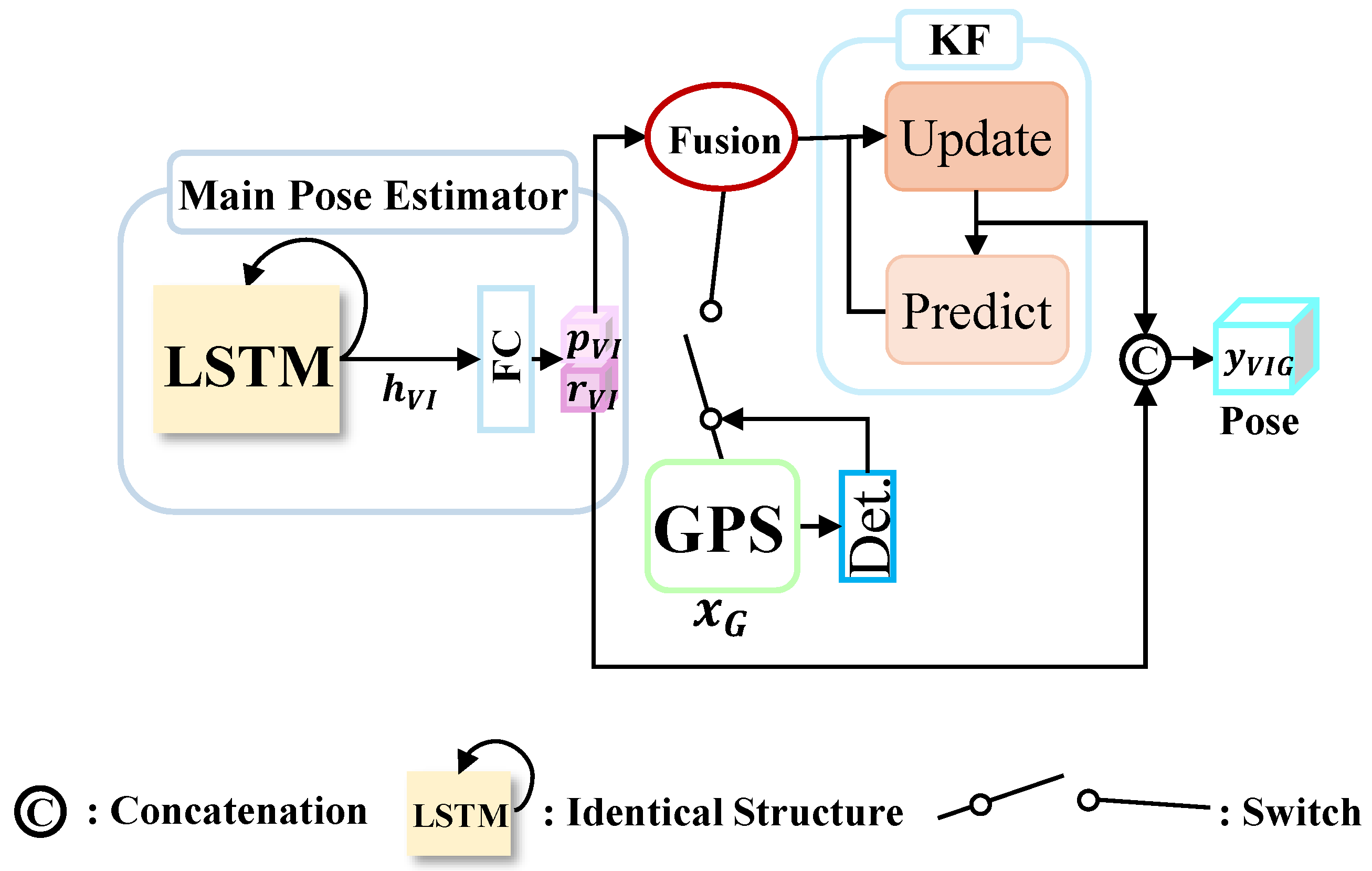
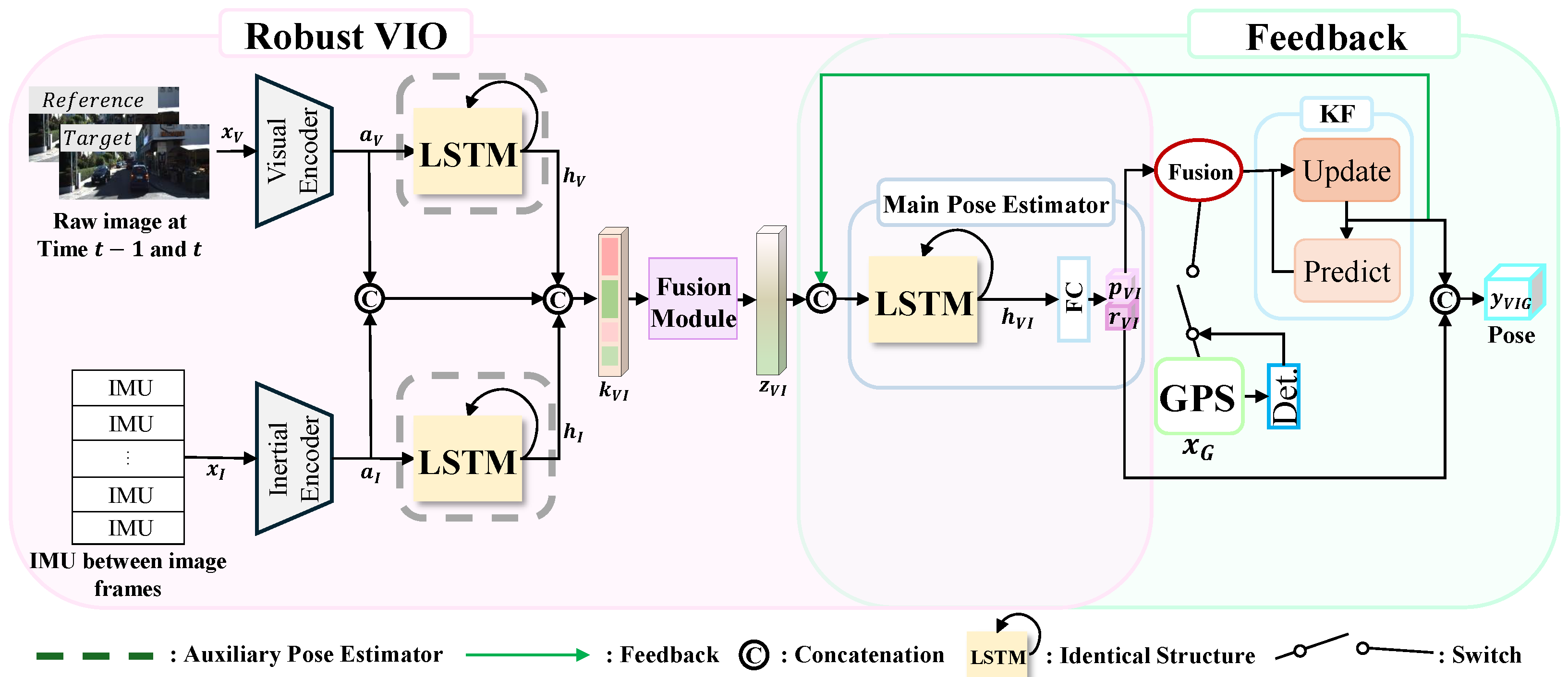
Figure 1 illustrates overview of the proposed method. As shown in Figure 1, overall system architecture of the robust vehicle pose estimation algorithm is designed as an integrated framework to efficiently fuse diverse sensor data for robust and accurate localization. Unlike conventional methods that uniformly process all sensor data, this architecture employs a modular approach tailored to the specific characteristics of each sensor. Local data-driven sensors, such as visual and inertial sensors, are processed through a deep neural network to estimate relative motion, while global sensors like GPS are integrated using a Kalman filter for absolute positioning. This separation allows the system to effectively combine fine-grained motion details from local sensors with reliable global positional information from GPS.

Figure 1. Overview of Proposed Method.

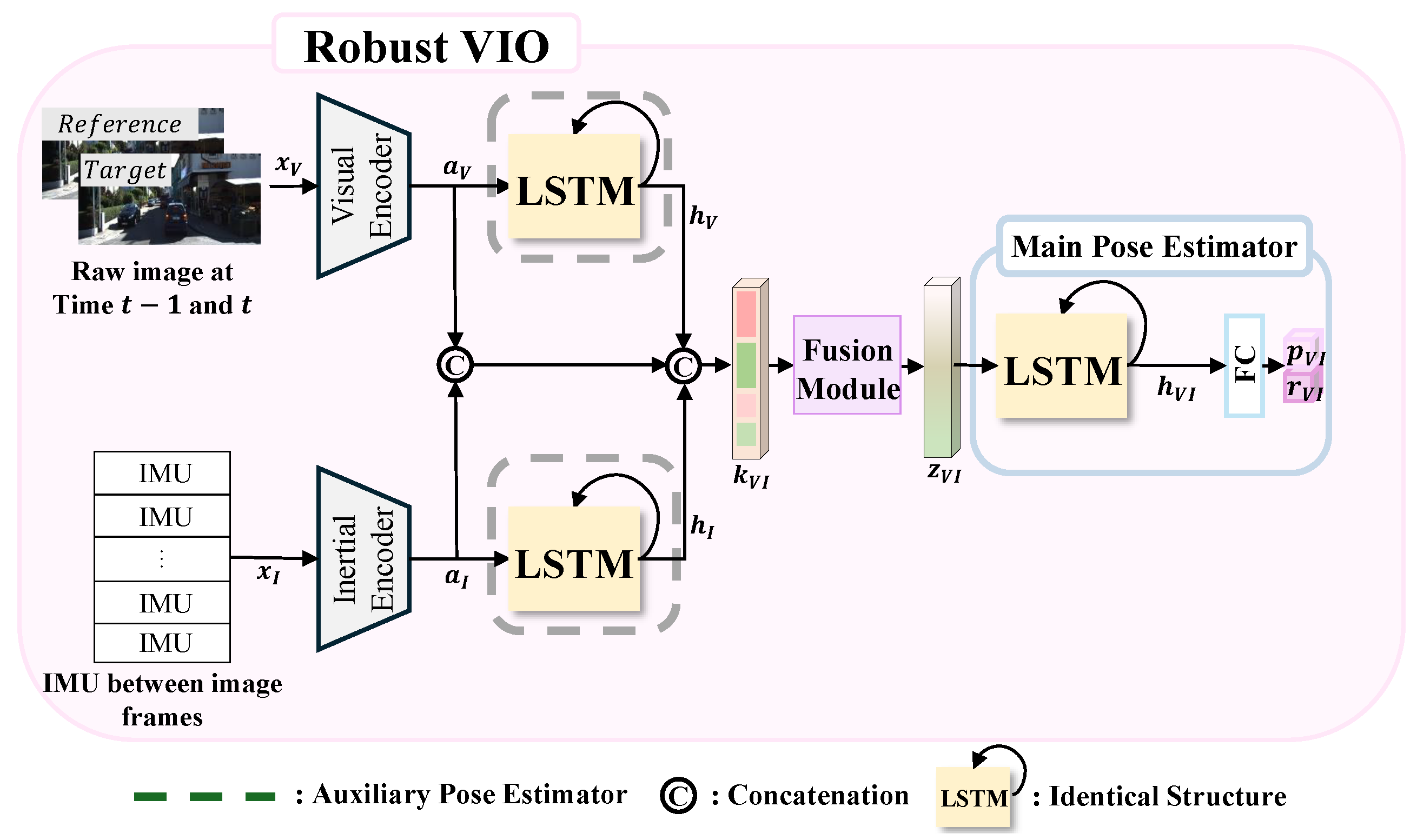
Raw data from visual, inertial, and GPS sensors flows through the system in a structured manner. Visual and inertial data are first fed into the VIO module, where dedicated feature encoders convert raw inputs into high-dimensional feature vectors that capture meaningful spatial and temporal patterns. These feature vectors are then passed to the fusion module, which dynamically adjusts their weights based on the assessed reliability of each sensor. The weighted features are processed by an LSTM-based pose estimator that models temporal dependencies to predict the local pose. Two LSTM modules process visual and inertial features separately, generating pose outputs and hidden state vectors, while another LSTM module processes fused features (visual and inertial) to predict position and orientation.

All three LSTM modules follow the same two-layer unidirectional architecture, differing only in their input features (visual, inertial, or fused). This architecture was intentionally designed to ensure structural compatibility among modules—since the hidden latent vectors produced by the two auxiliary pose estimators are integrated through the fusion module and subsequently processed by the main pose estimator—thereby facilitating stable information transfer and efficient joint optimization.

The hidden state vectors provide reliability cues that guide adaptive fusion. The pose estimator outputs position and orientation components separately: orientation is directly included in the system’s final output, while position undergoes further refinement for enhanced accuracy.

For positional data handling, the system includes a detector responsible for evaluating GPS data availability. Figure 2 illustrates the architecture of the proposed detector. In Figure 2, when all GPS values are zero, indicating missing data, the detector assigns a weight $w_G$ of 0. In contrast, when GPS data is present and valid, the weight $w_G$ is set to 0.5, signaling full reliability. This weight is then used to fuse the positional output from the VIO module with the GPS position to form the observation vector o. By dynamically adjusting $w_G$ based on GPS availability, the detector prevents unreliable GPS data from corrupting the fusion process, while seamlessly integrating reliable GPS information.

$$\begin{array}{c}\hfill \begin{array}{cc}\hfill p& =(1-w_G)·p_{VI}+w_G·p_G,\hfill \\ \hfill o& ={[p_x,p_y,p_z]}^T.\hfill \end{array}\end{array}$$

(1)

where p is the fused position vector, and $w_G$ weights the VIO output position $p_{VI}$ and the GPS position $p_G$ dynamically. The observation vector $o={[p_x,p_y,p_z]}^T$ consists of the position coordinates fed into the Kalman filter.

Figure 2. Detector for Dynamic GPS Data Availability.

The observation vector o is input into the Kalman filter’s update cycle, which operates in two stages: prediction and update. During prediction, the filter estimates the current state and covariance matrix based on the previous state. In the update stage, it incorporates the observation vector to refine these estimates, correcting any deviations and improving accuracy. This iterative process enables the Kalman filter to maintain reliable position estimates even when GPS data is missing or unreliable. By adaptively integrating observation data, the system achieves robust localization across diverse and challenging sensor conditions.

The system’s final localization output combines position estimates from the Kalman filter with orientation estimates from the VIO module. This architecture ensures each module performs its specialized function while working synergistically. The detector continuously assesses GPS data reliability to exclude unreliable inputs, preventing distortion of the observation vector. Simultaneously, the fusion module evaluates visual and inertial data quality, dynamically adjusting their contributions to optimize localization accuracy. By effectively integrating detailed local motion from the VIO module with global positioning from GPS, the Kalman filter produces precise position estimates, enhancing the overall adaptability of the system under varying conditions.

2.2. Robust VIO: Fusion of Multi-Sensor Data for Robust Localization

In this section, we describe the proposed Robust VIO module. Figure 3 illustrates the overall architecture of the fusion of multi-sensor data. As shown in Figure 3, the proposed fusion of multi-sensor data for robust localization is largely composed of a Feature Encoder, Fusion Module, Temporal Modeling, and Pose Estimator. The specific configuration and learning method of each module are described as follows.

Figure 3. Robust VIO Architecture: Fusion of Multi-Sensor Data for Robust Localization.

2.2.1. Feature Encoder

Visual Feature Encoder

The visual feature encoder is designed to extract latent representations from two consecutive monocular images to capture the relative motion of a mobile agent. To ensure that the model learns geometrically meaningful features—rather than overfitting to texture, appearance, or scene context—we employ FlowNetSimple, a convolutional neural network optimized for optical flow prediction. FlowNetSimple is particularly effective at capturing pixel displacement between image frames, making it well-suited for estimating motion.

The architecture comprises nine convolutional layers, with receptive field sizes progressively decreasing from 7 × 7 to 5 × 5 and finally to 3 × 3. This multiscale structure allows the network to extract spatial information at various resolutions and to learn hierarchical features. To improve computational efficiency, the first six layers apply a stride of 2, reducing the spatial dimensions of the feature maps. Each convolutional layer—except the last—is followed by a ReLU activation to introduce non-linearity into the model. The final feature map output from the last convolutional layer is used as the visual feature representation, defined as:

$$\begin{array}{c}\hfill a_V=f_{\mathrm{visual}}\left(x_V\right)\end{array}$$

(2)

These extracted visual features are then fused with features from inertial sensors to support accurate and robust state estimation. The multi-sensor fusion significantly ensures consistent system performance.

Inertial Feature Encoder

The inertial feature encoder plays a crucial role in extracting motion information of a mobile agent by processing high-frequency data from an inertial measurement unit (IMU). Unlike image data, which is typically sampled at about 10 Hz, inertial data is collected at a much higher frequency (around 100 Hz), allowing for the effective capture of fine-grained temporal dependencies between consecutive measurements. To leverage this temporal information, we design the inertial encoder using Conv1D layers, which are particularly well-suited for capturing local temporal patterns in sequential data while maintaining computational efficiency in processing high-frequency signals.

The encoder consists of three Conv1D layers with 64, 128, and 256 filters, respectively. Each layer is followed by batch normalization and a LeakyReLU activation function to improve non-linearity and enhance representational capacity. A final fully connected layer generates a 256-dimensional feature vector, as shown in the equation:

$$\begin{array}{c}\hfill a_I=f_{\mathrm{inertial}}\left(x_I\right)\end{array}$$

(3)

where $x_I$ represents the sequence of inertial measurements recorded between two consecutive image frames. The resulting feature vector $a_I$ captures temporal variations in acceleration and angular velocity, providing detailed insight into the mobile agent’s motion. This vector is later fused with visual features to support accurate pose estimation.

The Conv1D-based architecture allows for efficient processing of high-frequency inertial signals, capturing rapid movements and vibrations that may not be easily detectable through visual data alone.

2.2.2. Temporal Modeling and Pose Estimation

Effectively modeling temporal dependencies in sequential data is vital for accurate pose estimation. While traditional methods often rely on state-space models to describe the evolution of system states over time, our approach utilizes an LSTM network to learn temporal patterns directly from the data.

To balance modeling capacity and computational efficiency, we adopt a two-layer unidirectional LSTM as the main pose estimator. The unidirectional LSTM is well-suited for real-time applications, where future data is not yet available and efficient sequential processing is essential. Although bidirectional LSTMs can leverage both past and future contexts, they introduce additional latency and are less practical for real-time systems.

In contrast to conventional deep learning-based VIO models, our framework includes an auxiliary pose estimator in addition to the main estimator. The auxiliary estimator processes individual sensor features independently, providing complementary pose estimates. This dual-estimator setup improves fault tolerance by offering independent assessments of visual and inertial data, thereby improving the reliability and stability of the final pose estimation.

Auxiliary Pose Estimator

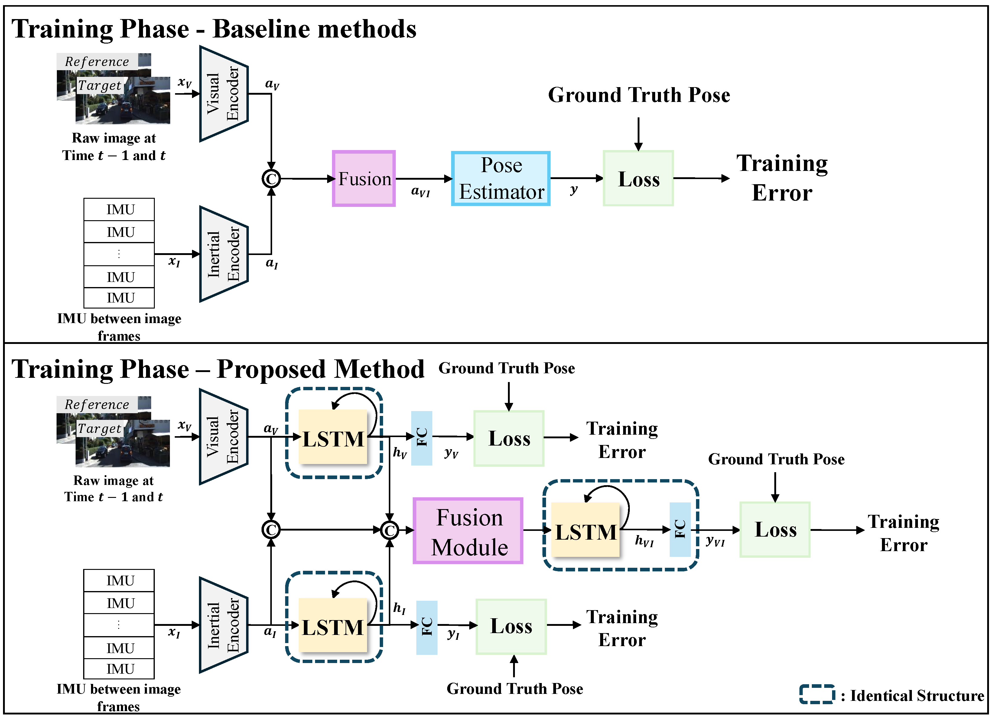
The auxiliary pose estimators independently process each sensor’s features before they are passed to the main pose estimator. Figure 4 shows a comparison of the existing methods and the proposed approach using the auxiliary pose estimator. As shown in Figure 4, the proposed approach provides essential information to the fusion module for determining the feature weights.

Figure 4. Comparison of Other Methods and Proposed Approach with Auxiliary Pose Estimator.

At each time step t, the auxiliary pose estimator receives the individual sensor feature $a_t$ along with the previous hidden state $h_{t-1}$ as inputs, enabling it to learn dynamic dependencies and interactions within the sequence. Since this estimation occurs prior to feature fusion, the resulting hidden state $h_t$ retains important information specific to the current sensor input, which is essential for accurate and timely pose estimation. Specifically, $h_t$ captures past interactions with the current sensor modality and acts as a valuable reference for evaluating the reliability of each sensor.

In this setup, each sensor feature $a_t$, whether from the visual or inertial encoder, is passed into an LSTM network, where it is combined with the hidden state $h_{t-1}$ to predict the pose transformation $y_t$. The resulting hidden state $h_t$ serves as a latent vector representing the temporal context at the current time step. This latent vector is then utilized in the fusion module to determine the weight of each sensor’s contribution. The process is mathematically expressed as:

$$\begin{array}{c}\hfill [y_t,h_t]=\mathrm{RNN}(a_t,h_{t-1})\end{array}$$

(4)

where $a_t$ denotes either the visual sensor feature $a_V$ or the inertial sensor feature $a_I$, and the output $[y_t,h_t]$ consists of the predicted pose transformation $y_t$ and the updated hidden state vector $h_t$. The hidden state $h_t$ acts as the hidden latent vector for the current time step, encapsulating temporal information that is utilized by the fusion module to determine the reliability weights of the sensor features. The latent vectors $h_V$ and $h_I$ are the outputs of the auxiliary pose estimators corresponding to visual and inertial inputs, respectively. Following the LSTM layer, an FC layer serves as a regressor to estimate the pose transformation $y_t$ based on the learned features.

Main Pose Estimator

In traditional approaches, the pose at each time step t is estimated using a combined feature representation $z_t$ along with the previous hidden state $h_{t-1}$. In our framework, however, we move beyond uniformly fusing all sensor inputs. Instead, we construct a deep neural network that separately integrates local sensors such as visual and inertial sensors that capture relative motion between consecutive frames. For absolute positioning information from global sources like GPS, we incorporate a Kalman filter to fuse this data with local pose estimates, facilitating a hybrid localization strategy.

One major challenge in sensor fusion is the discrepancy between coordinate frames of local sensors (visual/inertial) and GPS. To resolve this, we design a feedback structure where the local pose estimator receives the Kalman filter’s estimate from the previous time step as a recursive input. This mechanism mitigates frame inconsistencies and facilitates effective fusion between local and global data sources.

Figure 5 illustrates the proposed feedback structure for resolving coordinate frame discrepancy between visual, inertial sensors and GPS. In Figure 5, the feedback structure operates differently during training and inference. During training, where GPS data and thus Kalman filter outputs are unavailable, the previous output of the neural network $y_{t-1}$ is used as input. In inference, the previous state estimate $s_{t-1}$ from the Kalman filter is used instead. This dual-mode feedback structure is captured by the following equations:

$$\begin{array}{c}\hfill y_t=\mathrm{RNN}(z_t,h_{t-1},y_{t-1})\end{array}$$

(5)

during inference, the feedback model is represented as follows:

$$\begin{array}{c}\hfill y_t=\mathrm{RNN}(z_t,h_{t-1},s_{t-1})\end{array}$$

(6)

The LSTM network, followed by an FC layer, functions as a regressor to predict the pose transformation $y_t$. This architecture enables precise estimation of the mobile agent’s position and orientation. By combining temporal modeling with Kalman filtering, our method addresses coordinate inconsistencies across sensors and enhances the stability, reliability, and accuracy of the overall localization system.

Figure 5. Feedback structure for Resolving Coordinate Frame Discrepancy between Visual, Inertial Sensors and GPS.

2.2.3. Fusion Module

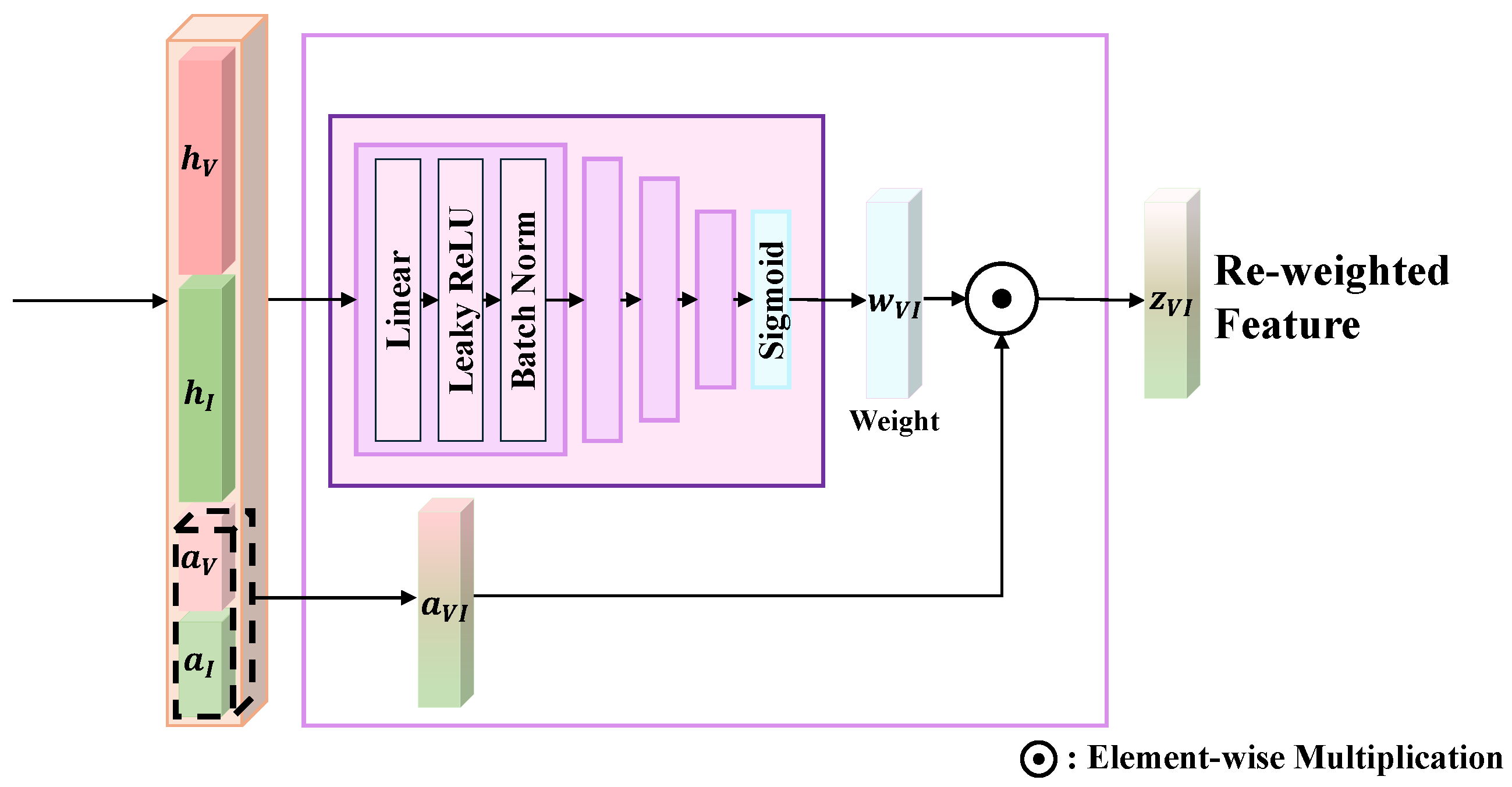
In this section, we propose a fusion module designed to ensure robust pose estimation, even under challenging conditions, such as missing or degraded data. Figure 6 shows the proposed dynamic fusion module architecture. In Figure 6, each sensor’s feature representation carries unique strengths; however, treating all features as equally reliable can lead to significant drift and errors due to environmental changes, sensor instability, or data loss. To mitigate this, the fusion module evaluates the reliability of each sensor’s data and dynamically adjusts the weights assigned to each feature accordingly.

Figure 6. Dynamic Fusion Module Architecture for Sensor Reliability Assessment.

At the core of the fusion module is a dynamic weighting mechanism driven by hidden latent vectors produced by the auxiliary pose estimator. This estimator independently processes each sensor’s features, generating latent vectors that encode its processing experience. These vectors serve as crucial inputs for weight determination, enabling precise fusion that reflects the real-time reliability of each sensor’s features.

The weight determination is implemented via an MLP that takes as input the concatenated visual and inertial feature vectors alongside their corresponding hidden latent vectors from the auxiliary pose estimator. This combined input passes through multiple layers with Leaky ReLU activations and batch normalization to promote stable learning and capture data uncertainties.

The MLP’s architecture begins with a 1024-neuron layer, followed by layers with 512, 256, and 128 neurons, ensuring efficient information flow. The final layer applies a sigmoid activation function to output weight vectors $w_V$ and $w_I$, constrained to the range $[0,1]$. This process is expressed as:

$$\begin{array}{c}\hfill [w_V,w_I]=\mathrm{Sigmoid}\left(\mathrm{MLP}\left([a_V,a_I,h_V,h_I]\right)\right)\end{array}$$

(7)

where $[a_V,a_I,h_V,h_I]$ denotes the concatenation of visual and inertial features $a_V$, $a_I$ with their respective hidden latent vectors $h_V$, $h_I$ from the auxiliary pose estimator. The resulting weights $w_V$ and $w_I$ represent the dynamically assigned reliabilities of the visual and inertial sensor features during fusion.

The fusion module improves localization stability through close interaction with the auxiliary pose estimator. The hidden latent vectors generated by the auxiliary pose estimator encapsulate prior processing experience with each sensor’s features at the current time step, serving as a crucial reference for the fusion module’s assessment of the reliability of incoming data. By dynamically adjusting the weights assigned to each sensor’s data based on this reliability assessment, the fusion module ensures stable and accurate localization performance, even in adverse conditions such as sensor noise or missing data.

Fusion Function

To integrate the high-level features extracted by the visual and inertial encoders, we employ a fusion function g that combines these features into a single unified representation z for downstream pose estimation tasks.

This process is defined as:

$$\begin{array}{c}\hfill z=g(a_V,a_I)\end{array}$$

(8)

The fusion function g merges the visual feature vector $a_V$ and inertial feature vector $a_I$ into a comprehensive representation that captures both spatial and motion-related information. To ensure stable estimation, we explicitly model a feature re-weighting mechanism that accounts for environmental dynamics and sensor reliability. This dynamic re-weighting enables the system to adjust each sensor’s contribution based on the quality and reliability of the incoming data.

Our fusion strategy leverages not only the fused visual-inertial features but also a hidden latent vector generated by an auxiliary pose estimator. This latent vector captures prior temporal context at the same time step and informs the dynamic re-weighting, allowing the model to better reflect real-time changes in sensor reliability.

2.2.4. Learning Methods

Stage-Wise Training

The fusion module dynamically adjusts the weights assigned to each sensor’s data based on its assessed reliability, which is derived from the hidden latent vector generated by the auxiliary pose estimator. This hidden latent vector encapsulates prior experience from processing each sensor’s features, enabling the system to evaluate the quality of incoming sensor data. However, during early training stages, when the auxiliary pose estimator is not yet well-trained, the hidden latent vector may lack reliability or accuracy. Consequently, the fusion module might misjudge sensor reliability, leading to degraded localization accuracy.

To address this issue, we implement a stage-wise training strategy that allows the auxiliary pose estimator to reach a sufficient level of accuracy before enabling dynamic weight adjustments within the fusion module. Figure 7 shows the proposed stage-wise training strategy. This phased approach ensures the model can reliably evaluate sensor data quality, resulting in more stable and robust localization performance. The training process consists of two stages:

Figure 7. Stage-wise Training Strategy for Robust Sensor Data Fusion.

In the first stage, the fusion module is excluded from training. Instead, the feature vectors from each sensor are concatenated directly—without reliability weighting—and passed to the main pose estimator for localization. During this phase, only the weights of the feature encoder, auxiliary pose estimator, and main pose estimator are updated, while the fusion module is omitted. This setup enables the auxiliary pose estimator to learn to generate reliable hidden latent vectors from individual sensor features. The training objective for this stage is expressed as:

$$\begin{array}{c}\hfill \underset{{\theta }_{\mathrm{enc}},{\theta }_{\mathrm{sub}},{\theta }_{\mathrm{main}}}{min}L(y,\widehat{y}({\theta }_{\mathrm{enc}},{\theta }_{\mathrm{sub}},{\theta }_{\mathrm{main}}))\end{array}$$

(9)

where ${\theta }_{\mathrm{enc}}$, ${\theta }_{\mathrm{sub}}$, and ${\theta }_{\mathrm{main}}$ represent the weights of the feature encoder, auxiliary pose estimator, and main pose estimator, respectively.

In the second stage, the fusion module is reintroduced with parameters initialized from the first stage. At this point, the weights of the feature encoder and auxiliary pose estimator are frozen, and only the weights of the fusion module and main pose estimator are updated. This allows the fusion module to dynamically assess sensor reliability, while the main pose estimator continues optimizing localization accuracy. This stage is formulated as:

$$\begin{array}{c}\hfill \underset{{\theta }_{\mathrm{fuse}},{\theta }_{\mathrm{main}}}{min}L(y,\widehat{y}({\theta }_{\mathrm{enc}},{\theta }_{\mathrm{sub}},{\theta }_{\mathrm{main}},{\theta }_{\mathrm{fuse}}))\end{array}$$

(10)

where ${\theta }_{\mathrm{fuse}}$ denotes the weights of the fusion module, ${\theta }_{\mathrm{main}}$ denotes the main pose estimator’s weights, and ${\theta }_{\mathrm{enc}}$ and ${\theta }_{\mathrm{sub}}$ remain fixed from the first stage.

By employing this stage-wise training approach, the auxiliary pose estimator gains the capability to produce sufficiently accurate hidden latent vectors, enabling the fusion module to effectively evaluate the reliability of each sensor feature. This process ultimately improves the overall localization performance.

Loss Function

The proposed robust VIO model takes sequential monocular images and IMU data as inputs, extracting visual and inertial features that are then fused to predict the final pose. The model outputs a 3D translation vector $\mathbf{p}$ and a 3D rotation vector $\mathbf{r}$, where the rotation is represented using Euler angles. During training, the model minimizes the mean squared error (MSE) between the predicted and ground truth poses, encouraging accurate pose estimation. This loss function also guides both the main and auxiliary pose estimators in learning reliable hidden latent vectors that reflect each sensor’s confidence.

To improve pose accuracy, we define an MSE loss that minimizes the difference between predicted and actual poses. This loss is applied to the main pose estimator and each auxiliary pose estimator, ensuring precise localization across varying conditions. The optimal parameters $\theta$ are obtained by minimizing the following pose estimation loss:

$$\begin{array}{c}\hfill L_{\mathrm{pose}}\left(\theta \right)=\parallel \mathbf{p}-\widehat{\mathbf{p}}{\parallel }^2+\lambda {\parallel \mathbf{r}-\widehat{\mathbf{r}}\parallel }^2\end{array}$$

(11)

where $\mathbf{p}$ and $\mathbf{r}$ represent the ground truth relative poses, $\widehat{\mathbf{p}}$ and $\widehat{\mathbf{r}}$ are their predicted values, and $\lambda =100$ is a scaling factor balancing translation and rotation errors, which helps the model maintain accuracy in both domains.

The loss function assigns different weights to the pose losses from the main and auxiliary pose estimators to reflect their relative importance. The main pose estimator, which fuses all sensor data to produce the final pose, is critical for localization performance and is therefore assigned a higher weight $\alpha$ to prioritize its accuracy.

The auxiliary pose estimators, which independently process each sensor’s features to generate hidden latent vectors evaluating sensor data quality, receive a lower weight $\beta =0.5$ to balance training. This weighting accounts for the fact that the main pose estimator—processing fused data—typically converges faster, while auxiliary pose estimators—handling individual sensor inputs—converge more slowly. Properly adjusting $\alpha$ and $\beta$ harmonizes the learning rates and accuracy between these components.

The overall loss function, designed to optimize performance under diverse conditions, is defined as:

$$\begin{array}{c}\hfill L_{\mathrm{total}}=\alpha L_{\mathrm{pose}}^{\mathrm{main}}+\beta L_{\mathrm{pose}}^{\mathrm{sub}\_\mathrm{visual}}+\beta L_{\mathrm{pose}}^{\mathrm{sub}\_\mathrm{inertial}}\end{array}$$

(12)

where $L_{\mathrm{pose}}^{\mathrm{main}}$, $L_{\mathrm{pose}}^{\mathrm{sub}\_\mathrm{visual}}$, and $L_{\mathrm{pose}}^{\mathrm{sub}\_\mathrm{inertial}}$ denote the pose losses of the main pose estimator, visual auxiliary pose estimator, and inertial auxiliary pose estimator, respectively.

This combined loss function enables the model to assess sensor data reliability effectively, thereby improving localization accuracy even in challenging scenarios such as noisy inputs or data dropout. By optimizing this joint loss, the model balances precise localization with robust sensor reliability evaluation.

3. Experimental Results

In this chapter, we present a series of experiments to validate the performance of the proposed robust vehicle pose estimation algorithm. We first evaluate the model’s effectiveness by comparing its results with state-of-the-art deep learning-based methods on the KITTI Odometry dataset [41]. Next, we test the robustness of each model by simulating data-missing scenarios in the KITTI Odometry dataset. Finally, we examine the interpretability of the proposed algorithm by visually analyzing the fusion module and its learned weighting behavior, offering insights into the model’s decision-making process.

3.1. Experimental Setups

3.1.1. Implementation Details

Our framework employs the FlowNetSimple model [42] as the feature encoder, initialized with pretrained weights from the FlyingChairs dataset. This model was originally trained with a learning rate of $1\times {10}^{-3}$, a batch size of 32, and for a total of 695 epochs.

All experiments were conducted using PyTorch (version 1.12.1) on an NVIDIA Quadro RTX 8000 GPU. To ensure a fair comparison, all models were trained under identical experimental conditions. Specifically, we used the Adam optimizer with a batch size of 32. The learning rate and weight decay were adjusted across three training phases: $5\times {10}^{-4}$ for the first 40 epochs, $5\times {10}^{-5}$ for the next 40 epochs, and $1\times {10}^{-6}$ for the final 20 epochs. All models were trained for 100 epochs using input sequences of length 11. Input image resolution was fixed at $256\times 512$ to maintain consistency across experiments.

For the loss function, we set the weights as follows: $\alpha =1$, $\beta =0.5$, and $\lambda =100$ to achieve a balanced optimization between translational and rotational errors and between main and auxiliary estimators.

3.1.2. Comparison Algorithms

To evaluate the effectiveness of our approach, we selected four VIO algorithms for comparison: VINet [43], Soft VIO, Hard VIO [44], and Visual-Selective VIO [45]. VINet uses a simple concatenation-based fusion strategy and serves as a comparison algorithm against more advanced adaptive fusion techniques. The other three algorithms—Soft VIO, Hard VIO, and Visual-Selective VIO—represent state-of-the-art approaches that utilize various adaptive fusion strategies to handle sensor data.

The defining characteristics of each camparison algorithm are summarized below:

• VINet concatenates features from different sensors without evaluating their reliability and uses the combined features for state estimation.
• Soft VIO uses an MLP followed by a sigmoid activation to assign continuous weights in the range $[0,1]$ to each sensor feature before state estimation.
• Hard VIO adopts the Gumbel-Softmax trick to assign discrete weights, giving a weight of 1 to high-quality features and 0 to low-quality ones.
• Visual-Selective VIO relies primarily on inertial features for state estimation, temporarily incorporating visual features only to correct accumulated inertial drift.

This diverse set of comparison algorithms enables a comprehensive evaluation of performance across various sensor fusion strategies.

3.1.3. Dataset

KITTI Odometry Dataset

The KITTI Odometry dataset consists of 11 sequences (00–10) containing visual images, IMU measurements, GPS data, and ground truth. It is widely used as a benchmark for localization tasks such as odometry and SLAM. In this study, we use this dataset to estimate both vehicle position and orientation by fusing visual, inertial, and GPS data.

For training our deep neural network model, we used sequences 00, 01, 02, 04, 06, 08, and 09. Sequence 03 was excluded due to missing data files. Sequences 07 and 10, which are relatively long, were reserved for evaluation.

The KITTI Odometry dataset presents several challenges, including a low image frame rate of 10 Hz, high vehicle speeds, dynamic scenes with moving objects, and varying lighting conditions due to shadows from buildings and trees. The dataset provides synchronized image, GPS, and ground truth data at 10 Hz, while IMU measurements are recorded at a higher frequency of 100 Hz. We used the dataset for both training and evaluation.

Synthetic Data Missing

To assess the model’s robustness under sensor data loss, we created a synthetic dataset by introducing missing data scenarios based on the KITTI Odometry dataset. Data dropout was simulated across three sensor modalities: camera, IMU, and GPS, each with 30% missing data.

We designed both deterministic and stochastic patterns of data loss. In deterministic scenarios, data was removed from continuous intervals, simulating conditions like passing through tunnels or underpasses. These intervals were set to achieve 30% total data loss for each modality. In stochastic scenarios, data points were randomly dropped using a Bernoulli process, again ensuring 30% data loss per modality across the dataset.

These synthetic data-missing conditions reflect realistic challenges such as sensor disconnections, packet loss, excessive load, and environmental interference. They allow for a thorough evaluation of the model’s robustness in the presence of unreliable or incomplete sensor inputs.

3.1.4. Evaluation Metrics

To evaluate the performance of the proposed algorithm, we computed the root mean squared error (RMSE) between the predicted outputs and the ground truth values for both position and orientation. The metrics are separated into position errors for the x and y coordinates, and orientation errors for the yaw angle $\theta$.

Position Error RMSE

The RMSE for each positional axis x and y is calculated as follows:

$$\begin{array}{c}\hfill {\mathrm{RMSE}}_x=\sqrt{{\displaystyle \frac{1}{N}}\sum _{i=1}^N{(x_i-{\widehat{x}}_i)}^2}\end{array}$$

(13)

$$\begin{array}{c}\hfill {\mathrm{RMSE}}_y=\sqrt{{\displaystyle \frac{1}{N}}\sum _{i=1}^N{(y_i-{\widehat{y}}_i)}^2}\end{array}$$

(14)

where $x_i$ and $y_i$ are the ground truth positions at time step i, and ${\widehat{x}}_i$ and ${\widehat{y}}_i$ are the corresponding predicted positions. N represents the total number of time steps.

Orientation Error RMSE

The RMSE for the orientation angle $\theta$ is given by:

$$\begin{array}{c}\hfill {\mathrm{RMSE}}_{\theta }=\sqrt{{\displaystyle \frac{1}{N}}\sum _{i=1}^N{({\theta }_i-{\widehat{\theta }}_i)}^2}\end{array}$$

(15)

where ${\theta }_i$ and ${\widehat{\theta }}_i$ represent the ground truth and predicted orientation angles at each time step, respectively.

3.1.5. Total Position Errors

To quantify the model’s overall positional accuracy, we define a combined metric called total position error, calculated as the L2 norm of the positional RMSE values in the x and y directions:

$$\begin{array}{c}\hfill {\mathrm{RMSE}}_{\mathrm{position}}=\sqrt{{\mathrm{RMSE}}_x^2+{\mathrm{RMSE}}_y^2}\end{array}$$

(16)

This comprehensive RMSE-based evaluation framework provides a reliable measure of the model’s performance in terms of localization accuracy across various operational conditions, including scenarios with missing sensor data.

3.2. Comparison with VIO Methods

3.2.1. Quantitative and Qualitative Results

This section presents a detailed comparison of the proposed algorithm against four state-of-the-art VIO methods: Visual-Selective VIO, Hard VIO, Soft VIO, and VINet. The evaluation covers five scenarios: Normal, GPS Deterministic Missing, GPS Stochastic Missing, GPS Deterministic and Visual Missing, and GPS Stochastic and Visual Missing. Experiments were conducted on Sequences 07 and 10 from the KITTI odometry dataset to maintain evaluation consistency. The normal scenario represents standard conditions with no missing data, serving as a comparison algorithm. The GPS Deterministic Missing scenario simulates continuous absence of GPS data over specific intervals, while the GPS Stochastic Missing scenario assumes approximately 30% random GPS data dropout.

The GPS Deterministic and Visual Missing scenario combines deterministic GPS data loss with stochastic visual data dropout affecting approximately 30% of the visual inputs. Likewise, the GPS Stochastic and Visual Missing scenario assumes roughly 30% random loss of both GPS and visual data. For each scenario, RMSE was computed independently for positional and orientation errors. To complement this quantitative analysis, qualitative trajectory comparisons were also performed to provide deeper insight into each algorithm’s behavior under various missing data conditions.

Table 1 summarizes the position and orientation RMSEs of each algorithm across all scenarios and sequences. In this table, the lowest RMSE in each scenario is highlighted in bold, while the second-lowest is underlined. In the normal scenario, the proposed algorithm achieved the lowest position RMSE, with values of 2.07 m for sequence 07 and 8.63 m for sequence 10. For orientation RMSE, Visual-Selective VIO slightly outperformed others on sequence 10, recording 4.26°, with the proposed method ranking second at 9.10°. In the GPS Deterministic Missing scenario, despite the complete absence of GPS data, the proposed algorithm maintained superior performance, achieving position RMSEs of 3.61 m and 11.76 m for sequences 07 and 10, respectively.

Table 1. Comparison of Position and Orientation RMSE Across Different Scenarios and Sequences GD-V Missing: GPS Deterministic and Visual Missing GS-V Missing: GPS Stochastic and Visual Missing.

Scenario	Error (RMSE)	Ours		VS VIO [45]		Hard VIO [44]		Soft VIO [44]		VINet [43]
Sequence		7	10	7	10	7	10	7	10	7	10
Normal	Position (m)	2.07	8.63	6.34	16.77	11.96	129.18	10.46	121.88	10.85	122.1
	Orientation (°)	9.43	9.10	4.64	4.26	2.70	27.78	2.51	23.32	2.41	23.52
GD Missing	Position (m)	3.61	11.76	6.34	16.77	11.96	129.18	10.46	121.88	10.85	122.1
	Orientation (°)	9.43	9.10	4.64	4.26	2.70	27.78	2.51	23.32	2.41	23.52
GS Missing	Position (m)	1.64	8.62	6.34	16.77	11.96	129.18	10.46	121.88	10.85	122.1
	Orientation (°)	9.43	9.10	4.64	4.26	2.70	27.78	2.51	23.32	2.41	23.52
GD-V Missing	Position (m)	4.11	13.14	26.17	63.23	27.05	33.21	27.77	36.58	36.46	78.88
	Orientation (°)	10.11	2.13	4.48	7.38	15.01	2.57	15.03	5.57	24.58	16.09
GS-V Missing	Position (m)	1.66	8.65	26.17	63.23	27.05	33.21	27.77	36.58	36.46	78.88
	Orientation (°)	10.11	2.13	4.48	7.38	15.01	2.57	15.03	5.57	24.58	16.09

Under the GPS Stochastic Missing scenario—where roughly 30% of GPS data was randomly lost—the proposed method preserved performance comparable to the normal scenario, demonstrating strong tolerance to stochastic GPS dropout. In the GPS Deterministic and Visual Missing scenario, the proposed algorithm recorded the lowest position RMSEs for both Sequences 07 and 10 maintained strong orientation accuracy. Similarly, in the GPS Stochastic and Visual Missing scenario, it consistently achieved the best results across sequences and metrics, illustrating exceptional resilience to simultaneous GPS and visual data loss. Overall, these results underscore the reliability of the proposed algorithm across diverse data missing conditions, highlighting its potential for practical deployment in challenging real-world environments.

Although the proposed method achieves competitive orientation accuracy, it does not consistently outperform all baselines. This limitation results from the absence of global heading cues. Without GPS-based orientation information, the VIO module tends to overfit to position loss during training, which may compromise orientation accuracy.

To ensure fair comparison with standard SLAM/VIO benchmarks, we additionally report the $t_{\mathrm{rel}}$ and $r_{\mathrm{rel}}$ metrics. As shown in Table 2, these results are consistent with the RMSE-based evaluations.

Table 2. Comparison of Translational and Rotational Errors Across Different Scenarios and Sequences GD-V Missing: GPS Deterministic and Visual Missing GS-V Missing: GPS Stochastic and Visual Missing $t_{\mathrm{rel}}$ and $r_{\mathrm{rel}}$ are the average translational error (%) and average rotational error (°/100 m) obtained from various segment lengths of 100–800 m.

Scenario	Error	Ours		VS VIO [45]		Hard VIO [44]		Soft VIO [44]		VINet [43]
Sequence		7	10	7	10	7	10	7	10	7	10
Normal	$t_{\mathrm{rel}}$ (%)	1.44	3.23	2.87	5.24	4.87	15.20	4.46	14.84	4.52	14.85
	$r_{\mathrm{rel}}$ (°)	2.46	2.42	1.64	1.57	1.21	4.51	1.14	4.16	1.09	4.18
GD Missing	$t_{\mathrm{rel}}$ (%)	2.09	4.81	2.87	5.24	4.87	15.20	4.46	14.84	4.52	14.85
	$r_{\mathrm{rel}}$ (°)	2.46	2.42	1.64	1.57	1.21	4.51	1.14	4.16	1.09	4.18
GS Missing	$t_{\mathrm{rel}}$ (%)	1.28	3.23	2.87	5.24	4.87	15.20	4.46	14.84	4.52	14.85
	$r_{\mathrm{rel}}$ (°)	2.46	2.42	1.64	1.57	1.21	4.51	1.14	4.16	1.09	4.18
GD-V Missing	$t_{\mathrm{rel}}$ (%)	2.23	5.02	7.43	10.75	7.52	8.14	7.60	8.45	8.44	11.77
	$r_{\mathrm{rel}}$ (°)	2.64	0.97	1.62	2.15	3.30	1.15	3.30	1.84	4.27	3.46
GS-V Missing	$t_{\mathrm{rel}}$ (%)	1.29	3.24	7.43	10.75	7.52	8.14	7.60	8.45	8.44	11.77
	$r_{\mathrm{rel}}$ (°)	2.64	0.97	1.62	2.15	3.30	1.15	3.30	1.84	4.27	3.46

Table 3 presents the RMSE values for the x and y positional axes and the $\theta$ orientation angle in the Normal scenario for sequence 07. The proposed algorithm achieved the lowest RMSE values, with 1.20 m for the x axis and 1.69 m for the y axis, demonstrating high precision in position estimation. Similarly, Table 4 shows the results for sequence 10, where the proposed algorithm again delivered superior performance, recording the lowest RMSEs of 7.37 m and 4.49 m for the x and y axes, respectively.

Table 3. Detailed RMSE for x, y Position and $\theta$ Orientation in Normal Scenario (Sequence 07).

Error (RMSE)	Ours	VS VIO	Hard VIO	Soft VIO	VINet
x (m)	1.20	4.26	6.84	7.95	6.10
y (m)	1.69	4.69	9.81	6.80	8.97
$\theta$ (°)	9.43	4.64	2.70	2.51	2.41

Table 4. Detailed RMSE for x, y Position and $\theta$ Orientation in Normal Scenario (Sequence 10).

Error (RMSE)	Ours	VS VIO	Hard VIO	Soft VIO	VINet
x (m)	7.37	11.62	32.24	26.58	26.88
y (m)	4.49	12.09	125.09	118.95	119.10
$\theta$ (°)	9.10	4.26	27.78	23.32	23.52

Figure 8 presents trajectory visualizations that support these quantitative results. As shown in Figure 8, proposed method follows the ground truth trajectory more closely and accurately than the competing algorithms. The strong alignment between numerical metrics and trajectory comparisons underscores the consistency and accuracy of the proposed approach under standard conditions. Collectively, these findings validate its effectiveness for precise localization tasks.

Figure 8. Trajectory Comparison in Normal Scenario. Yellow boxes indicate turning segments where baselines drift, while the proposed method maintains trajectory accuracy with GPS correction.

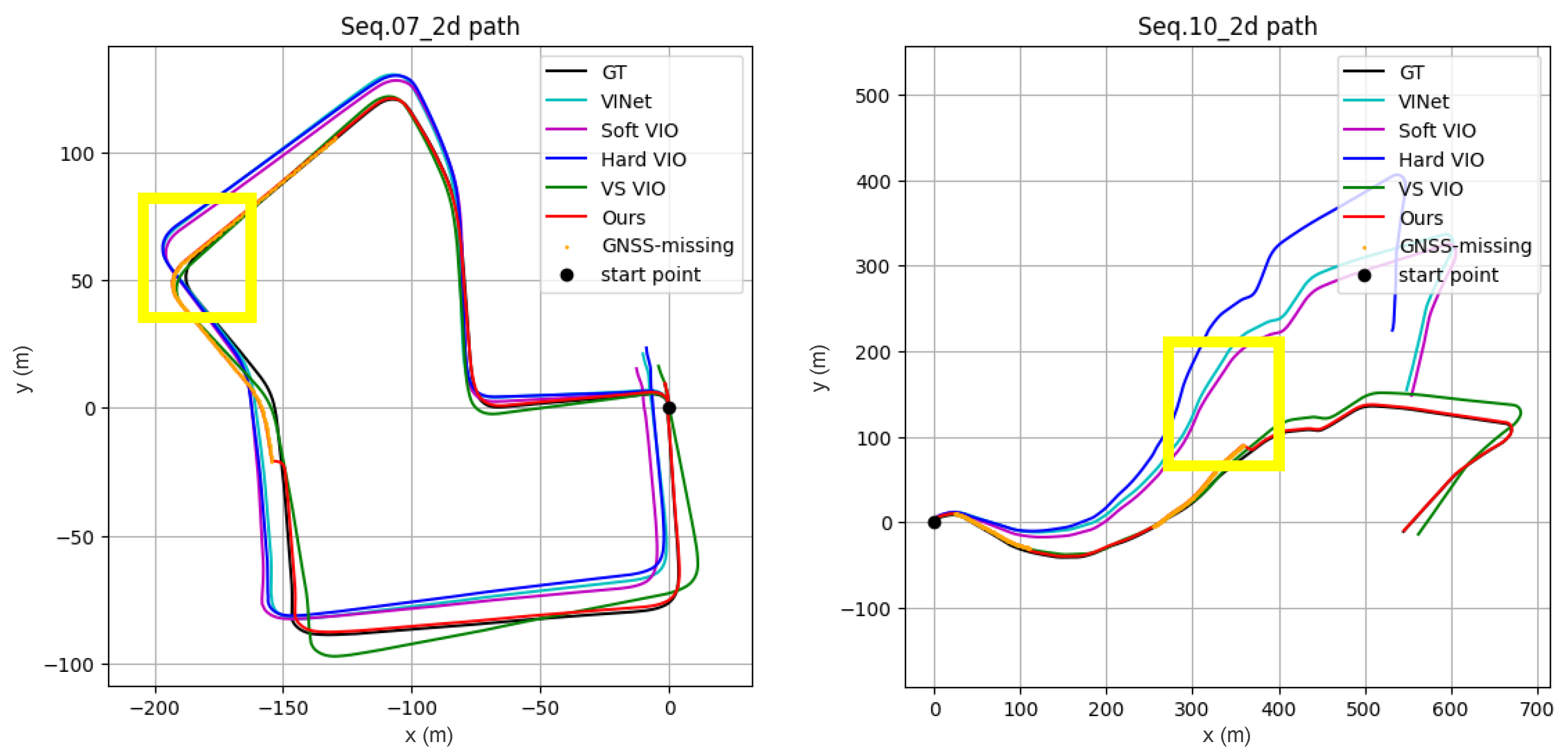
Table 5 and Table 6 summarize the RMSE results for Sequences 07 and 10 in the GPS deterministic missing scenario. For Sequence 07, the proposed algorithm exhibited outstanding performance, achieving the lowest RMSE of 2.41 m along the y-axis, surpassing all other methods in accuracy. In sequence 10, the proposed method attained the best results across both positional axes (x and y), further confirming its tolerance to GPS data loss. These results emphasize the model’s capability to maintain precise localization even under challenging conditions where critical GPS data is unavailable. Figure 9 provides trajectory comparisons that visually confirm the algorithm’s superior performance, showing its close adherence to the ground truth path. The figure also marks GPS missing intervals with orange scatter points, clearly illustrating data dropout periods and highlighting the method’s consistent accuracy throughout these gaps. This integration of quantitative RMSE data with qualitative trajectory insights confirms the proposed method’s reliability under various GPS missing data scenarios.

Table 5. RMSE Results for GPS Deterministic Missing Scenario (Sequence 07).

Error (RMSE)	Ours	VS VIO	Hard VIO	Soft VIO	VINet
x (m)	2.69	4.26	6.84	7.95	6.10
y (m)	2.41	4.69	9.81	6.80	8.97
$\theta$ (°)	9.43	4.64	2.70	2.51	2.41

Table 6. RMSE Results for GPS Deterministic Missing Scenario (Sequence 10).

Error (RMSE)	Ours	VS VIO	Hard VIO	Soft VIO	VINet
x (m)	9.27	11.62	32.24	26.58	26.88
y (m)	7.24	12.09	125.09	118.95	119.10
$\theta$ (°)	9.10	4.26	27.78	23.32	23.52

Figure 9. Trajectory Comparison for GPS Deterministic Missing Scenario. Yellow boxes indicate turning segments under deterministic GPS loss, where drift accumulates for both baselines and the proposed method due to missing corrections.

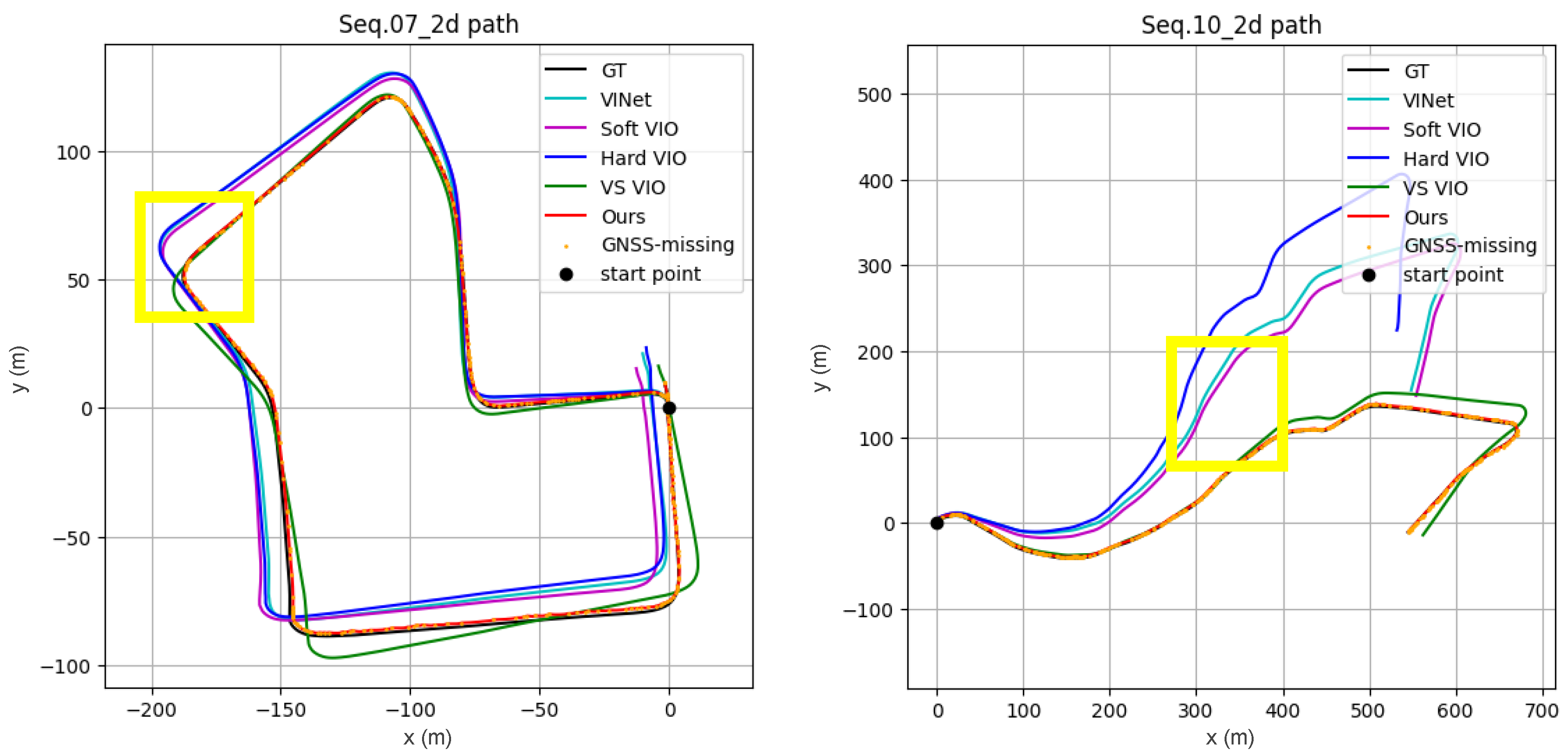
In the GPS Stochastic Missing scenario, the proposed algorithm maintained performance nearly identical to that in the Normal scenario, despite the random loss of GPS data. Table 7 and Table 8 present the results for sequences 07 and 10, respectively, showing that the proposed method consistently achieved the lowest RMSE values among all compared algorithms. These results highlight the algorithm’s ability to preserve localization accuracy even under unpredictable GPS data loss. Additionally, trajectory comparisons shown in Figure 10 visually confirm the proposed algorithm’s ability to closely track the ground truth trajectories, despite the stochastic nature of the missing GPS data. In these figures, GPS missing intervals are marked with orange scatter points, clearly illustrating the data loss regions and the algorithm’s continued accuracy throughout these periods. These findings reinforce the reliability and effectiveness of the proposed approach in handling random GPS data loss, ensuring stable localization performance in real-world scenarios.

Table 7. RMSE Results for GPS Stochastic Missing Scenario (Sequence 07).

Error (RMSE)	Ours	VS VIO	Hard VIO	Soft VIO	VINet
x (m)	1.20	4.26	6.84	7.95	6.10
y (m)	1.11	4.69	9.81	6.80	8.97
$\theta$ (°)	9.43	4.64	2.70	2.51	2.41

Table 8. RMSE Results for GPS Stochastic Missing Scenario (Sequence 10).

Error (RMSE)	Ours	VS VIO	Hard VIO	Soft VIO	VINet
x (m)	7.31	11.62	32.24	26.58	26.88
y (m)	4.56	12.09	125.09	118.95	119.10
$\theta$ (°)	9.10	4.26	27.78	23.32	23.52

Figure 10. Trajectory Comparison for GPS Stochastic Missing Scenario. Trajectory comparison under GPS stochastic dropout. Yellow boxes indicate turning segments under stochastic GPS loss. The proposed method suppresses drift through Kalman filter updates, unlike the baselines.

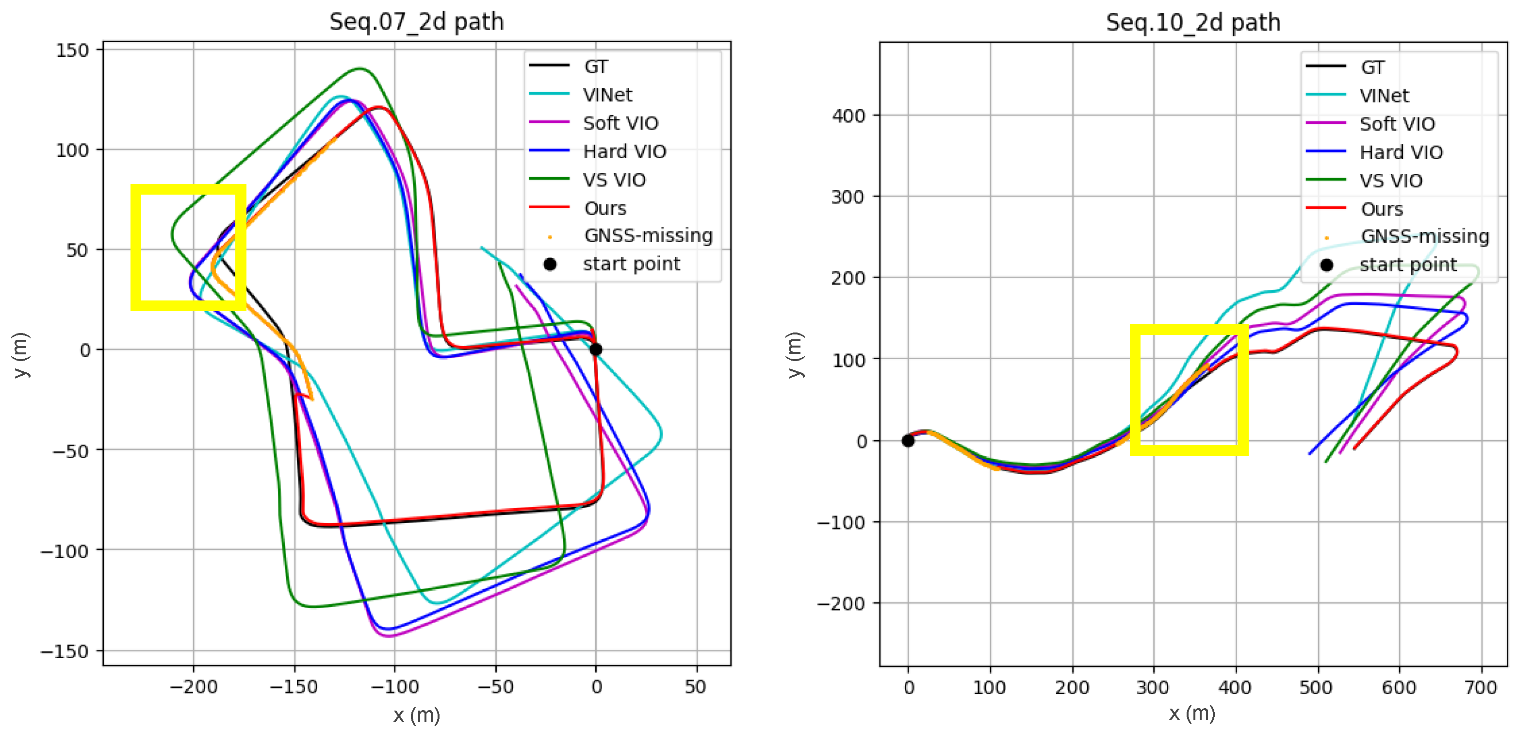
Table 9 and Table 10 present the results for the scenario that represents the most challenging condition, where both GPS and visual data are simultaneously missing. Despite these severe constraints, the proposed algorithm maintained consistent performance, achieving the lowest RMSE values of 1.99 m (x-axis), 3.60 m (y-axis), and 10.11° ($\theta$) for Sequence 07. In Sequence 10, the algorithm continued to outperform all competing methods across the position axes, further demonstrating its adaptability to complex data loss scenarios. Trajectory comparisons in Figure 11 provide additional validation, clearly illustrating the algorithm’s ability to closely follow the ground truth trajectories, even when both GPS and visual data are intermittently unavailable. These comprehensive results underscore the proposed method’s effectiveness and reliability in maintaining accurate localization under the most adverse and realistic data-missing conditions.

Table 9. RMSE Results for GPS Deterministic Missing and Visual Missing Scenario (Sequence 07).

Error (RMSE)	Ours	VS VIO	Hard VIO	Soft VIO	VINet
x (m)	1.99	17.22	19.11	18.92	30.29
y (m)	3.60	19.71	19.15	20.32	20.29
$\theta$ (°)	10.11	4.48	15.01	15.03	24.58

Table 10. RMSE Results for GPS Deterministic Missing and Visual Missing Scenario (Sequence 10).

Error (RMSE)	Ours	VS VIO	Hard VIO	Soft VIO	VINet
x (m)	10.04	25.91	21.00	13.70	12.10
y (m)	8.48	57.68	25.73	33.92	77.95
$\theta$ (°)	2.13	7.38	2.57	5.57	16.09

Figure 11. Trajectory Comparison for GPS Deterministic Missing and Visual Missing Scenario. Yellow boxes indicate turning segments under deterministic GPS loss, where drift accumulates for both baselines and the proposed method due to missing corrections.

In this challenging scenario, the proposed algorithm consistently achieved the lowest RMSE values across both sequences, remaining effective when GPS and visual data are simultaneously unavailable.

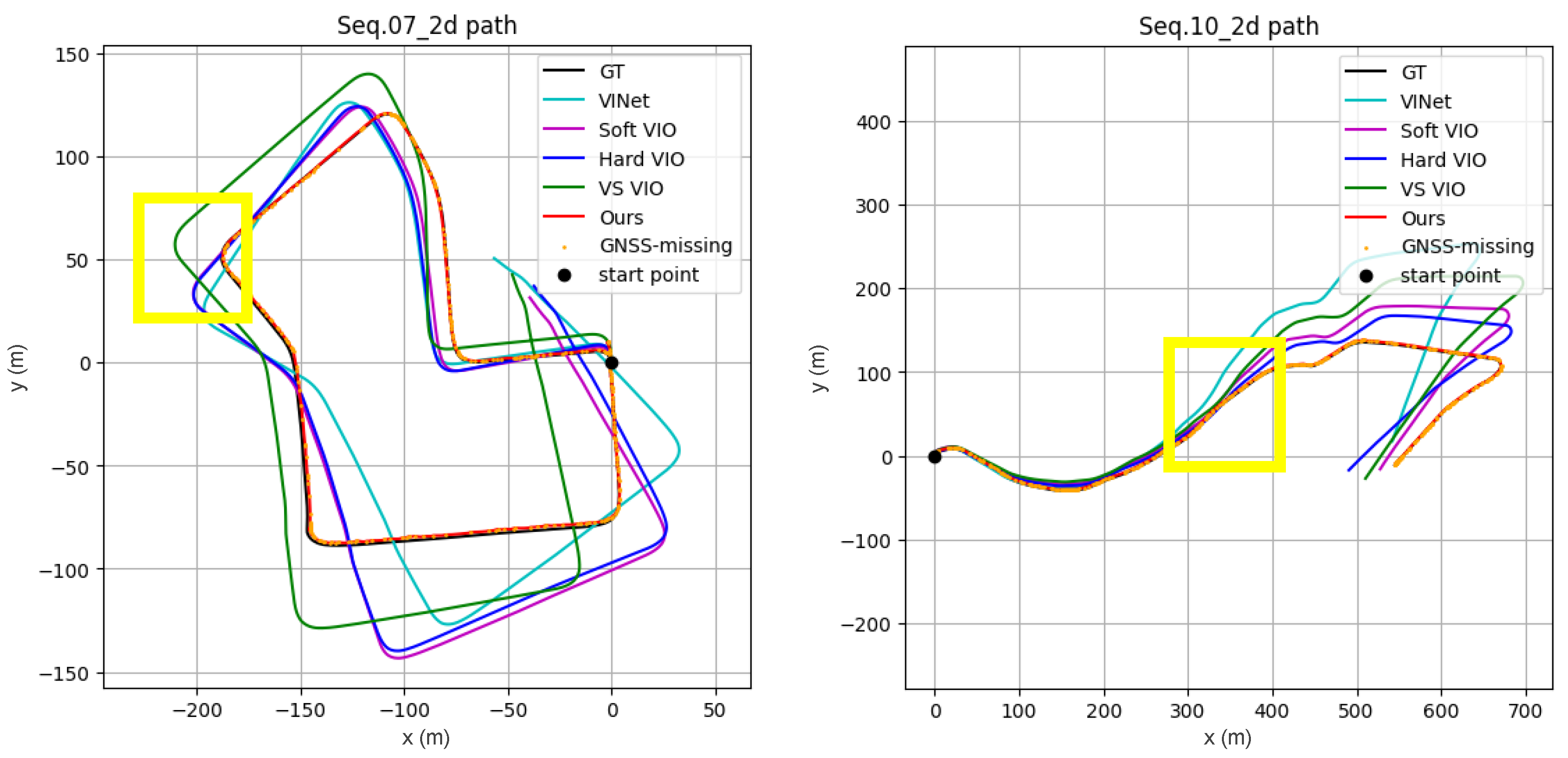
Table 11 and Table 12 present the detailed results for sequences 07 and 10, respectively, highlighting the superior accuracy of the proposed method compared to other algorithms. The trajectory comparisons shown in Figure 12 further validate this performance, clearly illustrating the algorithm’s ability to closely follow the ground truth trajectories despite significant data loss. These visual results emphasize the method’s reliability under conditions where both GPS and visual data are intermittently unavailable. Overall, the findings confirm the proposed algorithm’s strong potential for real-world applications, particularly in environments that demand robust localization under adverse and uncertain data conditions.

Table 11. RMSE Results for GPS Stochastic Missing and Visual Missing Scenario (Sequence 07).

Error (RMSE)	Ours	VS VIO	Hard VIO	Soft VIO	VINet
x (m)	1.23	17.22	19.11	18.92	30.29
y (m)	1.11	19.71	19.15	20.32	20.29
$\theta$ (°)	10.11	4.48	15.01	15.03	24.58

Table 12. RMSE Results for GPS Stochastic Missing and Visual Missing Scenario (Sequence 10).

Error (RMSE)	Ours	VS VIO	Hard VIO	Soft VIO	VINet
x (m)	7.39	25.91	21.00	13.70	12.10
y (m)	4.49	57.68	25.73	33.92	77.95
$\theta$ (°)	2.13	7.38	2.57	5.57	16.09

Figure 12. Trajectory Comparison for GPS Stochastic Missing and Visual Missing Scenario. Trajectory comparison under GPS stochastic dropout. Yellow boxes indicate turning segments under stochastic GPS loss. The proposed method suppresses drift through Kalman filter updates, unlike the baselines.

3.2.2. Real-Time Performance and Resource Consumption

To assess the real-time capability of our approach, we evaluated the time required to process a single frame and calculated the corresponding frames per second (FPS). All experiments were conducted on an NVIDIA Quadro RTX 8000 GPU to ensure consistent and reliable benchmarking. The reported processing time represents an average over 2761 trials. As shown in Table 13, our method achieves an average processing time of 0.0346 s per frame, equivalent to 29 FPS. These results confirm that our approach meets the requirements for real-time processing, making it highly suitable for deployment in practical, time-sensitive applications.

Table 13. Comparative Analysis of Real-Time Capability and System Resource Usage.

Method	Processing Time (s)	FPS	CPU Mem (MB)	GPU Alloc. (MB)	GPU Reserv. (MB)
VINet	0.0250	40	1030.09	464.86	632.00
Soft VIO	0.0262	38	1093.02	466.37	738.00
Hard VIO	0.0278	36	1113.36	469.37	632.00
VS VIO	0.0244	41	1109.98	466.84	632.00
Ours	0.0346	29	1037.61	667.00	774.00

However, although our method achieves 29 FPS on a high-end GPU, it requires relatively higher GPU memory allocation (667 MB) and reservation (774 MB) compared to baselines. This level of resource usage may limit its applicability in embedded deployments. In particular, the auxiliary pose estimation module contributes significantly to the overall computational load and memory footprint.

3.3. Ablation Studies

In this section, we conduct ablation studies to evaluate the contributions of three key components: the auxiliary pose estimator, the fusion module, and the stage-wise learning strategy.

These studies were performed across all scenarios and sequences, and the results are summarized in Table 14.

Table 14. Results of the Ablation Study Demonstrating the Effectiveness of the Proposed Components.

Auxiliary pose estimator				✓				✓		✓
Fusion module						✓		✓		✓
Stage-wise learning										✓
Scenario	Error (RMSE)	7	10	7	10	7	10	7	10	7	10
Normal	Position (m)	2.32	8.81	2.20	8.72	2.20	8.72	2.17	8.68	2.07	8.63
	Orientation (°)	14.21	19.20	10.07	10.61	10.11	10.82	10.00	10.50	9.43	9.10
GD Missing	Position (m)	9.13	13.04	4.37	12.39	4.47	12.48	4.08	12.12	3.61	11.76
	Orientation (°)	14.21	19.20	10.07	10.61	10.11	10.82	10.00	10.50	9.43	9.10
GS Missing	Position (m)	1.84	8.92	1.79	8.81	1.80	8.83	1.75	8.74	1.64	8.62
	Orientation (°)	14.21	19.20	10.07	10.61	10.11	10.82	10.00	10.50	9.43	9.10
GD-V Missing	Position (m)	6.05	15.55	4.31	14.64	3.57	14.35	2.89	13.81	1.68	13.14
	Orientation (°)	14.58	17.82	11.77	10.31	11.62	10.01	11.18	6.01	10.11	2.13
GS-V Missing	Position (m)	1.93	8.92	1.88	8.89	1.83	8.85	1.80	8.83	1.66	8.65
	Orientation (°)	14.58	17.82	11.77	10.31	11.62	10.01	11.18	6.01	10.11	2.13

• Auxiliary Pose Estimator: This component was designed to enhance the assessment of sensor reliability by generating hidden latent vectors. As shown in Table 14, incorporating the auxiliary pose estimator led to noticeable performance gains, particularly in scenarios where sensor data was missing. These results demonstrate its effectiveness in supporting accurate pose estimation under data-deficient conditions.
• Fusion Module: The integration of the fusion module further enhanced performance by dynamically adjusting the weights of sensor features according to their estimated reliability. This adaptive mechanism proved particularly effective in scenarios involving simultaneous sensor data losses—such as GD-V and GS-V missing—where it significantly reduced localization errors by prioritizing more trustworthy inputs.
• Stage-wise Learning: The stage-wise learning strategy improved overall model performance by sequentially optimizing individual components. In this approach, the feature encoders and the primary pose estimator were trained first, followed by the activation of the fusion module. This structured training process facilitated more stable and efficient learning. As shown in Table 14, this incremental refinement yielded consistent performance improvements across all evaluated scenarios and sequences.

3.4. Visualization of Adaptive Weighting Mechanism

In this section, we analyze the dynamic weight adjustment process carried out by the fusion module in the proposed algorithm. Figure 13 and Figure 14 illustrate how the weights assigned to visual and inertial features evolve in response to varying visual data availability. These visualizations offer key insights into the adaptability of our approach and its capability to maintain performance despite data loss. Specifically, Figure 13 presents results for Sequence 07, while Figure 14 corresponds to Sequence 10. Each figure includes two plots: the upper plot shows visual data availability, and the lower plot displays the corresponding weight adjustments for visual and inertial features.

Figure 13. Visualization of Weight Adjustment Process for Sequence 07.

Figure 14. Visualization of Weight Adjustment Process for Sequence 10.

In the upper plot of each figure, the x-axis denotes time in seconds, and the y-axis indicates the presence of visual data. Black lines and dots represent the availability status: a y-value of 1 signifies that visual data is fully available, while a y-value of 0 indicates its complete absence. This binary representation clearly identifies time intervals when visual data is missing. In the lower plot, the x-axis again represents time, while the y-axis indicates weight values ranging from 0 to 1. The red line shows the weight assigned to visual features, and the green line shows the weight assigned to inertial features. Importantly, the sum of these weights always equals 1, reflecting the fusion module’s ability to dynamically balance contributions from the two sensor modalities.

When visual data is fully available (y = 1 in the upper plot), the red and green lines in the lower plot remain steady and approximately parallel, indicating stable and consistent weighting. For instance, in Figure 13, the interval from 89 to 90 s illustrates how the weights for both features remain constant when visual data is consistently accessible. This stability confirms the algorithm’s ability to maintain a reliable sensor balance under normal operating conditions.

In contrast, during intervals of visual data loss (y = 0 in the upper plot), the red line in the lower plot drops, while the green line rises accordingly. This behavior illustrates the fusion module’s capacity to compensate for missing visual information by increasing reliance on inertial data. For example, in Figure 14, between 2 and 4 s, the visual feature weight decreases markedly, while the inertial feature weight increases. Such dynamic adjustment helps the algorithm remain robust even when visual inputs become intermittently unavailable.

Notably, even when visual data is completely absent, the weight assigned to visual features does not drop to zero. Instead, it decreases to a minimal value, ensuring a small but persistent contribution. This design allows the model to exploit any partially available or rapidly fluctuating visual input, thus improving resilience. Such a strategy avoids full dependency on inertial data and makes optimal use of all available sensor information to sustain localization accuracy.

These observations underscore the effectiveness of the fusion module in adaptively regulating sensor contributions based on data availability. By down-weighting unreliable visual features and compensating with inertial data, the module achieves stable performance without over-reliance on a single sensor source. Nonetheless, further research is warranted to determine the optimal threshold for retaining visual feature weights during visual data dropout, with the goal of maximizing both stability and accuracy.

In summary, the visualizations in Figure 13 and Figure 14 demonstrate the algorithm’s ability to adaptively manage sensor contributions in real time. The fusion module ensures reliable localization performance by intelligently reallocating weights between visual and inertial inputs—even under conditions of significant visual data loss. This balanced, data-aware fusion strategy highlights the algorithm’s strong potential for deployment in real-world environments where sensor reliability may vary.

4. Limitations and Future Work

While the proposed algorithm demonstrates reliable performance under various sensor-degraded scenarios, certain limitations remain. A key challenge lies in orientation estimation due to the absence of global heading information. Accurate heading estimation is challenged by the lack of absolute orientation data from GPS, which provides only positional information. Without an external reference for global heading, it becomes fundamentally ambiguous to resolve orientation from the relative motion cues of visual and inertial sensors alone. This limitation may lead the learning process to emphasize positional accuracy over orientation precision. The current implementation adopts Euler-angle representations and empirically balanced loss weights, following standard practice in visual-inertial odometry research. Future work may consider integrating additional global orientation sources or introducing refined regularization strategies to more explicitly balance the position and orientation objectives.

In terms of computational efficiency, the algorithm operates in real time on high-end GPU hardware but requires a relatively large memory footprint. This is primarily due to the auxiliary pose estimation module, which enhances robustness at the cost of increased resource usage. Such requirements may limit applicability in embedded or resource-constrained environments. Potential directions for improvement include model pruning, quantization, and the use of lightweight encoder architectures to facilitate deployment on edge platforms.

5. Conclusions

In this study, we proposed a novel and robust vehicle pose estimation algorithm designed to address the challenges posed by unpredictable environments and unreliable sensor data. By effectively fusing information from visual, inertial, and GPS sensors, the algorithm maintains reliable performance even under both stochastic and deterministic data loss conditions. At the core of the system is the Robust VIO module, which dynamically assesses sensor reliability using a fusion mechanism and captures temporal dependencies via an LSTM-based pose estimator to generate accurate local pose estimates. In parallel, GPS data is evaluated independently by a reliability detector and adaptively fused with VIO outputs through a Kalman filter. This modular architecture allows the system to flexibly adapt to varying sensor conditions and environmental dynamics, ensuring stable and precise localization.

Extensive experiments showed consistent performance of the proposed approach across a wide range of challenging scenarios, including significant GPS and visual data loss. The algorithm consistently achieved the lowest RMSE values compared to state-of-the-art baselines, highlighting its superior performance under both random and structured missing data. Trajectory comparisons further reinforced its capability to closely follow ground truth paths, even in the presence of substantial sensor degradation, affirming its practical value for real-world applications such as autonomous driving and robotic navigation. Moreover, the visualizations of dynamic sensor weight adjustments offered key insights into the system’s adaptability, showcasing its ability to intelligently utilize available data while minimizing the impact of unreliable inputs.

Future work will focus on expanding the algorithm’s applicability to more complex and diverse environments. Emphasis will be placed on enhancing sensor reliability assessment and further optimizing the dynamic weighting mechanism to improve overall localization accuracy and stability. These efforts aim to strengthen the system’s utility as a core component in next-generation navigation frameworks, especially in scenarios where sensor quality is inconsistent or unpredictable.

In summary, this study represents a significant advancement in localization technologies by introducing an adaptive and resilient framework capable of intelligently balancing sensor inputs across diverse and challenging conditions. The methods and findings presented here lay a strong foundation for the continued development of reliable, intelligent, and real-time localization systems applicable to a broad range of domains.

References

1. Kim, K.W.; Im, J.H.; Jee, G.I. Tunnel facility based vehicle localization in highway tunnel using 3D LIDAR. IEEE Trans. Intell. Transp. Syst. 2022, 23, 17575–17583. [Google Scholar] [CrossRef]
2. Wen, T.; Jiang, K.; Wijaya, B.; Li, H.; Yang, M.; Yang, D. TM 3 Loc: Tightly-coupled monocular map matching for high precision vehicle localization. IEEE Trans. Intell. Transp. Syst. 2022, 23, 20268–20281. [Google Scholar] [CrossRef]
3. Moreau, A.; Piasco, N.; Tsishkou, D.; Stanciulescu, B.; de La Fortelle, A. Coordinet: Uncertainty-aware pose regressor for reliable vehicle localization. In Proceedings of the IEEE/CVF Winter Conference on Applications of Computer Vision (WACV), Waikoloa, HI, USA, 3–8 January 2022; pp. 2229–2238. [Google Scholar]
4. Zhou, Z.; Li, L.; Fürsterling, A.; Durocher, H.J.; Mouridsen, J.; Zhang, X. Learning-based object detection and localization for a mobile robot manipulator in SME production. Robot. -Comput.-Integr. Manuf. 2022, 73, 102229. [Google Scholar] [CrossRef]
5. Savci, I.H.; Yilmaz, A.; Karaman, S.; Ocakli, H.; Temeltas, H. Improving navigation stack of a ros-enabled industrial autonomous mobile robot (amr) to be incorporated in a large-scale automotive production. Int. J. Adv. Manuf. Technol. 2022, 120, 3647–3668. [Google Scholar] [CrossRef]
6. Liu, Q.; Cong, Q. Kinematic and dynamic control model of wheeled mobile robot under internet of things and neural network. J. Supercomput. 2022, 78, 8678–8707. [Google Scholar] [CrossRef]
7. Sun, Y.; Wang, W.; Mottola, L.; Zhang, J.; Wang, R.; He, Y. Indoor drone localization and tracking based on acoustic inertial measurement. IEEE Trans. Mob. Comput. 2023, 23, 7537–7551. [Google Scholar] [CrossRef]
8. Zhang, P.; Chen, G.; Li, Y.; Dong, W. Agile formation control of drone flocking enhanced with active vision-based relative localization. IEEE Robot. Autom. Lett. 2022, 7, 6359–6366. [Google Scholar] [CrossRef]
9. Cioffi, G.; Bauersfeld, L.; Kaufmann, E.; Scaramuzza, D. Learned inertial odometry for autonomous drone racing. IEEE Robot. Autom. Lett. 2023, 8, 2684–2691. [Google Scholar] [CrossRef]
10. Baker, L.; Ventura, J.; Langlotz, T.; Gul, S.; Mills, S.; Zollmann, S. Localization and tracking of stationary users for augmented reality. Vis. Comput. 2024, 40, 227–244. [Google Scholar] [CrossRef]
11. Liu, H.; Zhao, L.; Peng, Z.; Xie, W.; Jiang, M.; Zha, H.; Bao, H.; Zhang, G. A low-cost and scalable framework to build large-scale localization benchmark for augmented reality. IEEE Trans. Circuits Syst. Video Technol. 2023, 34, 2274–2288. [Google Scholar] [CrossRef]
12. Lee, T.; Jung, C.; Lee, K.; Seo, S. A study on recognizing multi-real world object and estimating 3D position in augmented reality. J. Supercomput. 2022, 78, 7509–7528. [Google Scholar] [CrossRef]
13. Wang, Y.; Cheng, H.; Meng, M.Q.H. Inertial odometry using hybrid neural network with temporal attention for pedestrian localization. IEEE Trans. Instrum. Meas. 2022, 71, 1–10. [Google Scholar] [CrossRef]
14. Lai, R.; Tian, Y.; Tian, J.; Wang, J.; Li, N.; Jiang, Y. ResMixer: A lightweight residual mixer deep inertial odometry for indoor positioning. IEEE Sens. J. 2024. [Google Scholar] [CrossRef]
15. Dong, Y.; Yan, D.; Li, T.; Xia, M.; Shi, C. Pedestrian gait information aided visual inertial SLAM for indoor positioning using handheld smartphones. IEEE Sens. J. 2022, 22, 19845–19857. [Google Scholar] [CrossRef]
16. Teed, Z.; Lipson, L.; Deng, J. Deep patch visual odometry. Adv. Neural Inf. Process. Syst. 2023, 36, 39033–39051. [Google Scholar]
17. Ye, W.; Lan, X.; Chen, S.; Ming, Y.; Yu, X.; Bao, H.; Cui, Z.; Zhang, G. PVO: Panoptic visual odometry. In Proceedings of the IEEE/CVF Conference on Computer Vision and Pattern Recognition (CVPR), Vancouver, BC, Canada, 18–22 June 2023; pp. 9579–9589. [Google Scholar]
18. Lai, L.; Shangguan, Z.; Zhang, J.; Ohn-Bar, E. XVO: Generalized visual odometry via cross-modal self-training. In Proceedings of the IEEE/CVF International Conference on Computer Vision (ICCV), Paris, France, 2–6 October 2023; pp. 10094–10105. [Google Scholar]
19. Von Stumberg, L.; Cremers, D. DM-VIO: Delayed marginalization visual-inertial odometry. IEEE Robot. Autom. Lett. 2022, 7, 1408–1415. [Google Scholar] [CrossRef]
20. Buchanan, R.; Agrawal, V.; Camurri, M.; Dellaert, F.; Fallon, M. Deep imu bias inference for robust visual-inertial odometry with factor graphs. IEEE Robot. Autom. Lett. 2022, 8, 41–48. [Google Scholar] [CrossRef]
21. Seiskari, O.; Rantalankila, P.; Kannala, J.; Ylilammi, J.; Rahtu, E.; Solin, A. HybVIO: Pushing the limits of real-time visual-inertial odometry. In Proceedings of the IEEE/CVF Winter Conference on Applications of Computer Vision (WACV), Waikoloa, HI, USA, 4–8 January 2022; pp. 701–710. [Google Scholar]
22. Chen, K.; Lopez, B.T.; Agha-mohammadi, A.A.; Mehta, A. Direct lidar odometry: Fast localization with dense point clouds. IEEE Robot. Autom. Lett. 2022, 7, 2000–2007. [Google Scholar] [CrossRef]
23. Wang, G.; Wu, X.; Jiang, S.; Liu, Z.; Wang, H. Efficient 3d deep lidar odometry. IEEE Trans. Pattern Anal. Mach. Intell. 2022, 45, 5749–5765. [Google Scholar] [CrossRef]
24. Liu, J.; Wang, G.; Jiang, C.; Liu, Z.; Wang, H. Translo: A window-based masked point transformer framework for large-scale lidar odometry. In Proceedings of the AAAI Conference on Artificial Intelligence, Washington, DC, USA, 7–14 February 2023; Volume 37, pp. 1683–1691. [Google Scholar]
25. Zhu, Z.; Peng, S.; Larsson, V.; Xu, W.; Bao, H.; Cui, Z.; Oswald, M.R.; Pollefeys, M. Nice-slam: Neural implicit scalable encoding for slam. In Proceedings of the IEEE/CVF Conference on Computer Vision and Pattern Recognition (CVPR), New Orleans, LA, USA, 19–24 June 2022; pp. 12786–12796. [Google Scholar]
26. Wang, H.; Wang, J.; Agapito, L. Co-slam: Joint coordinate and sparse parametric encodings for neural real-time slam. In Proceedings of the IEEE/CVF Conference on Computer Vision and Pattern Recognition (CVPR), Vancouver, BC, Canada, 18–22 June 2023; pp. 13293–13302. [Google Scholar]
27. Yan, C.; Qu, D.; Xu, D.; Zhao, B.; Wang, Z.; Wang, D.; Li, X. Gs-slam: Dense visual slam with 3d gaussian splatting. In Proceedings of the IEEE/CVF Conference on Computer Vision and Pattern Recognition (CVPR), Seattle, WA, USA, 17–21 June 2024; pp. 19595–19604. [Google Scholar]
28. Chen, J.; Zhang, S.; Li, Z.; Jin, X. Gravity-Shift-VIO: Adaptive Acceleration Shift and Multi-Modal Fusion with Transformer in Visual-Inertial Odometry. In Proceedings of the 2023 International Joint Conference on Neural Networks (IJCNN), Gold Coast, QLD, Australia, 18–23 June 2023; pp. 1–8. [Google Scholar]
29. Sun, L.; Ding, G.; Qiu, Y.; Yoshiyasu, Y.; Kanehiro, F. TransFusionOdom: Transformer-based LiDAR-inertial fusion odometry estimation. IEEE Sens. J. 2023, 23, 22064–22079. [Google Scholar] [CrossRef]
30. Kaygusuz, N.; Mendez, O.; Bowden, R. AFT-VO: Asynchronous fusion transformers for multi-view visual odometry estimation. In Proceedings of the 2022 IEEE/RSJ International Conference on Intelligent Robots and Systems (IROS), Kyoto, Japan, 23–27 October 2022; pp. 2402–2408. [Google Scholar]
31. Zhao, H.; Qiao, X.; Ma, Y.; Tafazolli, R. Transformer-based self-supervised monocular depth and visual odometry. IEEE Sens. J. 2022, 23, 1436–1446. [Google Scholar] [CrossRef]
32. Su, B.; Zang, T. A global pose and relative pose fusion network for monocular visual odometry. IEEE Access 2024, 12, 108863–108875. [Google Scholar] [CrossRef]
33. Tu, Z.; Chen, C.; Pan, X.; Liu, R.; Cui, J.; Mao, J. Ema-vio: Deep visual–inertial odometry with external memory attention. IEEE Sens. J. 2022, 22, 20877–20885. [Google Scholar] [CrossRef]
34. Kuo, X.Y.; Liu, C.; Lin, K.C.; Lee, C.Y. Dynamic attention-based visual odometry. In Proceedings of the IEEE/CVF Conference on Computer Vision and Pattern Recognition Workshops (CVPRW), Seattle, WA, USA, 14–19 June 2020; pp. 36–37. [Google Scholar]
35. Liu, L.; Li, G.; Li, T.H. Atvio: Attention guided visual-inertial odometry. In Proceedings of the ICASSP 2021–2021 IEEE International Conference on Acoustics, Speech and Signal Processing (ICASSP), Toronto, ON, Canada, 6–11 June 2021; pp. 4125–4129. [Google Scholar]
36. Dahal, P.; Mentasti, S.; Paparusso, L.; Arrigoni, S.; Braghin, F. Fault resistant odometry estimation using message passing neural network. In Proceedings of the 2023 IEEE Intelligent Vehicles Symposium (IV), Anchorage, AK, USA, 4–7 June 2023; pp. 1–8. [Google Scholar]
37. Chen, C.; Rosa, S.; Miao, Y.; Lu, C.X.; Wu, W.; Markham, A.; Trigoni, N. Selective sensor fusion for neural visual-inertial odometry. In Proceedings of the IEEE/CVF Conference on Computer Vision and Pattern Recognition (CVPR), Long Beach, CA, USA, 16–20 June 2019; pp. 10542–10551. [Google Scholar]
38. Huang, Z.; Ye, G.; Yang, P.; Yu, W. Application of multi-sensor fusion localization algorithm based on recurrent neural networks. Sci. Rep. 2025, 15, 8195. [Google Scholar] [CrossRef] [PubMed]
39. Li, Q.; Zhuang, Y.; Huai, J. Multi-sensor fusion for robust localization with moving object segmentation in complex dynamic 3D scenes. Int. J. Appl. Earth Obs. Geoinf. 2023, 124, 103507. [Google Scholar] [CrossRef]
40. Ušinskis, V.; Nowicki, M.; Dzedzickis, A.; Bučinskas, V. Sensor-fusion based navigation for autonomous mobile robot. Sensors 2025, 25, 1248. [Google Scholar] [CrossRef] [PubMed]
41. Geiger, A.; Lenz, P.; Urtasun, R. Are we ready for autonomous driving? The KITTI vision benchmark suite. In Proceedings of the 2012 IEEE Conference on Computer Vision and Pattern Recognition (CVPR), Providence, RI, USA, 16–21 June 2012; pp. 3354–3361. [Google Scholar]
42. Dosovitskiy, A.; Fischer, P.; Ilg, E.; Hausser, P.; Hazirbas, C.; Golkov, V.; Van Der Smagt, P.; Cremers, D.; Brox, T. Flownet: Learning optical flow with convolutional networks. In Proceedings of the IEEE International Conference on Computer Vision (ICCV), Santiago, Chile, 7–13 December 2015; pp. 2758–2766. [Google Scholar]
43. Clark, R.; Wang, S.; Wen, H.; Markham, A.; Trigoni, N. Vinet: Visual-inertial odometry as a sequence-to-sequence learning problem. In Proceedings of the AAAI Conference on Artificial Intelligence, San Francisco, CA, USA, 4–9 February 2017; Volume 31. [Google Scholar]
44. Chen, C.; Rosa, S.; Lu, C.X.; Wang, B.; Trigoni, N.; Markham, A. Learning selective sensor fusion for state estimation. IEEE Trans. Neural Netw. Learn. Syst. 2022, 36, 4103–4117. [Google Scholar] [CrossRef]
45. Yang, M.; Chen, Y.; Kim, H.S. Efficient deep visual and inertial odometry with adaptive visual modality selection. In Proceedings of the European Conference on Computer Vision (ECCV), Cham, Switzerland, 23–27 October 2022; pp. 233–250. [Google Scholar]
Disclaimer/Publisher’s Note: The statements, opinions and data contained in all publications are solely those of the individual author(s) and contributor(s) and not of MDPI and/or the editor(s). MDPI and/or the editor(s) disclaim responsibility for any injury to people or property resulting from any ideas, methods, instructions or products referred to in the content.
Article Metrics
Citations
Article Access Statistics
Multiple requests from the same IP address are counted as one view.