Abstract
As the Internet of Things (IoT) expands and spectrum resources become increasingly scarce, Automatic Modulation Classification (AMC) has become critical for enabling dynamic spectrum access, interference mitigation, and spectrum monitoring without coordination or prior signaling. Most deep learning-based AMC methods (e.g., CNNs, LSTMs, Transformers) operate in Euclidean spaces and therefore overlook the non-Euclidean relationships inherent in modulated signals. We propose KGNN, a graph-based AMC architecture that couples a KNN-driven graph representation with GraphSAGE convolutions for neighborhood aggregation. In the KNN stage, each feature vector is connected to its nearest neighbors, transforming temporal signals into structured graphs, while GraphSAGE extracts relational information across nodes and edges for classification. On the RML2016.10b dataset, KGNN attains an overall accuracy of 64.72%, outperforming strong baselines (including MCLDNN) while using only one-eighth the number of parameters used by MCLDNN and preserving fast inference. These results highlight the effectiveness of graph convolutional modeling for AMC under practical resource constraints and motivate further exploration of graph-centric designs for robust wireless intelligence.
1. Introduction
As wireless communications continue to advance at scale, they are reshaping societal operations and substantially improving people’s quality of life. The commercialization of fifth-generation (5G) systems has expanded the service landscape to include augmented/virtual reality (AR/VR) [1], enhanced mobile broadband (eMBB) [2], and massive Internet of Things (IoT) services [3]. The accelerating influx of devices and services has resulted in increased density and heterogeneity in the electromagnetic environment, exacerbating spectrum scarcity and coexistence conflicts while raising the bar for link-quality assurance, bandwidth efficiency, and autonomous interference management. In this context, cognitive radio and unlicensed-band coexistence are key mechanisms applied to alleviate spectrum pressure and improve service quality, and automatic modulation classification (AMC) provides the indispensable situational awareness needed to make them effective. By inferring the modulation format of impinging waveforms without side information, AMC enables receivers to select appropriate demodulation or adaptive waveforms, avoid or suppress interference via agile scheduling, nulling, or retuning, and support spectrum monitoring and policy enforcement. Consequently, higher-accuracy and lower-latency AMC directly improves spectrum efficiency through dynamic access and collision reduction, thereby enhancing throughput and quality of service in contested bands.
Current mainstream AMC algorithms are primarily categorized into likelihood-based (LB) and feature-based (FB) methods. The essential function of LB methods [4,5,6] is to construct the signal’s likelihood function and set an appropriate threshold. These methods minimize the probability of signal misjudgment through the maximum likelihood criterion and thereby achieve theoretically optimal recognition. However, they are susceptible to model mismatches, including phase, time, and frequency offsets, and these can significantly impair recognition performance. Conversely, FB methods [7,8] focus on extracting signal features and performing classification within a classifier. Nonetheless, this feature-extraction process necessitates the application of expert knowledge in the relevant field and is predominantly manual.
In recent years, deep learning (DL) has shown substantial advantages across diverse application domains [9,10,11,12], and AMC is no exception [13]. DL-based AMC methods learn discriminative representations directly from large-scale data, integrating feature extraction and classification within a unified model. This integration typically improves robustness and yields higher accuracy than traditional handcrafted pipelines. Kim et al. [14] were among the first to introduce deep neural network (DNN)-based AMC; a wide range of DL approaches rapidly emerged after that work was published. To further enable training and evaluation, O’Shea et al. [15] released a widely used benchmark dataset and explored convolutional neural network (CNN) and long short-term memory (LSTM) architectures for modulation recognition, substantially accelerating progress in the field.
The organization of the paper is structured as follows: Section 2 examines related work and delineates contributions; Section 3 elaborates on the methodology employed; Section 4 provides an extensive experimental analysis; and Section 5 concludes with discussions on future prospects. To improve readability, a consolidated list of abbreviations used throughout the paper is provided in the List of Abbreviations.
2. Related Works
Most deep learning approaches feed temporal wireless signals directly to neural networks, and convolutional architectures have been particularly influential for AMC. CNNs offer local receptive fields and approximate translation invariance, making them well suited for processing raw acquisition data while remaining computationally tractable on modern hardware. Hong et al. [16] trained a CNN on orthogonal frequency-division multiplexing (OFDM) signals such that it learned to recognize modulation patterns in such systems. Chang et al. [17] showed that, at high SNRs, CNNs achieve higher accuracy on amplitude–phase (AP) representations than on in-phase/quadrature (IQ) inputs, indicating the utility of AP decoupling for robust feature learning. Zheng et al. [18] introduced an asymmetric trilinear representation module to extract rich multi-channel features and incorporated squeeze-and-excitation (SE) attention to adapt to fluctuating SNRs, yielding notable performance gains under low-SNR conditions.
Beyond feeding raw sequences, many studies map signals to image-like domains so that mature CNN backbones can be leveraged. Ouamna et al. [19] validated AMC in vehicle-to-everything scenarios by training a CNN on spectrum diagrams of BPSK/QPSK, preserving phase cues while exposing the time–frequency structure. Tian et al. [20] converted constellation plots into energy maps with color shading and classified them using a conventional CNN, effectively transforming symbol distributions into spatial textures. Mao et al. [21] applied deep learning to time–frequency images of radar returns to identify radar-modulation types, demonstrating that time–frequency projections provide discriminative patterns for CNNs.
Recurrent neural networks (RNNs) are widely used in AMC because they process temporal dependencies directly from in-phase/quadrature (IQ) sequences. Chen et al. [22] proposed a cost-effective single-layer (LSTM) model augmented with a random erasing-based test-time augmentation mechanism, which highlights informative segments in the time series while keeping the architecture compact. Daldal et al. [23] designed a lightweight bidirectional LSTM (BiLSTM) with a small fully connected head; the bidirectional recurrence aggregates context from both past and future samples, improving robustness in noisy environments. Complementarily, Wang et al. [24] developed a hybrid time-series network built from gated recurrent unit (GRU) and bidirectional GRU (BiGRU) layers, aiming to retain most of the sequence-modeling capacity of LSTMs while reducing computational complexity.
Meanwhile, a growing line of work combines complementary network families so that each component targets a distinct aspect of the signal. West et al. [25] fused a CNN with a recurrent backbone to form CLDNN, where the CNN extracts local time-frequency patterns, while the recurrent layers capture longer temporal dependencies. Njoku et al. [26] proposed CGDNet, a compact pipeline consisting of a shallow CNN, a GRU, and a small DNN classifier, aiming for low complexity with retained sequence modeling. Chen et al. [27] combined CNN and recurrent encoders with an attention-collaboration mechanism under a GAN framework, using adversarial learning to improve generalization and attention to emphasize informative segments. Huang et al. [28] introduced a gated recursive residual network built on ResNet blocks and GRU units, where residual connections stabilize training and the gated recurrence aggregates bidirectional context for accurate recognition of modulation. Ouamna et al. [29] integrated a complex-valued CNN with a TCN to jointly extract spatial and temporal features while preserving the carrier-phase information that is critical for distinguishing similar constellations. El-Haryqy et al. [30] combined CNN feature extractors with BiLSTM layers and an additive attention module, striking a balance among accuracy, computational efficiency, and robustness in low-SNR conditions.
The self-attention mechanism, which is central to the Transformer architecture, computes the correlation between any two tokens in a sequence iteratively, enabling the architecture to capture long-distance dependencies. Chen et al. [31] propose a frame-wise embedding-aided Transformer that first aggregates a small window of I/Q samples into tokens to expose global structure, then replaces the standard feed-forward block with a dual-branch gated linear unit to reduce parameters; they further derive an optimal frame length to balance accuracy and runtime, delivering faster inference without sacrificing high-SNR performance. Zhang et al. [32] target deployment on resource-constrained devices and show that compact Transformers are vulnerable to adversarial perturbations; they address this by distilling adversarial attention maps from a robust teacher into a compact student, improving robustness against strong white-box attacks while keeping the model lightweight. Liu et al. [33] build on the R-Transformer by combining local recurrent windows with multihead attention and residual connections, yielding a parameter-efficient variant that retains accuracy and robustness when the input length varies, as is desirable for practical receivers. Liang et al. [34] integrate a complex-valued convolutional front end with a modified self-attention module that captures temporal context and include feature calibration to suppress irrelevant components; this combination improves recognition under low SNRs while keeping computation manageable.
With the development of effective graph mapping methods and graph neural networks (GNN) [35,36,37], it has become possible to process data in non-Euclidean spaces more efficiently. In the field of AMC, graph convolution is widely utilized because it offers greater flexibility than sequences in modeling signal symbol types of varying durations. The graph structure also strengthens connections between similar symbol types, improving the network’s ability to learn more advanced signal concepts.
Yan et al. [38] map M-QAM constellations to concise graphs and decide the label via the angular similarity between feature vectors derived from training and test graphs, yielding low complexity and strong robustness. Zhang et al. [39] fuse channel information and GCN, forming adjacencies from temporal relations and feature similarity to improve recognition of interference sequences. Qiu et al. [40] propose DeepSIG, a hybrid framework that processes I/Q sequences, image transforms, and graph representations in parallel and fuses them for superior accuracy, especially with few samples. Suetrong et al. [41] designed IQ-TGCN, which builds symmetric adjacencies from pairwise magnitude differences and couples graph convolution with recurrent modeling to capture local neighborhoods and temporal context. Xuan et al. [42] construct adaptive visibility graphs (AVG) and perform classification with a DiffPool-based GNN in an end-to-end pipeline. Ghasemzadeh et al. [43] convert received constellations to graphs and apply a graph-convolutional extractor plus a compact head for accurate yet efficient recognition. Zhu et al. [44] introduce FE-GCN, embedding inputs into one-dimensional features, constructing similarity-based adjacencies with a lightweight CNN, and classifying via GCNs, achieving competitive results on public datasets.
In related work, existing graph convolution architectures in the field of AMC utilize a fixed graph structure. Modulation signals are mapped into the graph domain using fixed norms. Key methods include visibility criteria such as VG [45], AVG [42], and mapping modules consisting of convolutional layers [39]; however, these methods lack the flexibility and accuracy needed for converting modulated signals into graph domains using a single mapping rule. We integrate the KNN graph attention mapping module with GraphSage graph convolution, repeatedly stacking these elements within the network to enable multiple mappings of the signal. This approach, compared to AVGNet and DGFDNN, allows our model to map modulated signals into the graph structure more flexibly and accurately. Based on this, we propose a GNN model, KGNN, which utilizes the KNN graph-attentive mapping module. Its use of the KNN approach to construct edges between nodes facilitates more effective aggregation and updating of similar nodes, enabling the model to learn more advanced symbolic information. This architecture avoids complexity and is more compatible with hardware devices. The contributions of this paper are summarized below.
- We propose the use of the KNN graph attention method to map modulation signals to graphs. This method offers enhanced flexibility and accuracy in identifying similar nodes and connecting them with edges to form graphs.
- The KGNN network is constructed by integrating the KNN graph attention mapping method with the GraphSage graph convolution feature-extraction module and by stacking this feature-extraction module to create a multilevel dynamic graph architecture.
- Extensive experiments were conducted on public dataset RML2016b to demonstrate the superiority of KGNN networks, with various visualization methods utilized for validation.
3. Proposed Methodology
The model architecture of KGNN is primarily divided into three parts: the PatchEmbed module, the graph convolution-based feature-extraction module, and the classification layer.
3.1. PatchEmbed Module
The primary function of the PatchEmbed module is to embed the input modulated signal into N 32-dimensional feature vectors using a specific window size, resulting in . This facilitates the subsequent transformation of features into graph structures. Specifically, it includes three main convolutional layers, each utilizing a convolution kernel of size three, and then a batch normalization (BN) layer. Unlike the last convolutional layer, the first two layers utilize a stride of (2, 1). A GeLU activation function within each BN layer aids in feature compression and enhances network generalization. Assuming the input signal is , the three convolutional layers output channels of [8, 16, 32], resulting in final output features . The PatchEmbed module is formalized as follows:
3.2. Graph Convolution-Based Feature Extraction Module
The feature-extraction module consists of three components: a KNN–based graph construction that maps input feature vectors to a sparse relational structure; GraphSAGE convolutions that perform neighborhood aggregation on this graph, and a position-wise feed-forward network (FFN).
In the KGNN architecture, we stack eight such modules to balance accuracy and efficiency. Within each layer, the KNN mapping first converts the current features into a graph, after which GraphSAGE extracts relational information by aggregating from the local neighborhood; the subsequent FFN enhances the model’s nonlinear capacity and mitigates the over-smoothing effect that can arise from repeated graph convolutions.
3.2.1. KNN Graph Attention Method
As the signals are sampled at equal intervals, modulated signals inherently lack a graph structure. Therefore, it is necessary to model modulated signals using graph structures. Numerous modeling methods exist; common ones include the VG, HVG, and LPVG. Here, we provide a brief overview of the VG and KNN graph attention methods [46].
Lacasa et al. [45] introduced the VG method for constructing networks. In this method, each feature value is represented as a node and connections between nodes that meet the visibility criterion are established as edges. Specifically, for given input data , these data are represented as a set of nodes , where n denotes the length of X and each corresponds to the value at position n. For any two nodes and , where and both and are elements of , if the feature values satisfy the visibility criterion
then the nodes and are considered connected, forming an edge . After all feature values have been evaluated cyclically, a graph is obtained, where denotes the set of all edges. This is shown in Figure 1.
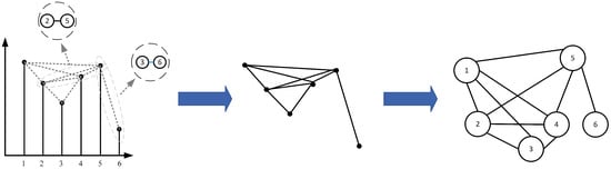
Figure 1.
Visibility graph conversion method.
The primary distinction among HVG, LPVG, and VG lies in their respective visibility criteria, and these visibility graph methods can retain some characteristics of the original time series. However, it is important to acknowledge that these mapping algorithms sequentially evaluate whether each pair of sampling points can form an edge in the graph. This approach results in a time complexity of during algorithmic implementation. Consequently, as the length of the time series extends, the mapping time increases, potentially impacting the program’s runtime significantly. Additionally, these mapping methods are relatively rigid, constructing graphs strictly according to predefined rules; they thus lack flexibility.
While the KNN graph attention method also represents the input feature as a set of unordered nodes , it employs a distinct approach to determine node connectivity. Instead of using a visibility criterion to determine whether two nodes can form an edge, this method utilizes KNN to identify the k nearest neighbors, , of node . It then establishes edges between and each of its nearest neighbors in , where . The KNN graph attention method does not require predefined visualization criteria, unlike the VG method. This lack of rigid criteria enhances both the flexibility and the accuracy of the model’s structure.This is shown in Figure 2. The KNN graph attention method can be expressed as follows:
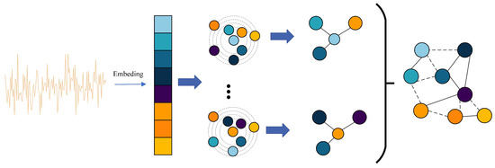
Figure 2.
KNN graph attention method.
For each node, we construct edges to its K nearest neighbors in the current feature space, yielding a KNN graph for message passing. The hyperparameter K controls the receptive field of aggregation: values that are too small restrict information exchange, whereas excessively large values may introduce over-smoothing. Following prior practice in vision GNNs [46], we adopt a progressive schedule in which K increases linearly with depth from i to across the graph blocks. Concretely, for layer ,
which gradually enlarges the neighborhood while keeping early layers stable.
3.2.2. GraphSage (Graph SAmple and aggreGatE)
Previously proposed graph neural network methods, such as GCN, are transductive models that require retraining when changes occur in the network structure, failing to meet the need for rapid real-time generation of network node embeddings. Therefore, we opt to use the inductive model GraphSAGE [47]. The objective of GraphSAGE is to train multiple aggregators that can synthesize the information from neighboring nodes at various distances from the target node, thus quickly generating a low-dimensional vector representation of the unknown node. Its operational process is divided into three steps (Figure 3):
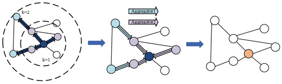
Figure 3.
Process of graph convolution in GraphSage.
- Sample the nodes neighboring each node in the graph
- Aggregate the information contained in all neighboring nodes of the target node according to the aggregation function
- Update the vector representation of each node in the graph for classification
Sampling is done first. For each node, a set number of adjacent nodes, denoted as i, are selected for information aggregation. If the total number of neighboring nodes is less than i, sampling is performed with replacement until i nodes are chosen. Conversely, if the neighborhood exceeds i, sampling proceeds without replacement. The parameter i signifies both the number of network layers and the extent of neighbor hops from which a node can integrate information.
In graph structures, node neighbors are unordered, which requires the development of a symmetric aggregation function. This function must maintain a consistent output regardless of input permutations, ensuring its expressive capability. The inherent symmetry of the aggregation function guarantees that the neural network model can be uniformly trained and applied across any sequence of node neighborhood features, regardless of their order.
We employ a mean aggregator that concatenates the (k − 1)th layer node of the target and neighboring nodes, computes the mean across each vector dimension, and then applies a non-linear transformation to produce the kth layer representation vector for the target node. The mean aggregator function is defined by the following equation:
where denotes the weight of the aggregation function and denotes the GeLU nonlinear activation function. The formula for updating nodes is given by the following equation:
where denotes the weight of the update function.
Traditional GCNs typically employ multiple graph convolution layers to extract aggregated features from data. The phenomenon of excessive smoothing in deep GCNs diminishes the uniqueness of node features, leading to performance degradation in recognizing modulated signals. To mitigate this issue, KGNN incorporates additional linear layers for feature transformation and increased nonlinear activation functions. Specifically, a PWconv layer is integrated both prior to and following graph convolution, facilitating interaction among node features and promoting diversity in feature representation. Nonlinear activation functions are employed post-graph convolution to prevent layer collapse. For a particular input feature X, the updated GraphSage can be expressed as follows:
where and denote the weights of the Conv of the two layers before and after the graph convolution and denotes the GeLU activation function used. denotes the KNN graph attention method used.
3.2.3. FFN
To enhance bolster feature-transformation capabilities and mitigate over-smoothing, KGNN employs a feed-forward network (FFN) following each GraphSage. This FFN module, a straightforward multilayer perceptron, comprises two PWconv layers.
where and are the weights of the PWconv layer. FFNs typically exhibit a rugby-ball-shaped configuration. The BN layer is applied in both GraphSage and FFN and has been omitted for convenience of presentation in the above equations.
An overview of the entire KGNN architecture that integrates these components is shown in Figure 4.
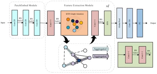
Figure 4.
Overview of the KGNN architecture.
4. Experimental Results
4.1. Dataset and Experimental Environment
In this experiment, we utilized the RML2016.10b dataset, which is a widely recognized standard dataset generated by GNU Radio. To accurately simulate the real channel environment, the dataset incorporates disturbances including additive white Gaussian noise (AWGN), center frequency offset (CFO), and others. The RML2016.10b covers a total of ten modulation types, including two analog modulations (WBFM and AM-DSB) and eight digital modulations (QPSK, BPSK, 8PSK, 64QAM, 16QAM, GFSK, and CPFSK). The database encompasses 1.2 million modulated signals with SNR values uniformly distributed in the range −20 to 18 dB at increments of 2 dB.
Experiments were conducted in Python 3.9 with PyTorch 1.11 on an Intel Core i5-12600KF CPU and an NVIDIA GeForce RTX 3060 (12 GB) GPU. To ensure fair comparison, we fixed the hyperparameters across all runs: 100 epochs, batch size 128, a dynamic learning-rate scheduler with patience = 10, and early stopping with patience = 20. Finally, the end-to-end training and inference workflow is summarized in Algorithm 1.
| Algorithm 1: KGNN: end-to-end training and inference |
 |
4.2. Ablation Experiments
To explore the impact of varying the number of stacked feature-extraction modules on the model, we present our findings with regard to overall accuracy (OA) for different configurations in Figure 5 An OA of 63.7% is achieved with a single layer, demonstrating the significant potential of graph convolution in the AMC domain. As the number of layers increases, overall accuracy generally improves, despite occasional declines, peaking at 64.7% with eight layers. Beyond eight layers, OA begins to decrease slightly, an effect attributed to increased network capacity from additional layering, which can lead to overfitting. Therefore, we opted to use eight layers, as this configuration resulted in the highest accuracy.
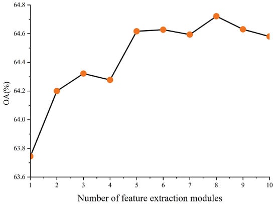
Figure 5.
The effect of multilevel graph structure on classification performance.
To select the initial K for the KNN graph–attention module, we performed an ablation study, as this hyperparameter determines the neighborhood size used to construct the graph and thus directly affects the effectiveness of feature aggregation. We evaluated five candidates, , and measured OA on the RML2016.10b dataset (see Figure 6). Performance increased with larger K at the beginning: OA was for , for , and for . The best result was obtained at , with an OA of . Further increasing to led to a slight drop to . These results indicate that while enlarging the neighborhood initially enriches the information aggregated from local contexts, excessively large K introduces noise and over-smoothing, which degrades classification performance. Accordingly, we adopt as the optimal initial setting in our model.
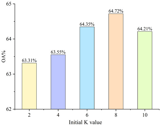
Figure 6.
The impact of the initial K value on the model.
4.3. Classification Properties
To assess the model performance, we compare it with existing models. These include MCLDNN [48], recognized as the best performer; LSTM2 [49], which employs cyclic convolution; AVGNet [42], which utilizes graph convolution; ResNet [50], which is based on standard convolution; and CLDNN [25], which integrates LSTM and CNN. The average accuracy of the modulated signals at each signal-to-noise ratio is illustrated in Figure 7 and Table 1.
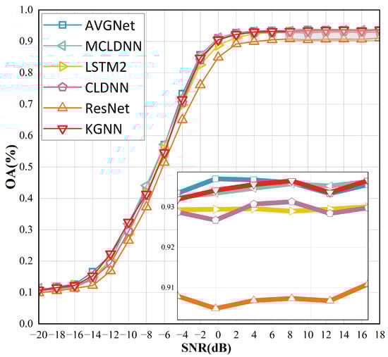
Figure 7.
Accuracy of KGNN on the RML2016.10b dataset at various SNR values.

Table 1.
Overall comparison.
Among the compared methods, KGNN attains the highest OA at 64.72%, narrowly ahead of AVGNet (64.65%) and MCLDNN (64.38%). Moreover, KGNN operates with only one-eighth the number of parameters compared to MCLDNN, and it employs significantly fewer multiply-accumulate operations (MACs). ResNet, with the highest count of trainable parameters at 3 million, exhibits the lowest accuracy, primarily due to its susceptibility to overfitting, which stems from its extensive model capacity. The overall accuracy of LSTM is only 0.2% lower than that of MCLDNN, yet it makes more efficient use of its parameters. Both AVGNet and KGNN, which employ graph convolution, exhibit strong performance in AMC, underscoring graph convolution’s distinct advantages over the regular convolution used by traditional models like ResNet and MCLDNN. This highlights the significant potential of graph convolution in AMC.
The classification performance of the KGNN network across each modulation type is detailed in Table 2. KGNN achieves the highest precision (87%) for QAM64 and the lowest precision (48%) for AM-DSB. KGNN demonstrates superior performance for QAM16 compared to QAM64 in terms of precision, recall, and F1-score. The precision for WBFM is high, while its recall is the lowest.
Table 2.
Accuracy of KGNN on the RML2016b dataset for each modulation type.
4.4. Analysis of Inference Speed
MACs, or Multiply-Accumulate Operations, are the counts of combined multiplication and addition operations. In deep learning models, MACs primarily occur in convolutional layers and fully connected layers. Unlike FLOPs, which count floating-point operations, MACs include both multiplication and addition operations. However, MACs do not fully capture the model’s computational complexity; factors such as the model’s structural design, hardware optimization, and memory access significantly affect the model’s inference time, rendering MACs an indirect measure of computational complexity. A consolidated comparison of parameters, MACs, per-sample inference time, and OA is provided in Table 3. Although our model has fewer parameters compared to others, it does not have the lowest MAC count. This is due to the incorporation of numerous PWconv layers and nonlinear activation functions, which were used to mitigate the over-smoothing effects of graph convolution; this inclusion increases KGNN’s computational load. Compared to AVGNet, which also utilizes graph convolution, KGNN’s computational load is significantly lower. However, this reduction does not substantially impact its accuracy. The MAC of LSTM2 is half that of MCLDNN; however, the negligible difference in inference speed is partly due to the fact that LSTM operations are more time-consuming, and LSTM comprises a disproportionate share of MCLDNN’s inference time. Furthermore, MCLDNN’s multihead parallel operation also contributes significantly to reducing inference time. MCLDNN exhibits the slowest inference speed, partly due to its high computational cost of 49.26 MMAC, and also because of its two-layer LSTM structure, which entails slower operations and thus limits its inference speed. Contrary to expectations, AVGNet’s inference speed is lower than that of KGNN, primarily because the Adaptive Visible Graph (AVG) composition method AVGNet uses includes numerous time-consuming operations, such as one-dimensional convolutions with various kernel sizes, cropping, and splicing. Additionally, AVG’s time consumption escalates dramatically with increases in the length of the input signal. Conversely, KGNN benefits from its KNN graph structure, which is not sensitive to the length of the modulation signal. Additionally, the integration of convolutional layers with batch normalization (BN) layers ensures that the BN layer does not adversely affect KGNN’s inference speed. Recent optimizations in hardware for convolutional layer computations further ensure that KGNN maintains high performance despite its high MAC count.
Table 3.
Overall classification accuracy of each model on RML2016.10b datasets.
4.5. Convergence Analysis
As shown in Figure 8, due to the over-smoothing property of graph convolution, KGNN exhibits significantly slower convergence compared to models like MCLDNN, which are composed of CNNs. In the loss curves, it is evident that KGNN experiences notable fluctuations, which are attributable to the use of a dynamic graph architecture as the backbone feature-extraction module; this structure inherently causes model convergence to fluctuate. Conversely, AVGNet utilizes a fixed graph that employs a convolutional module to compute node-to-node relationships, moving away from the static visualization criteria typically used in VG. This approach allows for adaptive mapping of input modulation signals onto the graph. The adoption of a fixed graph structure minimizes frequent fluctuations during model training. Models such as CLDNN, LSTM, and MCLDNN, which incorporate CNN and LSTM architectures, exhibited stable training with relatively smooth descent curves. In contrast, ResNet displayed a sudden spike in loss at the ninth epoch, likely due to inadequate parameter initialization prior to training.
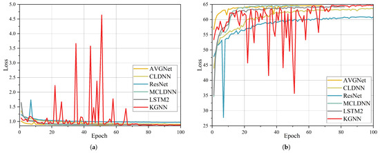
Figure 8.
Convergence of KGNN and other models: (a) validation loss vs. epochs; (b) validation accuracy vs. epochs.
4.6. Confusion Matrix Analysis
Figure 9 presents the confusion matrix at an SNR of 0 dB. KGNN exhibits a comparatively diagonal confusion matrix at 0 dB, indicating fewer systematic misassignments than the baseline models under conditions of strong noise. This suggests that the dynamic, block-wise KNN graph reconstruction—performed from the current features in each block—helps align neighborhoods with the evolving representation, stabilizing aggregation when observations are highly corrupted.
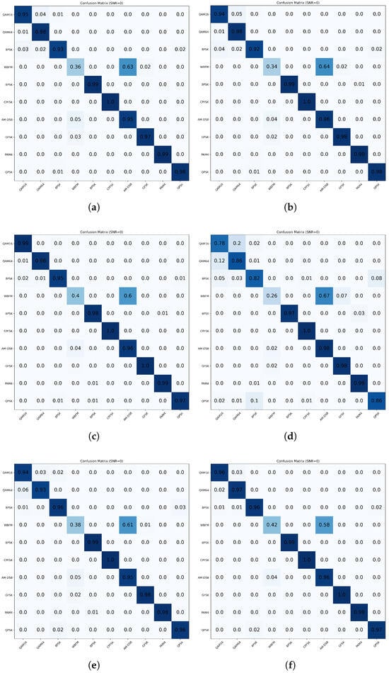
Figure 9.
Confusion matrix for each model at 0 dB SNR on the RML2016b dataset. (a) KGNN. (b) AVGNet. (c) MCLDNN. (d) ResNet. (e) CLDNN. (f) LSTM.
Two confusion pairs dominate the error mass at 0 dB: AM-DSB vs. WBFM among analog classes, likely due to overlapping low-frequency envelopes and similar temporal regularities that become prominent at low SNR, and QAM16 vs. QAM64 among digital classes, where constellation blurring under noise reduces the separability of inner/outer rings.
Compared with AVGNet and MCLDNN, KGNN’s 0 dB matrix contains fewer large off-diagonal blocks for digital modulations, suggesting reduced systematic misalignment. Fixed-graph approaches tend to accumulate persistent analog confusions, and purely convolutional backbones show broader leakage across classes at 0 dB, consistent with limited phase sensitivity or over-smoothing. Models with recurrent components alleviate some temporal errors but still lag behind KGNN in disentangling analog-versus-digital confusions under conditions of strong noise.
5. Conclusions
This work introduced KGNN, a deep learning architecture that encodes modulated signals into 32-dimensional feature nodes, constructs KNN-based graphs from these representations and performs GraphSAGE-driven graph convolution for feature aggregation. The model adopts a dynamic, multi-level graph design with eight stacked feature-extraction modules. On the RML2016.10b dataset, KGNN attains an OA of 64.72%, outperforming conventional graph-based baselines. Moreover, relative to MCLDNN, KGNN reduces the number of parameters used by approximately 87% while maintaining competitive accuracy and faster inference. These results substantiate the effectiveness of dynamic graph structures for AMC and highlight their potential for lightweight deployment. Future work will focus on improving robustness at low SNRs and exploring hybrid CNN–GNN designs to further enhance the accuracy–efficiency trade-off.
Author Contributions
Conceptualization, X.L.; Methodology, X.L.; Software, Z.M.; Validation, Z.M.; Formal analysis, Z.C.; Investigation, M.L.; Resources, M.L.; Data curation, C.W.; Writing—original draft, C.W.; Writing—review & editing, M.L.; Visualization, Z.C.; Supervision, Z.C. All authors have read and agreed to the published version of the manuscript.
Funding
This research received no external funding.
Institutional Review Board Statement
Not applicable.
Informed Consent Statement
Not applicable.
Data Availability Statement
The original data presented in this study are openly available in the RadioML 2016.10b dataset at the DeepSig Datasets portal (https://www.deepsig.ai/datasets; accessed on 28 October 2025).
Conflicts of Interest
The authors declare no conflicts of interest.
List of Abbreviations
The following abbreviations are used in the manuscript to improve clarity and facilitate cross-referencing.
| AM-DSB | Amplitude Modulation—Double Sideband |
| AMC | Automatic Modulation Classification |
| AP | Amplitude–Phase |
| AVGNet | Adaptive Visibility Graph Neural Network |
| AWGN | Additive White Gaussian Noise |
| BPSK | Binary Phase Shift Keying |
| BN | Batch Normalization |
| CNN | Convolutional Neural Network |
| CLDNN | CNN–LSTM–DNN hybrid |
| CPFSK | Continuous-Phase Frequency Shift Keying |
| DNN | Deep Neural Network |
| FFN | Feed-Forward Network |
| GAN | Generative Adversarial Network |
| GCN | Graph Convolutional Network |
| GeLU | Gaussian Error Linear Unit |
| GFSK | Gaussian Frequency Shift Keying |
| GNN | Graph Neural Network |
| GraphSAGE | Graph Sample and Aggregate |
| GRU | Gated Recurrent Unit |
| HVG | Horizontal Visibility Graph |
| IQ | In-phase/Quadrature |
| KGNN | KNN + GraphSAGE Graph Neural Network |
| KNN | k-Nearest Neighbors |
| LSTM | Long Short-Term Memory |
| LPVG | Limited Penetrable Visibility Graph |
| MACs | Multiply–Accumulate Operations |
| MCLDNN | Multi-Channel LSTM + CNN + DNN |
| OA | Overall Accuracy |
| PAM4 | 4-Level Pulse Amplitude Modulation |
| PWConv | Pointwise Convolution (1 × 1) |
| QAM16 | 16-Quadrature Amplitude Modulation |
| QAM64 | 64-Quadrature Amplitude Modulation |
| QPSK | Quadrature Phase Shift Keying |
| RML2016.10b | RadioML 2016.10b |
| RNN | Recurrent Neural Network |
| ResNet | Residual Network |
| SE | Squeeze-and-Excitation |
| SNR | Signal-to-Noise Ratio |
| TCN | Temporal Convolutional Network |
| VG | Visibility Graph |
| WBFM | Wideband Frequency Modulation |
References
- Jiang, W.; Han, B.; Habibi, M.A.; Schotten, H.D. The road towards 6G: A comprehensive survey. IEEE Open J. Commun. Soc. 2021, 2, 334–366. [Google Scholar] [CrossRef]
- Tang, F.; Kawamoto, Y.; Kato, N.; Liu, J. Future intelligent and secure vehicular network toward 6G: Machine-learning approaches. Proc. IEEE 2019, 108, 292–307. [Google Scholar] [CrossRef]
- Guo, F.; Yu, F.R.; Zhang, H.; Li, X.; Ji, H.; Leung, V.C. Enabling massive IoT toward 6G: A comprehensive survey. IEEE Internet Things J. 2021, 8, 11891–11915. [Google Scholar] [CrossRef]
- Zhu, Z.; Nandi, A.K. Modulation classification in MIMO fading channels via expectation maximization with non-data-aided initialization. In Proceedings of the 2015 IEEE International Conference on Acoustics, Speech and Signal Processing (ICASSP), South Brisbane, Australia, 19–24 April 2015; pp. 3014–3018. [Google Scholar]
- Hameed, F.; Dobre, O.A.; Popescu, D.C. On the likelihood-based approach to modulation classification. IEEE Trans. Wirel. Commun. 2009, 8, 5884–5892. [Google Scholar] [CrossRef]
- Ramezani-Kebrya, A.; Kim, I.M.; Kim, D.I.; Chan, F.; Inkol, R. Likelihood-based modulation classification for multiple-antenna receiver. IEEE Trans. Commun. 2013, 61, 3816–3829. [Google Scholar] [CrossRef]
- Liedtke, F. Computer simulation of an automatic classification procedure for digitally modulated communication signals with unknown parameters. Signal Process. 1984, 6, 311–323. [Google Scholar] [CrossRef]
- Azzouz, E.E.; Nandi, A.K. Automatic identification of digital modulation types. Signal Process. 1995, 47, 55–69. [Google Scholar] [CrossRef]
- Nishani, E.; Çiço, B. Computer vision approaches based on deep learning and neural networks: Deep neural networks for video analysis of human pose estimation. In Proceedings of the 2017 6th Mediterranean Conference on Embedded Computing (MECO), Bar, Montenegro, 11–15 June 2017; pp. 1–4. [Google Scholar]
- Wang, P. Research and design of smart home speech recognition system based on deep learning. In Proceedings of the 2020 International Conference on Computer Vision, Image and Deep Learning (CVIDL), Chongqing, China, 10–12 July 2020; pp. 218–221. [Google Scholar]
- Dong, Y.N.; Liang, G.S. Research and discussion on image recognition and classification algorithm based on deep learning. In Proceedings of the 2019 International Conference on Machine Learning, Big Data and Business Intelligence (MLBDBI), Taiyuan, China, 8–10 November 2019; pp. 274–278. [Google Scholar]
- Zunjani, F.H.; Sen, S.; Shekhar, H.; Powale, A.; Godnaik, D.; Nandi, G. Intent-based object grasping by a robot using deep learning. In Proceedings of the 2018 IEEE 8th International Advance Computing Conference (IACC), Greater Noida, India, 14–15 December 2018; pp. 246–251. [Google Scholar]
- Huynh-The, T.; Pham, Q.V.; Nguyen, T.V.; Nguyen, T.T.; Ruby, R.; Zeng, M.; Kim, D.S. Automatic modulation classification: A deep architecture survey. IEEE Access 2021, 9, 142950–142971. [Google Scholar] [CrossRef]
- Kim, B.; Kim, J.; Chae, H.; Yoon, D.; Choi, J.W. Deep neural network-based automatic modulation classification technique. In Proceedings of the 2016 International Conference on Information and Communication Technology Convergence (ICTC), Jeju, Republic of Korea, 19–21 October 2016; pp. 579–582. [Google Scholar]
- O’Shea, T.J.; Corgan, J.; Clancy, T.C. Convolutional radio modulation recognition networks. In Engineering Applications of Neural Networks, Proceedings of the 17th International Conference, EANN 2016, Aberdeen, UK, 2–5 September 2016; Proceedings 17; Springer: Cham, Switzerland, 2016; pp. 213–226. [Google Scholar]
- Hong, S.; Zhang, Y.; Wang, Y.; Gu, H.; Gui, G.; Sari, H. Deep learning-based signal modulation identification in OFDM systems. IEEE Access 2019, 7, 114631–114638. [Google Scholar] [CrossRef]
- Chang, S.; Huang, S.; Zhang, R.; Feng, Z.; Liu, L. Multitask-learning-based deep neural network for automatic modulation classification. IEEE Internet Things J. 2021, 9, 2192–2206. [Google Scholar] [CrossRef]
- Zheng, Q.; Tian, X.; Yu, Z.; Yang, M.; Elhanashi, A.; Saponara, S. Robust automatic modulation classification using asymmetric trilinear attention net with noisy activation function. Eng. Appl. Artif. Intell. 2025, 141, 109861. [Google Scholar] [CrossRef]
- Ouamna, H.; Kharbouche, A.; Madini, Z.; Zouine, Y. Deep Learning-assisted Automatic Modulation Classification using Spectrograms. Eng. Technol. Appl. Sci. Res. 2025, 15, 19925–19932. [Google Scholar] [CrossRef]
- Tian, X.; Chen, C. Modulation pattern recognition based on Resnet50 neural network. In Proceedings of the 2019 IEEE 2nd International Conference on Information Communication and Signal Processing (ICICSP), Weihai, China, 28–30 September 2019; pp. 34–38. [Google Scholar]
- Mao, Y.; Ren, W.; Yang, Z. Radar signal modulation recognition based on sep-ResNet. Sensors 2021, 21, 7474. [Google Scholar] [CrossRef] [PubMed]
- Chen, Y.; Shao, W.; Liu, J.; Yu, L.; Qian, Z. Automatic modulation classification scheme based on LSTM with random erasing and attention mechanism. IEEE Access 2020, 8, 154290–154300. [Google Scholar] [CrossRef]
- Daldal, N.; Sengur, A.; Polat, K.; Cömert, Z. A novel demodulation system for base band digital modulation signals based on the deep long short-term memory model. Appl. Acoust. 2020, 166, 107346. [Google Scholar] [CrossRef]
- Wang, Y.; Zhang, H.; Xu, L.; Cao, C.; Gulliver, T.A. Adoption of hybrid time series neural network in the underwater acoustic signal modulation identification. J. Frankl. Inst. 2020, 357, 13906–13922. [Google Scholar] [CrossRef]
- West, N.E.; O’shea, T. Deep architectures for modulation recognition. In Proceedings of the 2017 IEEE International Symposium on Dynamic Spectrum Access Networks (DySPAN), Baltimore, MD, USA, 6–9 March 2017; pp. 1–6. [Google Scholar]
- Njoku, J.N.; Morocho-Cayamcela, M.E.; Lim, W. CGDNet: Efficient hybrid deep learning model for robust automatic modulation recognition. IEEE Netw. Lett. 2021, 3, 47–51. [Google Scholar] [CrossRef]
- Chen, S.; Zhang, Y.; He, Z.; Nie, J.; Zhang, W. A novel attention cooperative framework for automatic modulation recognition. IEEE Access 2020, 8, 15673–15686. [Google Scholar] [CrossRef]
- Huang, S.; Dai, R.; Huang, J.; Yao, Y.; Gao, Y.; Ning, F.; Feng, Z. Automatic modulation classification using gated recurrent residual network. IEEE Internet Things J. 2020, 7, 7795–7807. [Google Scholar] [CrossRef]
- Ouamna, H.; Kharbouche, A.; El-Haryqy, N.; Madini, Z.; Zouine, Y. Performance Analysis of a Hybrid Complex-Valued CNN-TCN Model for Automatic Modulation Recognition in Wireless Communication Systems. Appl. Syst. Innov. 2025, 8, 90. [Google Scholar] [CrossRef]
- El-Haryqy, N.; Kharbouche, A.; Ouamna, H.; Madini, Z.; Zouine, Y. Improved automatic modulation recognition using deep learning with additive attention. Results Eng. 2025, 26, 104783. [Google Scholar] [CrossRef]
- Chen, Y.; Dong, B.; Liu, C.; Xiong, W.; Li, S. Abandon locality: Frame-wise embedding aided transformer for automatic modulation recognition. IEEE Commun. Lett. 2022, 27, 327–331. [Google Scholar] [CrossRef]
- Zhang, L.; Lambotharan, S.; Zheng, G.; Liao, G.; AsSadhan, B.; Roli, F. Attention-based adversarial robust distillation in radio signal classifications for low-power IoT devices. IEEE Internet Things J. 2022, 10, 2646–2657. [Google Scholar] [CrossRef]
- Liu, X. Automatic modulation classification based on improved R-Transformer. In Proceedings of the 2021 International Wireless Communications and Mobile Computing (IWCMC), Harbin, China, 28 June–2 July 2021; pp. 1–8. [Google Scholar]
- Liang, Z.; Tao, M.; Xie, J.; Yang, X.; Wang, L. A radio signal recognition approach based on complex-valued CNN and self-attention mechanism. IEEE Trans. Cogn. Commun. Netw. 2022, 8, 1358–1373. [Google Scholar] [CrossRef]
- Zhang, M.; Cui, Z.; Neumann, M.; Chen, Y. An end-to-end deep learning architecture for graph classification. In Proceedings of the 32nd AAAI Conference on Artificial Intelligence, New Orleans, LA, USA, 2–7 February 2018; Volume 32. [Google Scholar]
- Ying, Z.; You, J.; Morris, C.; Ren, X.; Hamilton, W.; Leskovec, J. Hierarchical graph representation learning with differentiable pooling. In Proceedings of the Advances in Neural Information Processing Systems 31 (NeurIPS 2018), Montreal, QC, Canada, 3–8 December 2018; Volume 31. [Google Scholar]
- Lee, J.; Lee, I.; Kang, J. Self-attention graph pooling. In Proceedings of the 36th International Conference on Machine Learning, Long Beach, CA, USA, 9–15 June 2019; pp. 3734–3743. [Google Scholar]
- Yan, X.; Zhang, G.; Wu, H.C. A Novel Automatic Modulation Classifier Using Graph-Based Constellation Analysis for M-ary QAM. IEEE Commun. Lett. 2018, 23, 298–301. [Google Scholar] [CrossRef]
- Zhang, Q.; Ji, H.; Li, L.; Zhu, Z. Automatic Modulation Recognition of Unknown Interference Signals Based on Graph Model. IEEE Wirel. Commun. Lett. 2024, 13, 2317–2321. [Google Scholar] [CrossRef]
- Qiu, K.; Zheng, S.; Zhang, L.; Lou, C.; Yang, X. Deepsig: A hybrid heterogeneous deep learning framework for radio signal classification. IEEE Trans. Wirel. Commun. 2023, 23, 775–788. [Google Scholar] [CrossRef]
- Suetrong, N.; Taparugssanagorn, A.; Promsuk, N. Enhanced Modulation Recognition Through Deep Transfer Learning in Hybrid Graph Convolutional Networks. IEEE Access 2024, 12, 54553–54566. [Google Scholar] [CrossRef]
- Xuan, Q.; Zhou, J.; Qiu, K.; Chen, Z.; Xu, D.; Zheng, S.; Yang, X. AvgNet: Adaptive visibility graph neural network and its application in modulation classification. IEEE Trans. Netw. Sci. Eng. 2022, 9, 1516–1526. [Google Scholar] [CrossRef]
- Ghasemzadeh, P.; Hempel, M.; Sharif, H. A robust graph convolutional neural network-based classifier for automatic modulation recognition. In Proceedings of the 2022 International Wireless Communications and Mobile Computing (IWCMC), Dubrovnik, Croatia, 30 May–3 June 2022; pp. 907–912. [Google Scholar]
- Zhu, H.; Xu, H.; Shi, Y.; Zhang, Y.; Jiang, L. A Modulation Classification Algorithm Based on Feature-Embedding Graph Convolutional Network. IEEE Access 2024, 13, 125057–125065. [Google Scholar] [CrossRef]
- Lacasa, L.; Luque, B.; Ballesteros, F.; Luque, J.; Nuno, J.C. From time series to complex networks: The visibility graph. Proc. Natl. Acad. Sci. USA 2008, 105, 4972–4975. [Google Scholar] [CrossRef] [PubMed]
- Han, K.; Wang, Y.; Guo, J.; Tang, Y.; Wu, E. Vision gnn: An image is worth graph of nodes. Adv. Neural Inf. Process. Syst. 2022, 35, 8291–8303. [Google Scholar]
- Leskovec, J. GraphSAGE: Inductive Representation Learning on Large Graphs; SNAP: Long Beach, CA, USA, 2020.
- Xu, J.; Luo, C.; Parr, G.; Luo, Y. A spatiotemporal multi-channel learning framework for automatic modulation recognition. IEEE Wirel. Commun. Lett. 2020, 9, 1629–1632. [Google Scholar] [CrossRef]
- Rajendran, S.; Meert, W.; Giustiniano, D.; Lenders, V.; Pollin, S. Deep learning models for wireless signal classification with distributed low-cost spectrum sensors. IEEE Trans. Cogn. Commun. Netw. 2018, 4, 433–445. [Google Scholar] [CrossRef]
- Liu, X.; Yang, D.; El Gamal, A. Deep neural network architectures for modulation classification. In Proceedings of the 2017 51st Asilomar Conference on Signals, Systems, and Computers, Pacific Grove, CA, USA, 29 October–1 November 2017; pp. 915–919. [Google Scholar]


Disclaimer/Publisher’s Note: The statements, opinions and data contained in all publications are solely those of the individual author(s) and contributor(s) and not of MDPI and/or the editor(s). MDPI and/or the editor(s) disclaim responsibility for any injury to people or property resulting from any ideas, methods, instructions or products referred to in the content. |
© 2025 by the authors. Licensee MDPI, Basel, Switzerland. This article is an open access article distributed under the terms and conditions of the Creative Commons Attribution (CC BY) license (https://creativecommons.org/licenses/by/4.0/).