Daily Peak Load Prediction Method Based on XGBoost and MLR

Abstract

During the peak load period, there is a high level of imbalance between power supply and demand, which has become a critical challenge, leading to higher operational costs for power grids. To improve the accuracy of peak load forecasting, this study introduces a novel approach based on Extreme Gradient Boosting Trees (XGBoost) and Multiple Linear Regression (MLR) for daily peak load prediction. The proposed methodology first employs an improved version of the Complete Ensemble Empirical Mode Decomposition with Adaptive Noise (ICEEMDAN) algorithm to decompose the raw load data, subsequently reconstructing each Intrinsic Mode Function (IMF) into high-frequency and stationary components. For the high-frequency components, XGBoost serves as the base predictor within a Bagging-based ensemble structure, while the Sparrow Search Algorithm (SSA) is employed to optimize hyperparameters automatically, ensuring efficient learning and accurate representation of complex peak load fluctuations. Meanwhile, the stationary components are modeled using MLR to provide fast and reliable estimations. The proposed framework was evaluated using actual daily peak load data from Western Inner Mongolia, China. The results indicate that the proposed method successfully captures the peak characteristics of the power grid, delivering both robust and precise predictions. When compared to the baseline model, the RMSE and MAPE are reduced by 54.4% and 87.3%, respectively, underscoring its significant potential for practical applications in power system operation and planning.

1. Introduction

The issue of power supply and demand imbalance during peak load periods has become increasingly prominent, leading to higher operational costs for power grids [1,2]. Accurate peak load forecasting directly impacts capacity planning, equipment maintenance, and emergency response strategies [3,4]. Inaccurate peak load predictions can lead to grid overload or resource waste, and in severe cases, it can even trigger power outages and grid failures. Moreover, peak load forecasting plays a crucial role in calculating reserve capacities, implementing demand response measures, and determining peak and off-peak electricity pricing [5]. This issue is particularly significant during summer and winter peak demand periods, when the gap between supply and demand is substantial [6]. For instance, in September 2021, large-scale power outages occurred in Northeast China and other provinces, primarily due to power shortages that could not meet the rapidly growing electricity demand. Therefore, accurately forecasting peak loads in the coming days would help the grid develop scheduling plans, assist power companies in formulating production plans, and narrow the supply–demand gap. Furthermore, accurate peak load forecasting is vital for ensuring the safe and stable operation of grids in regions with weak grid structures and heavy loads.

Currently, peak load forecasting methods can be broadly categorized into statistical analysis, machine learning, and model-based forecasting using load characteristics analysis. Reference [7] summarizes the impact of the day of the week and month on peak loads and proposes a hybrid forecasting model using the Differencing Integrated Moving Average Regression model to predict grid loads. Reference [8] utilizes robust regression methods to forecast peak loads. Reference [9] introduces a short-term load forecasting method based on improved empirical mode decomposition and neural networks, effectively improving forecasting accuracy. Reference [10] decomposes monthly electricity consumption into non-periodic trend components and seasonal components using seasonal indices to model the time-varying load. Reference [11] analyzes the impact of regional weather variables on grid loads and uses alternating conditional expectation nonparametric simulation for peak load forecasting. Although these methods have yielded good results, they still have some limitations. Firstly, traditional statistical methods are ineffective at capturing dynamic load changes when dealing with large volumes of high-dimensional grid data. Secondly, although machine learning and load characteristic-based methods can theoretically handle complex data relationships, their practical application is often constrained by data quality. Moreover, most of the studies cited above utilize single models, which tend to become trapped in local minima during training. As a result, models that correspond to these local optima often struggle with generalization.

Over the past few years, deep neural network algorithms have been increasingly applied to power grid peak load forecasting. The error backpropagation network in References [12,13] is widely used and capable of implementing complex nonlinear mappings between inputs and outputs. Reference [14] proposes a method for short- and long-term peak load forecasting at the regional level. Reference [15] uses a gray prediction method to forecast short-term peak loads. Reference [16] applies CNN-LSTM models for short-term load forecasting, validated using data from the Bangladesh power system. Reference [17] first decomposes the raw load data into several Intrinsic Mode Functions (IMFs) using EEMD and constructs a hybrid neural network based on DBN and BILSTM to predict daily peak loads for the following month. Reference [18] constructs a deep hybrid network using CNN, GRU, and Fully Connected Layers (FCNs). However, deep learning networks have complex architectures, and the selection of hidden layers and node numbers greatly influences training outcomes. If poorly designed, the network often falls into local minima and overfitting. These characteristics limit the further development of deep learning in load forecasting.

In recent years, substantial advancements have been made in tree ensemble algorithms. Notably, in competitive environments such as the Kaggle data science competition, tree ensemble algorithms, particularly XGBoost, have demonstrated superior performance, surpassing many deep learning models. Reference [19] leverages the XGBoost algorithm to mitigate overfitting, successfully predicting the cooling and heating loads of buildings. In a similar vein, Reference [20] integrates the Bagging algorithm with XGBoost, employing the Particle Swarm Optimization (PSO) algorithm to fine-tune XGBoost’s hyperparameters. Reference [21] adopts genetic algorithms (GAs) to further optimize the hyperparameters of XGBoost. While these intelligent optimization algorithms are effective in refining deep neural networks, they often suffer from slow convergence rates and a propensity to converge to local optima. In contrast, the Sparrow Search Optimization Algorithm (SSA) draws inspiration from the collective behaviors of sparrows during predation and anti-predation processes, utilizing their cooperative and competitive dynamics to explore and identify optimal solutions. SSA excels in both efficiency and precision, particularly in parameter optimization, thus overcoming many of the shortcomings typically encountered in traditional optimization methods. Consequently, SSA has emerged as a promising optimization tool, particularly for enhancing the performance of machine learning and deep learning models [22,23].

To tackle the challenges outlined, we propose a new peak load forecasting model that combines XGBoost with multiple linear regression (MLR). A comparison between our approach and the latest research is presented in

Table 1. A comparison between our approach and the latest research.

Ref.	Hybrid Model	Tree Ensemble Algorithm	Heuristic Algorithm
[7]	×	√	×
[8,9,10,11]	×	×	×
[12,13]	√	×	×
[14]	×	×	×
[19]	√	√	×
[20]	√	√	PSO
[21]	√	√	GA
Proposed	√	√	SSA

The cross and checkmark indicate the absence and presence of the method, respectively.

. Initially, historical load data is subjected to decomposition using the ICEEMDAN algorithm, which separates the data into high-frequency and stationary components. To predict the high-frequency components, Bagging-XGBoost is employed, and the Sparrow Search Optimization Algorithm (SSA) is incorporated to optimize the hyperparameters of XGBoost, thereby reducing the computational time required for this process. For the stationary components, MLR is utilized, taking advantage of its robust curve fitting capabilities and computational efficiency to deliver accurate predictions. Subsequently, the output from the first-layer model is fed into the second-layer prediction model, which consists of SSA-XGBoost, for nonlinear fusion and reconstruction. This final step results in the generation of the ultimate peak load prediction.

2. Overall Framework of Peak Load Forecasting Model

Due to factors such as seasonal variations, diurnal differences, and the diversity of load patterns, electrical load data typically exhibit both periodic and fluctuating characteristics [24]. This is especially true for peak load forecasting scenarios over multiple consecutive days or even an entire month. If the predictive model directly learns from the raw peak load sequences, it will be significantly affected by data disturbances during training, leading to poor model generalization and robustness [25]. Therefore, to reduce the nonlinearity in peak load sequences, simplify the prediction task, and improve prediction accuracy, this study proposes a daily peak load forecasting method based on XGBoost and MLR. The overall framework of the two-layer continuous multi-day peak load forecasting model, based on ICEEMDAN-Bagging-XGBoost-MLR, proposed in this paper is shown in Figure 1. The model analysis and algorithm flow will be described in detail below.

In this study, the original peak load sequence is subjected to decomposition using the ICEEMDAN algorithm, which separates the data into distinct high-frequency and stationary components based on the zero-crossing rate of each Intrinsic Mode Function (IMF). For the high-frequency components, which encapsulate the detailed fluctuations in peak load and exhibit considerable randomness, the SSA-Bagging-XGBoost method is utilized for prediction. This methodology effectively mitigates variance and bias throughout the training process, facilitating a more accurate tracking of the load change curve. In contrast, for the low-frequency stationary components, which primarily capture the overall load variation trends, Multiple Linear Regression (MLR) is employed for prediction. The simplicity of the MLR model, combined with its strong curve fitting capability and reduced susceptibility to overfitting, makes it well-suited to this task.

Specifically, we first evaluate the contribution of each input feature to the model using the tree gain metrics derived from the XGBoost and Random Forest (RF) algorithms. These selected features are then used to define the final input set for the prediction model. The high-frequency and stationary components produced by the decomposition process serve as the target outputs. When combined with the identified input features, this forms the dataset required by the model. Next, using this dataset, the SSA optimization algorithm is applied to search for the optimal hyperparameters for XGBoost (such as the number of trees, tree depth, learning rate, and the minimum loss for node splitting). Afterward, under the optimal hyperparameter configuration, the initial training samples are fed into the Bagging-XGBoost model to predict the high-frequency components. In contrast, MLR does not require hyperparameter tuning and can directly predict the stationary components using the validation and test sets after training.

3. Framework Modules

3.1. ICEEMDAN Algorithm Mechanism

The Empirical Mode Decomposition (EMD) method is widely used for processing non-stationary and nonlinear signals. Essentially, it smooths the signal and decomposes the complex original signal into several Intrinsic Mode Functions (IMFs), ordered by their frequencies from high to low. However, a phenomenon known as modal aliasing arises during the decomposition process of the EMD algorithm. Although the Ensemble Empirical Mode Decomposition (EEMD) algorithm addresses the issue of mode aliasing in EMD, it leaves a certain amount of white noise in the IMF components, which increases reconstruction errors. In comparison to EEMD, the Complete Ensemble Empirical Mode Decomposition with Adaptive Noise (CEEMDAN) algorithm further reduces reconstruction errors by adding adaptive white noise. As an improvement to CEEMDAN, the Improved Complete Ensemble Empirical Mode Decomposition with Adaptive Noise (ICEEMDAN) algorithm directly introduces Gaussian white noise ($E_k\left(w^{\left(i\right)}\right)$) during the decomposition process. It then decomposes the white noise using EMD and selects the k-th IMF component to further eliminate residual noise from the IMF components and reduce the occurrence of spurious modal components. The decomposition process is well-documented in the literature [26].

3.2. XGBoost Algorithm Mechanism

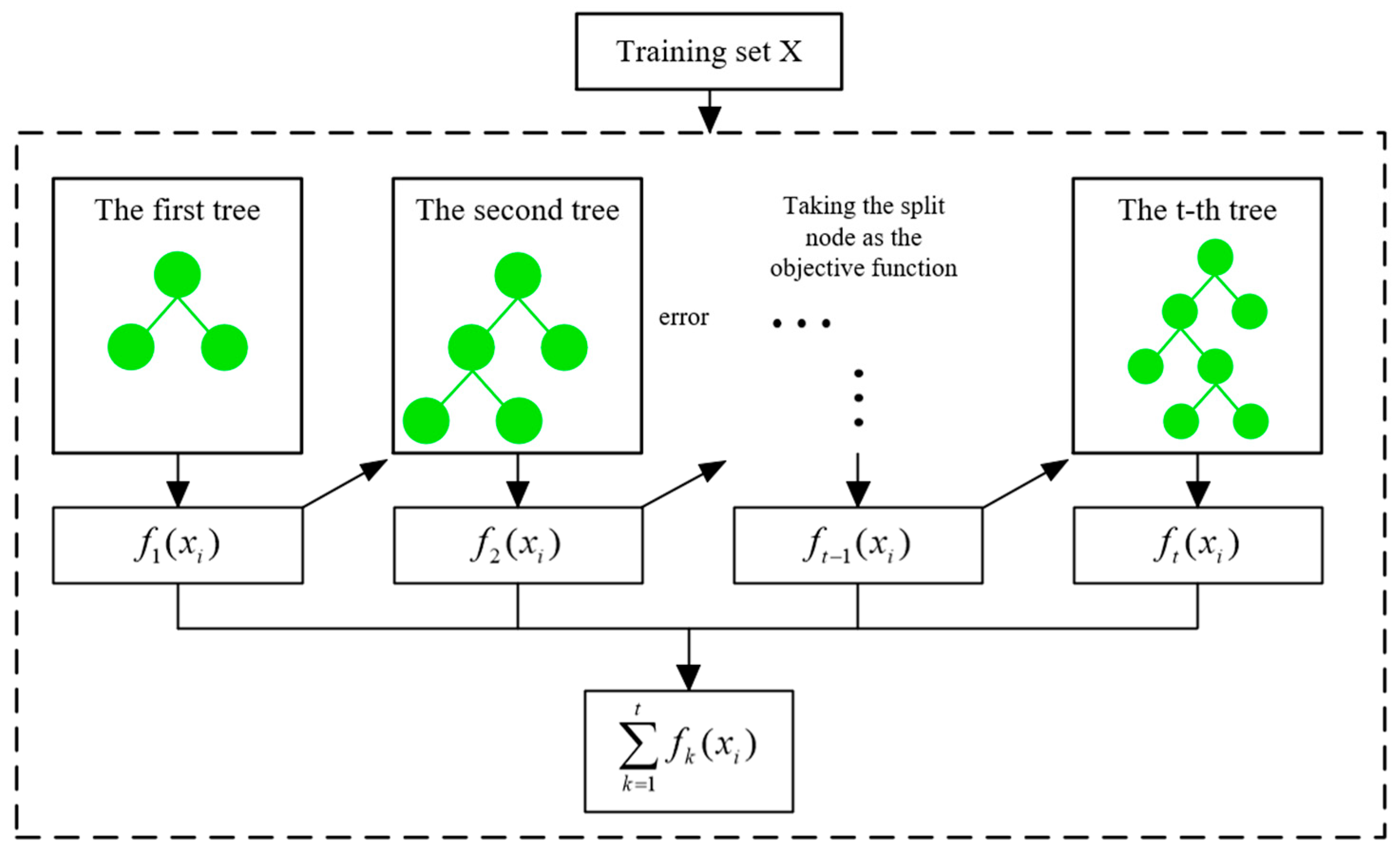
XGBoost is an ensemble learning-based tree boosting model. The idea behind it is to iteratively add different trees to the model, where each tree grows through feature splitting and fits the residuals of the predictions from all previous trees. Its learning mechanism is shown in Figure 2.

For the dataset $D=\left\{\left(x_i,y_i\right)\right\}$, ($\left|D\right|=n$), the ensemble model is expressed as follows.

$${\widehat{y_i}}^{\left(t\right)}=\sum _{k=1}^t{f}_k\left(x_i\right)={\widehat{y_i}}^{\left(t-1\right)}+f_t\left(x_i\right)$$

(1)

where ${\widehat{y_i}}^{\left(t\right)}$ is the prediction result, ${\widehat{y_i}}^{\left(t-1\right)}$ is the sum of the prediction results, and $f_t\left(x_i\right)$ is the newly added tree.

The loss function of XGBoost consists of two parts: the prediction error and the regularization term.

$${Obj}^{\left(t\right)}=\sum _{i=1}^{n}l\left(y_i,{\widehat{y_i}}^{\left(t-1\right)}+f_t\left(x_i\right)\right)+\sum _{i=1}^t\mathsf{\Omega }\left(f_t\right)$$

(2)

$$\mathsf{\Omega }\left(f_t\right)=\gamma T+{\displaystyle \frac{1}{2}}\lambda {‖w‖}^2$$

(3)

where $\gamma$ and $\lambda$ are the penalty coefficients, $T$ is the number of leaves in the tree, and $w$ is the leaf weight. Since the complexity of the first t − 1 trees is a known constant, Equation (2) can be rewritten as:

$${Obj}^{\left(t\right)}=\sum _{i=1}^{n}l\left(y_i,{\widehat{y_i}}^{\left(t-1\right)}+f_t\left(x_i\right)\right)+\mathsf{\Omega }\left(f_t\right)+constant$$

(4)

The loss function is expanded using a second-order Taylor series, yielding:

$${Obj}^{\left(t\right)}\cong \sum _{i=1}^n\left[l\left(y_i,{\widehat{y_i}}^{\left(t-1\right)}\right)+g_i{f}_t\left(x_i\right)+{\displaystyle \frac{1}{2}}{h}_i{f_t}^2\left(x_i\right)\right]+\mathsf{\Omega }\left(f_t\right)+constant$$

(5)

$$\left\{\begin{array}{c}{\widehat{y_i}}^{\left(0\right)}=0\\ {\widehat{y_i}}^{\left(1\right)}=f_1\left(x_i\right)={\widehat{y_i}}^{\left(0\right)}+f_1\left(x_i\right)\\ {\widehat{y_i}}^{\left(2\right)}=f_1\left(x_i\right)+f_2\left(x_i\right)={\widehat{y_i}}^{\left(1\right)}+f_2\left(x_i\right)\\ ⋮\\ {\widehat{y_i}}^t={\displaystyle \sum _{k=1}^t}{f}_k\left(x_i\right)={\widehat{y_i}}^{\left(t\right)}+f_t\left(x_i\right)\end{array}\right.$$

(6)

where $g_i={\partial }_{{\widehat{y_i}}^{\left(t-1\right)}}l\left(y_i,{\widehat{y_i}}^{\left(t-1\right)}\right)$, $h_i={\partial }_{{\widehat{y_i}}^{\left(t-1\right)}}^{2}l\left(y_i,{\widehat{y_i}}^{\left(t-1\right)}\right)$.

The incremental training method adopted by the XGBoost algorithm is that in each iteration, new trees are continuously added to fit the previous error value to reduce the objective function as much as possible, as shown in Equation (7).

$${Obj}^{\left(t\right)}\cong \sum _{i=1}^n\left[g_i{f}_t\left(x_i\right)+{\displaystyle \frac{1}{2}}{h}_i{f_t}^2\left(x_i\right)\right]+\mathsf{\Omega }\left(f_t\right)$$

(7)

3.3. Multiple Linear Regression Mechanism

Multiple linear regression (MLR) is a traditional mathematical statistical model with early development, simple model and fast calculation speed, which has a good fitting effect on smooth curves. MLR is very suitable for forecasting data with strong periodicity and relatively stable, and its formula is:

$$Y=X\times \beta +\mu$$

(8)

where Y is the target output matrix; X is the input feature matrix; $\beta$ is the retrospective coefficient matrix; $\mu$ is a constant term. For the regression parameters, the least squares method is used to estimate them, and the regression function can be obtained. The formula is:

$$\widehat{\beta }={\left(X^{\prime }X\right)}^{-1}{X}^{\prime }Y$$

(9)

3.4. Parallel Ensemble Learning Method of Bagging Mechanism

Bagging is an ensemble learning technique designed to effectively reduce variance. As shown in Figure 3, the algorithm’s architecture follows a self-sampling method (Bootstrap) to generate multiple random datasets. For instance, given a dataset D with m samples, random sampling with replacement is applied to produce a new dataset $D_i$ containing the same number of samples as the original dataset, performed m times. This process results in duplicate samples within the new dataset due to the random sampling. After completing n iterations of this self-sampling process, n new datasets $\left\{D_1,D_2,\cdots D_{n-1},D_n\right\}$ are obtained. Each dataset is used to train n independent base learners $\left\{V_1,V_2,\cdots V_{n-1},V_n\right\}$. In regression tasks, the outputs from the trained base learners are averaged to compute the final result.

3.5. Sparrow Search Optimization Algorithm Mechanism

The Sparrow Search Optimization Algorithm (SSA) is an innovative swarm intelligence optimization technique inspired by the foraging and anti-predation behaviors of sparrows. Within the SSA framework, three distinct roles are defined: the discoverer, the joiner, and the predator. In an N-dimensional search space, the position of the i-th sparrow is represented as follows:

$${X_i}^t=\left\{x_{i,1}^t,x_{i,2}^t,\cdots {,x}_{i,N}^t\right\},i=\mathrm{1,2},\cdots m$$

(10)

where $t$ is the current iteration number; $m$ is the population size.

The position update formula for the discoverer within the sparrow population is given by:

$$x_{i,j}^{t+1}=\left\{\begin{array}{c}\sigma \exp \left(-{\displaystyle \frac{x_{worse}^t-x_{i,j}^t}{i^2}}\right),i>n/2\\ x_{best}^{t+1}+{\displaystyle \frac{1}{N}}{\displaystyle \sum _j^N}\left(rand\left\{-1,1\right\}·\left|x_{i,j}^t-x_{best}^{t+1}\right|\right),i\le n/2\end{array}\right.$$

(11)

where $x_{i,j}^t$ represents the position of the sparrow, $x_{worse}^t$ denotes the worst solution on the j-th dimension of the current population’s search space, and $x_{best}^{t+1}$ corresponds to the optimal solution on the j-th dimension in the search space for the current population. When i > n/2, it indicates that the i-th joiner has not found a better solution and decides to explore other areas. Conversely, when i ≤ n/2, the joiner will monitor the discoverer, competing for the best solution, and may replace the discoverer to explore a larger search space.

Additionally, the sparrow search algorithm includes predators, whose positions are determined as follows:

$$x_{i,j}^{t+1}=\left\{\begin{array}{c}{x}_{best}^t+\beta \left|x_{i,j}^t-x_{best}^t\right|,f_i\ne f_{best}\\ x_{i,j}^t+K\left({\displaystyle \frac{\left|x_{i,j}^t-x_{worse}^t\right|}{\left(f_i-f_{worse}\right)+\mu }}\right),f_i=f_{best}\end{array}\right.$$

(12)

where $\beta$ is a random variable following a standard normal distribution, $K\in [-1,1]$, and $\mu$ is a small constant to prevent the denominator from becoming zero. $f_{worse}$ and $f_{best}$ represent the worst and optimal fitness values of the current population, respectively, while $f_i$ denotes the fitness value of the i-th sparrow.

4. Case Analysis

4.1. Research Data and Evaluation Metrics

The experimental dataset used in this study was provided by the Western Inner Mongolia Power Supply Company. For the SSA, a population size of 40 and 1000 iterations were specified. The stopping criterion for decomposition in ICEEMDAN is automatically determined through an iterative process of data decomposition. The raw data comprises load measurements from 48 sampling points per day, covering the period from January 2022 to January 2024. The dataset is divided into training and testing sets at a ratio of 7:3. Additionally, the dataset includes daily average temperature, holiday information, as well as daily maximum and minimum air temperatures, relative humidity, and rainfall data. To eliminate issues with inconsistent dimensional scales, the original relevant factors and daily peak load data are first normalized to the range [0, 1]. The time series for this region are presented in Figure 4. The related model programming is implemented through Matlab 2021a and Python 3.7 environment. The computer’s CPU is an Intel Core i5-13500H with a clock speed of 2.60 GHz, and it is equipped with 16 GB of memory.

In order to comprehensively evaluate the performance of the prediction model in this paper, this paper selects relative mean square error $e_{RMSE}$, mean absolute error $e_{MAE}$, and mean absolute error percentage $e_{MAPE}$.

$$e_{MAE}={\displaystyle \frac{1}{m}}\sum _{t=1}^m\left|x\left(t\right)-y\left(t\right)\right|$$

(13)

$$e_{RMSE}=\sqrt{{\displaystyle \frac{1}{m}}\sum _{t=1}^m[{x\left(t\right)-y\left(t\right)]}^2}$$

(14)

$$e_{MAPE}={\displaystyle \frac{1}{m}}\sum _{t=1}^m\left|{\displaystyle \frac{x\left(t\right)-y\left(t\right)}{x\left(t\right)}}\right|\times 100\%$$

(15)

where $x\left(t\right)$ and $y\left(t\right)$ represent the actual value and predicted value at time $t$, respectively, and m is the number of samples.

4.2. Data Characteristics Analysis

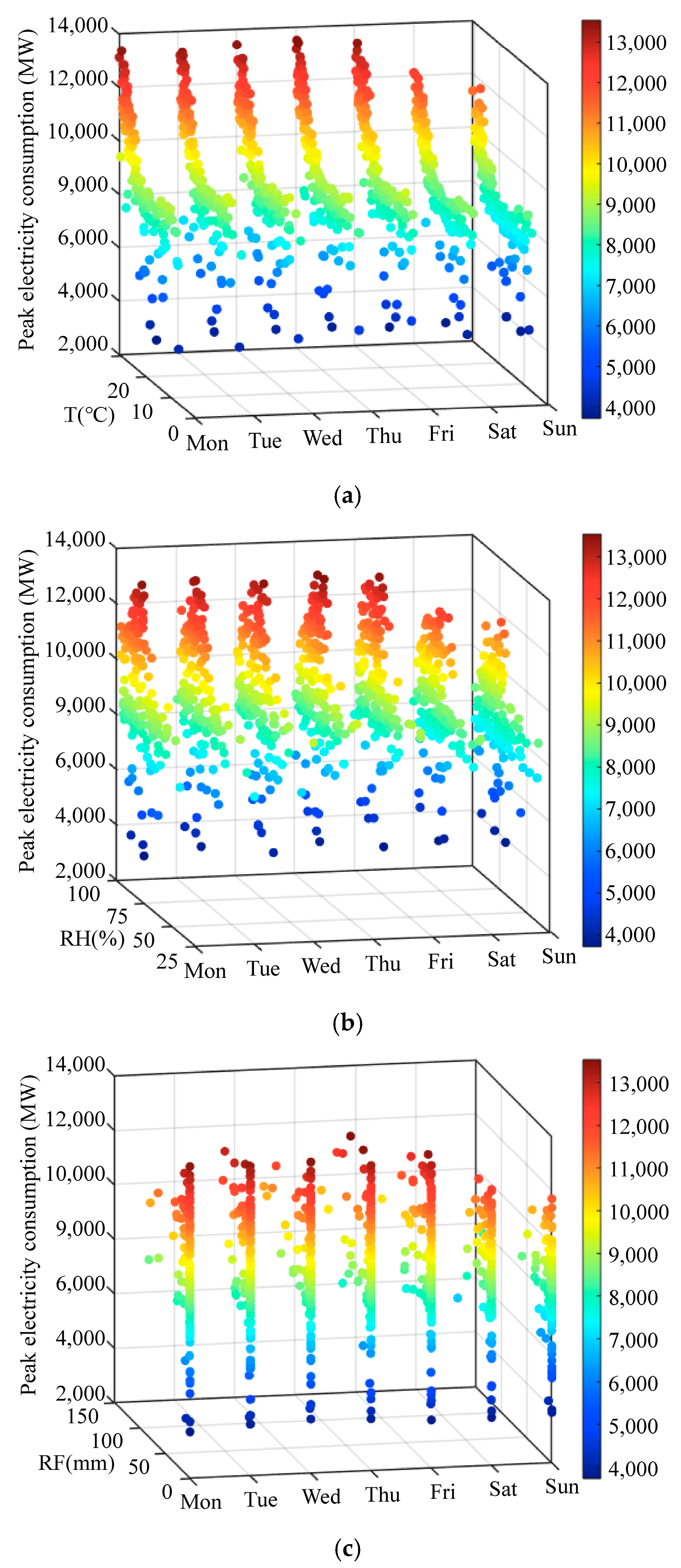
According to Figure 4, the maximum daily electricity consumption in this area gradually increases every year, and the daily peak load pattern is an inverted U shape. This is because in the modern power system, there are many types of electrical appliances that constitute the power load, and the proportion of loads affected by weather conditions such as air conditioners continues to increase, which increases the volatility and randomness of load changes. Figure 5 shows the spatial distribution of daily peak loads and their respective meteorological factors in this region.

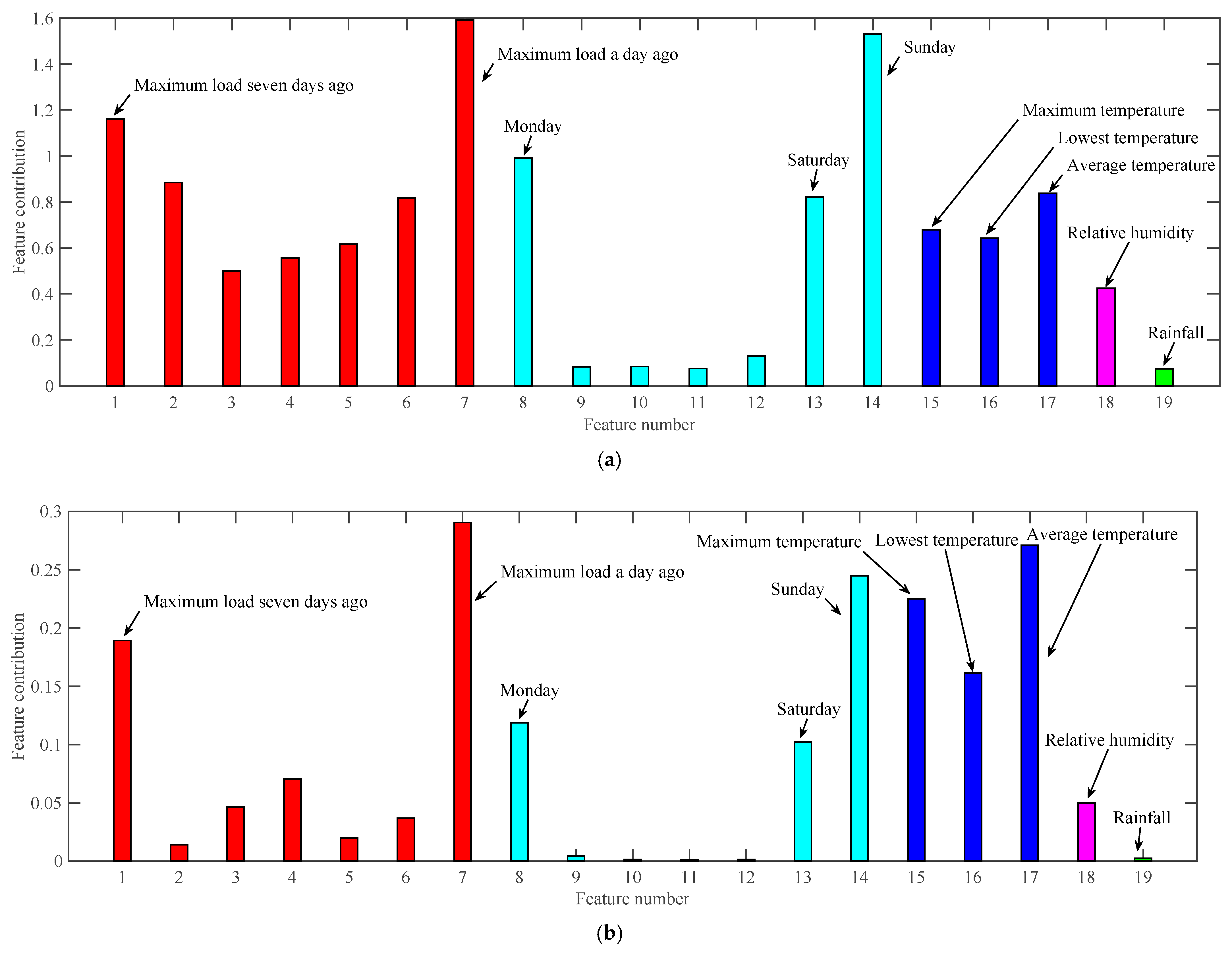
As shown in Figure 5, the load patterns on Saturdays and Sundays differ significantly from those observed on weekdays (Monday to Friday). Additionally, the daily maximum electricity consumption is strongly influenced by temperature fluctuations. Among the meteorological factors, although the effect of relative humidity on maximum power consumption is less pronounced than that of temperature, there is a discernible trend: as relative humidity increases, the daily maximum power consumption also tends to rise. Although rainfall is relatively frequent in this region, it has no significant impact on the maximum daily electricity consumption. Figure 6 presents the analysis of input feature contributions.

From the feature contribution scores of XGBoost and RF shown in Figure 6, it is evident that among the meteorological factors, rainfall has minimal impact on the daily maximum load during the forecast period. As a result, the effect of rainfall is excluded from the analysis. The input features for the period from Tuesday to Friday are combined into a single feature, and the meteorological input features include daily maximum temperature, minimum temperature, average temperature, and relative humidity.

While some studies have suggested a correlation between precipitation and power load, it was not included as a significant feature in this research. This decision is primarily due to the specific conditions of our study area—Western Inner Mongolia—where precipitation is frequent yet highly variable, having little direct impact on load, especially in short-term forecasts. Moreover, precipitation often works in tandem with temperature and humidity, occasionally influencing the use of air conditioning and heating systems, which in turn can affect load. However, in this study, temperature (particularly maximum temperature) and humidity were found to play a more substantial role in forecasting power load. As a result, we chose to exclude precipitation from the model, aiming to streamline the analysis, minimize potential noise, and ensure that the focus remains on the most influential meteorological variables for accurate predictions.

4.3. Sequence ICEEMDAN Decomposition

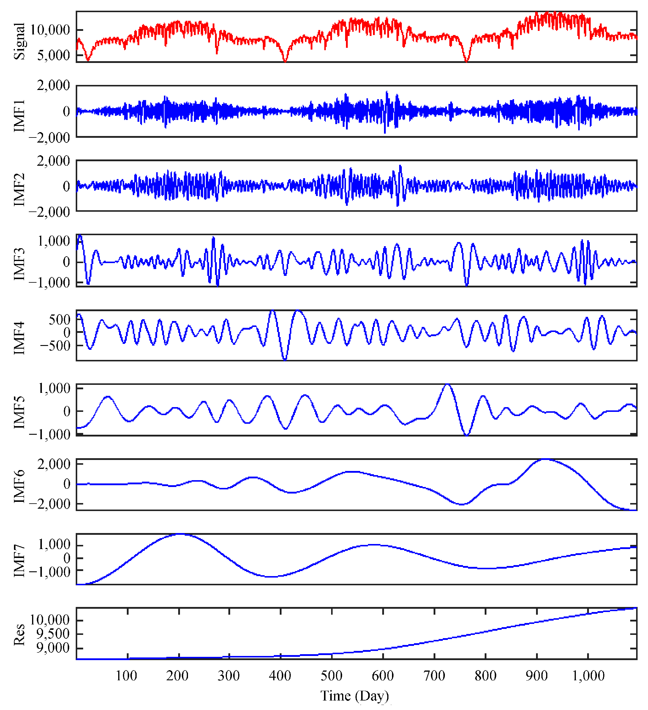
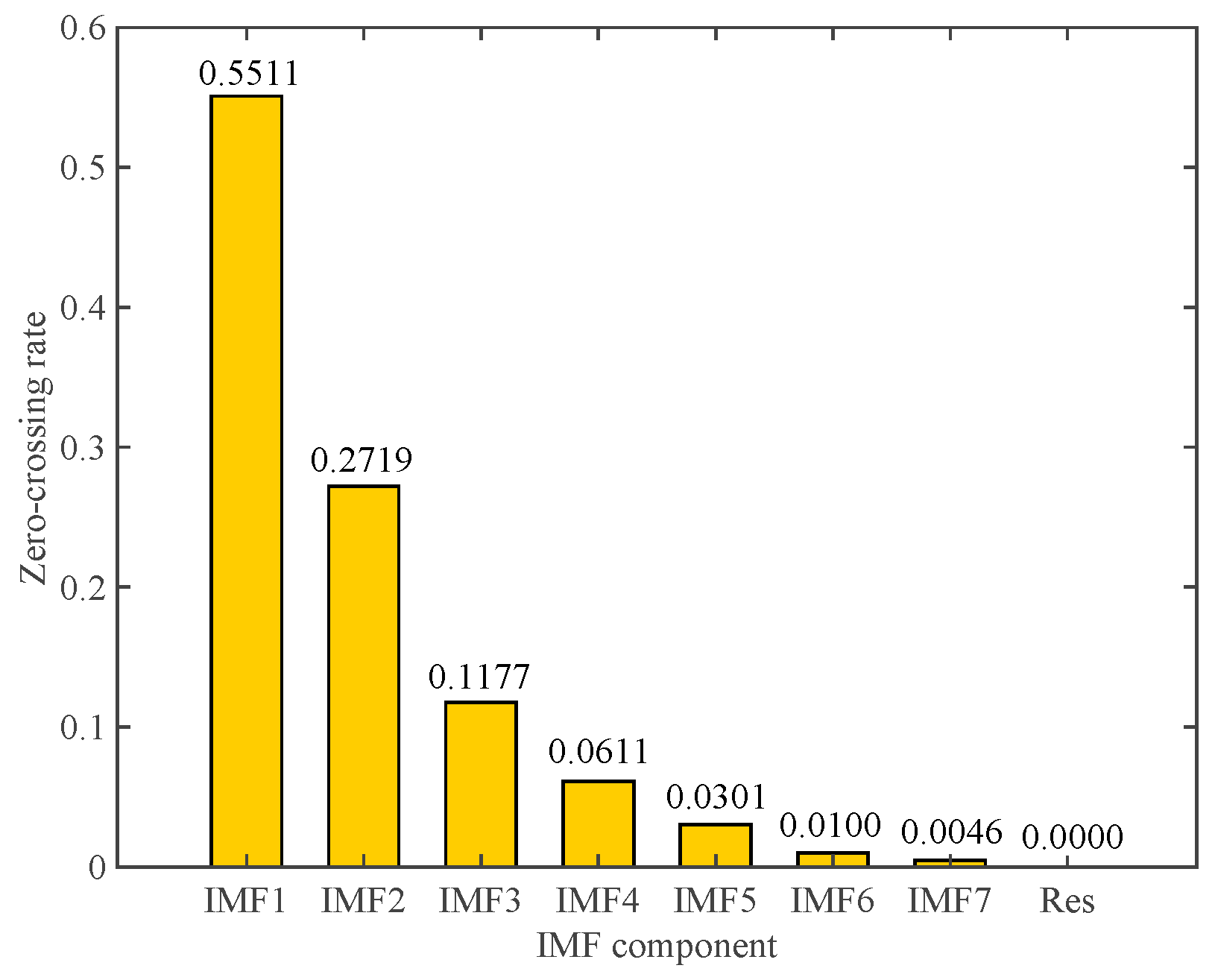
Figure 7 presents the decomposition results of ICEEMDAN applied to the daily peak load sequence. The zero-crossing rate of each IMF component obtained through ICEEMDAN decomposition is calculated, as shown in Figure 8. Based on the zero-crossing rates of the IMF components, high-frequency and stationary components are classified. Specifically, IMF1 to IMF3 are combined to form a new high-frequency component, IMF1′; IMF4 and IMF5 are combined into another high-frequency component, IMF2′; and IMF6 is included in a new high-frequency component, IMF2′. The remaining components are merged into a new stationary component, IMF3′. The high-frequency components, IMF1′ and IMF2′, are predicted using SSA-Bagging-XGBoost, while the stationary component, IMF3′, is predicted using MLR.

4.4. Hyperparameter Search Process

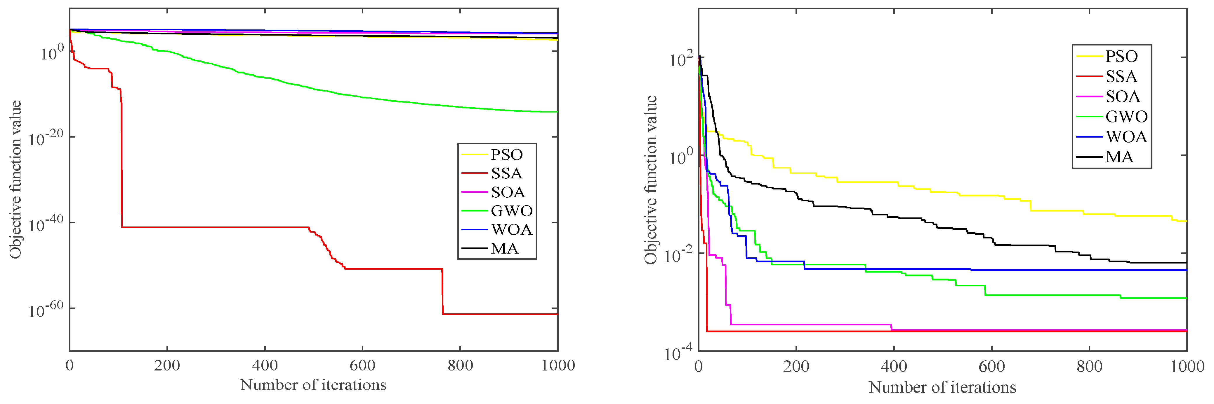
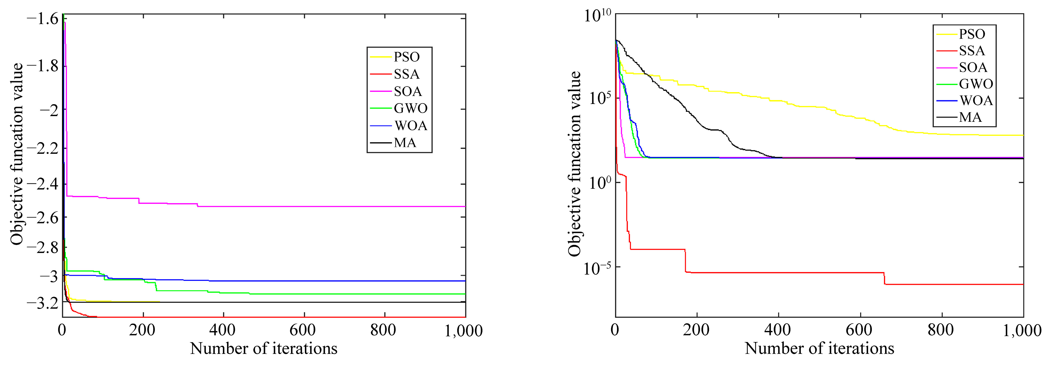
In this paper, the SSA is selected to optimize the hyperparameters of XGBoost. As shown in Figure 9, SSA demonstrates significant advantages in both convergence speed and global optimization capability. Experimental results indicate that SSA converges rapidly over multiple iterations and effectively avoids the issue of local optima, making it particularly effective for solving complex, high-dimensional, and multi-modal optimization problems. Compared to PSO, SSA is able to escape local optima during later iterations, ensuring a more thorough exploration of the global optimum. In comparison to GWO and WOA, SSA exhibits faster convergence and greater stability in multi-objective optimization problems. Moreover, when compared to MFO, SSA shows superior search efficiency and global optimization capability. In conclusion, the use of SSA for hyperparameter tuning of XGBoost in this study can significantly enhance the model’s predictive performance.

4.5. Comparative Analysis of Prediction Models

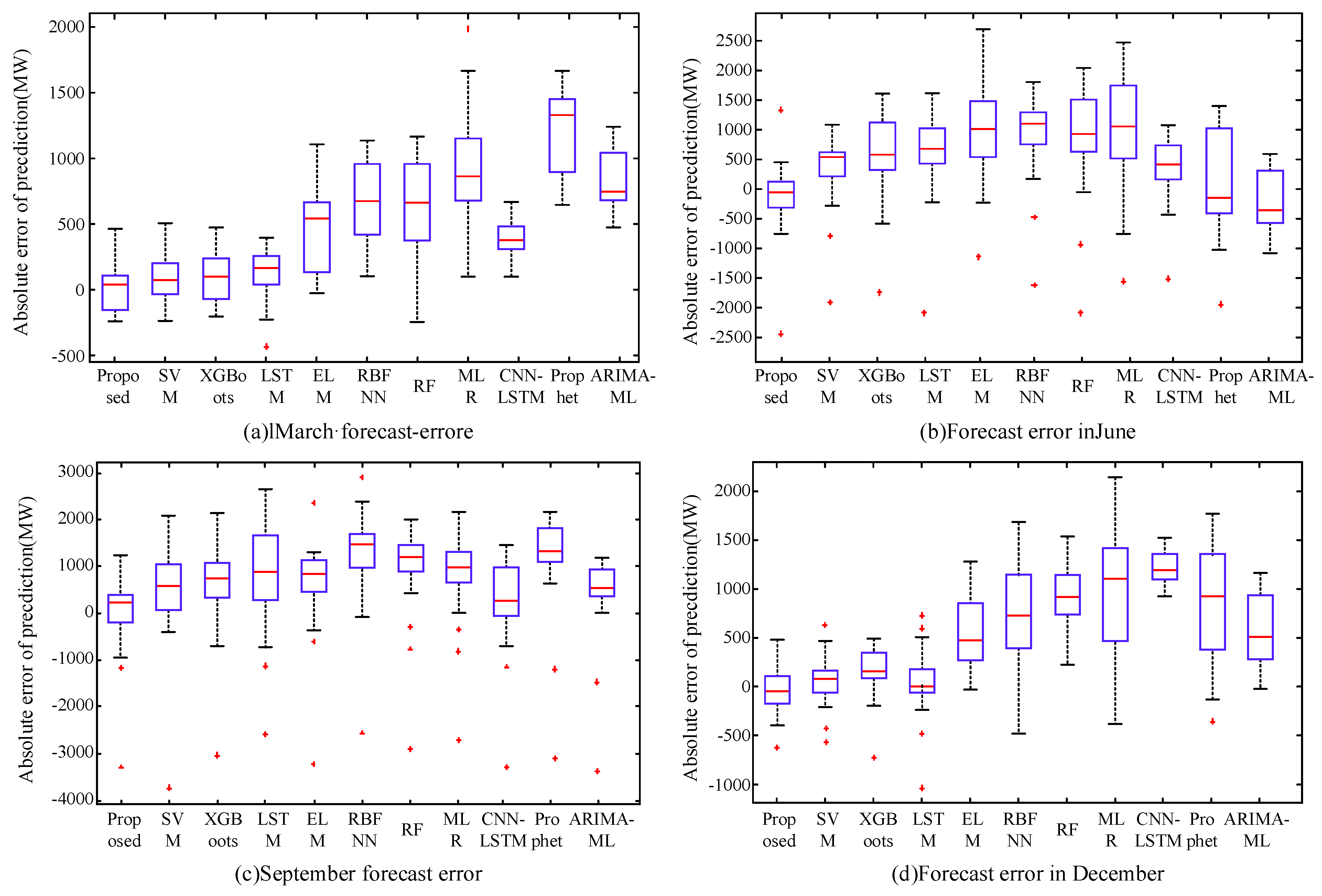
To validate the predictive performance of the ICEEMDAN-Bagging-XGBoost-MLR model proposed in this study, a comparison is made with both ensemble and single models. The model types and their corresponding prediction results are presented in Figure 10 and

Table 2. Comparison of prediction errors of each algorithm.

Algorithm	Indicators	March	June	September	December
	$e_{RMSE}\left(MW\right)$	177.15	576.27	817.91	263.61
Proposed	$e_{MAE}\left(MW\right)$	141.84	361.58	547.97	193.36
	$e_{MAPE}\left(\%\right)$	1.65	3.31	5.13	2.23
	$e_{RMSE}\left(MW\right)$	207.17	920.11	1137.34	296.93
XGBoost	$e_{MAE}\left(MW\right)$	173.76	773.18	942.41	241.15
	$e_{MAPE}\left(\%\right)$	1.99	6.47	8.23	2.75
	$e_{RMSE}\left(MW\right)$	731.85	1167.39	1303.76	1021.70
RF	$e_{MAE}\left(MW\right)$	666.01	1032.67	1198.35	940.47
	$e_{MAPE}\left(\%\right)$	7.55	8.66	10.38	10.54
	$e_{RMSE}\left(MW\right)$	182.65	732.98	1041.73	241.24
SVM	$e_{MAE}\left(MW\right)$	139.56	575.15	769.36	174.64
	$e_{MAPE}\left(\%\right)$	1.60	5.02	6.85	1.99
	$e_{RMSE}\left(MW\right)$	220.55	922.71	1317.93	316.98
LSTM	$e_{MAE}\left(MW\right)$	190.11	800.63	1090.02	202.57
	$e_{MAPE}\left(\%\right)$	2.20	6.82	9.40	2.30
	$e_{RMSE}\left(MW\right)$	716.19	1205.61	1603.76	886.89
RBFNN	$e_{MAE}\left(MW\right)$	658.71	1120.36	1463.08	781.68
	$e_{MAPE}\left(\%\right)$	7.48	9.59	12.58	8.80
	$e_{RMSE}\left(MW\right)$	529.59	1262.32	1123.58	668.41
ELM	$e_{MAE}\left(MW\right)$	430.84	1113.24	934.17	570.69
	$e_{MAPE}\left(\%\right)$	4.86	9.37	8.20	6.43
CNN-LSTM	$e_{RMSE}\left(MW\right)$	205.16	836.25	1003.27	289.24
	$e_{MAE}\left(MW\right)$	177.77	739.46	830.53	221.85
	$e_{MAPE}\left(\%\right)$	1.84	2.35	3.27	2.64
Prophet	$e_{RMSE}\left(MW\right)$	1235.23	1835.26	1300.98	1653.01
	$e_{MAE}\left(MW\right)$	1039.9	1644.27	1124.42	1265.07
	$e_{MAPE}\left(\%\right)$	15.81	18.41	11.26	15.28
ARIMA-ML	$e_{RMSE}\left(MW\right)$	976.53	1022.18	989.36	1021.02
	$e_{MAE}\left(MW\right)$	836.66	898.4	749.1	815.38
	$e_{MAPE}\left(\%\right)$	9.53	9.82	9.66	9.91
	$e_{RMSE}\left(MW\right)$	1039.51	1377.68	1222.65	1158.14
MLR	$e_{MAE}\left(MW\right)$	950.33	1194.96	1089.15	1015.69
	$e_{MAPE}\left(\%\right)$	10.95	9.92	9.41	11.49

. It is worth noting that, given the significant seasonal variations in load patterns, peak load predictions for March, June, September, and December are selected for comparison.

As illustrated in Figure 10 and Table 2, both SVM and LSTM demonstrate strong predictive accuracy when employed as single models in March and December. For instance, in March, SVM yields RMSE values of 177.15 MW, an MAE of 141.84 MW, and a MAPE of 1.65%. However, during June and September, the performance of SVM declines significantly, with RMSE values rising to 576.27 MW in June and 817.91 MW in September, the MAE reaching 361.58 MW and 547.97 MW, and the MAPE increasing to 3.31% and 5.13%, respectively. Similarly, LSTM exhibits favorable results for March and December but shows substantial error increases in June and September. In June, the RMSE is 920.11 MW, MAE is 773.18 MW, and MAPE is 6.47%; in September, these metrics rise to an RMSE of 1137.34 MW, MAE of 942.41 MW, and MAPE of 8.23%. These findings clearly indicate that the accuracy of single models deteriorates significantly when faced with months characterized by high data fluctuations.

Although the XGBoost ensemble model performs well in March and December, its accuracy in June and September remains markedly lower compared to that in other months. For example, in June, the RMSE is 1167.39 MW, MAE is 1032.67 MW, and MAPE is 8.66%, with even higher values in September—the RMSE reaches 1303.76 MW, the MAE reaches 1198.35 MW, and the MAPE reaches 10.38%. This indicates that XGBoost struggles to effectively handle data disturbances, leading to instability in its performance during months with high volatility.

The Prophet and MLR models, both based on linear regression, also fail to adequately address the complex and nonlinear relationships within the data. For instance, Prophet produces RMSE values of 1235.23 MW, MAE of 1039.90 MW, and MAPE of 15.81% in March. In June, the RMSE increases to 1835.26 MW, MAE to 1644.27 MW, and MAPE to 18.41%; and in September, these values reach RMSE of 1300.98 MW, MAE of 1124.42 MW, and MAPE of 11.26%. These results highlight the limitations of Prophet in capturing data volatility, with its linear assumptions unable to account for the nonlinearities in the data, leading to suboptimal predictive performance. Similarly, the MLR model fails to provide satisfactory results. In March, RMSE is 1039.51 MW, MAE is 950.33 MW, and MAPE is 10.95%; in June, RMSE is 1377.68 MW, MAE is 1194.96 MW, and MAPE is 9.92%; in September, RMSE is 1222.65 MW, MAE is 1089.15 MW, and MAPE is 9.41%; and in December, RMSE is 1158.14 MW, MAE is 1015.69 MW, and MAPE is 11.49%. These results suggest that MLR is unable to capture the nonlinear features of the data, leading to significant prediction errors.

In contrast, the proposed model demonstrates consistently high accuracy across all months, particularly in June and September, when the data exhibits significant volatility. Notably, when compared to Prophet and MLR, the proposed model shows a marked improvement in prediction accuracy during June. In Prophet, the RMSE is 1835.26 MW, MAE is 1644.27 MW, and MAPE is 18.41%; in MLR, the RMSE is 1377.68 MW, MAE is 1194.96 MW, and MAPE is 9.92%. In contrast, the proposed model achieves RMSE values of 836.25 MW, MAE of 739.46 MW, and MAPE of 2.35%. Specifically, the RMSE of the proposed model is reduced by 54.4% compared to Prophet and by 39.3% compared to MLR. Meanwhile, the MAPE is reduced by 87.3% compared to Prophet and by 76.3% compared to MLR. These results clearly demonstrate that the proposed model is capable of mitigating the impact of data disturbances, maintaining high prediction accuracy in volatile months, and showcasing its significant advantage in handling complex and fluctuating data.

4.6. Scalability Verification

Building on the previous research, we initially used data from a specific region in Western Inner Mongolia. However, we recognize that these data may not fully capture the range of peak load patterns found in other areas with varying climate conditions, infrastructure, and load characteristics. To strengthen the validation of our model, we expanded the scope of our analysis by including load data from a city in Northern China and its affiliated county-level State Grid Corporation. This dataset encompasses the total load data from over 30 key users, covering a period of three years, from 25 November 2020, to 25 November 2023, with daily load measurements throughout. Consistent with the previous sections, the data format, model training parameters, and comparison models are retained. The focus of the model’s prediction is the peak load for October 2023, with the results summarized in

Table 3. Comparison of prediction errors of each algorithm.

Algorithm	${\mathit{e}}_{\mathit{R}\mathit{M}\mathit{S}\mathit{E}}\left(\mathit{M}\mathit{W}\right)$	${\mathit{e}}_{\mathit{M}\mathit{A}\mathit{E}}\left(\mathit{M}\mathit{W}\right)$	${\mathit{e}}_{\mathit{M}\mathit{A}\mathit{P}\mathit{E}}\left(\mathbf{\%}\right)$
Proposed	11.44	9.47	1.28
RF	34.64	28.91	3.79
XGBoost	35.82	32.90	4.35
SVM	22.31	18.93	2.48
LSTM	21.59	17.80	2.40
RBFNN	37.11	32.96	4.34
ELM	25.18	21.50	2.94
CNN-LSTM	20.18	17.23	2.36
Prophet	32.58	27.02	4.21
ARIMA-ML	28.38	24.07	3.26
MLR	30.67	23.49	3.99

.

As presented in Table 3, the proposed model consistently outperforms all comparison models across key error metrics, including RMSE, MAE, and MAPE. With an RMSE of 11.44 MW, MAE of 9.47 MW, and MAPE of just 1.28%, the proposed model demonstrates its exceptional ability to predict peak loads with a high degree of accuracy, even when confronted with the intricate dynamics of regional load behaviors. In contrast, models like RF and XGBoost, though robust, show higher prediction errors. RF results in an RMSE of 34.64 MW, MAE of 28.91 MW, and MAPE of 3.79%, while XGBoost produces even higher errors, with an RMSE of 35.82 MW, MAE of 32.90 MW, and MAPE of 4.35%. These figures suggest that while ensemble models are typically effective, they struggle to capture peak load dynamics as effectively as the proposed model in this particular case. Similarly, SVM and LSTM perform reasonably well but still fall short compared to the proposed model. SVM achieves an RMSE of 22.31 MW, MAE of 18.93 MW, and MAPE of 2.48%, while LSTM records an RMSE of 21.59 MW, MAE of 17.80 MW, and MAPE of 2.40%. While these models offer solid performance, they do not reach the level of accuracy demonstrated by the proposed model, particularly in capturing peak load fluctuations.

The RBFNN and ELM models, though competitive, also yield higher errors, with RBFNN showing an RMSE of 37.11 MW and ELM an RMSE of 25.18 MW. Although CNN-LSTM brings a hybrid approach similar to LSTM, it still lags behind, achieving a MAPE of 2.36%, showing that traditional and hybrid models, while useful, do not match the performance of the proposed model in this context. Models based on time-series forecasting, such as Prophet and ARIMA-ML, also exhibit notable shortcomings. Prophet produces an RMSE of 32.58 MW, MAE of 27.02 MW, and MAPE of 4.21%, while ARIMA-ML shows an RMSE of 28.38 MW, MAE of 24.07 MW, and MAPE of 3.26%. These higher errors highlight the difficulty of time-series models in accurately predicting peak load events in this specific case.

In conclusion, the superior performance of the proposed model can be attributed to its hybrid structure, which effectively integrates the strengths of different algorithms while overcoming the limitations of individual models. The results solidify the proposed approach as a highly effective tool for peak load forecasting, demonstrating its reliability and robustness in managing complex, fluctuating load data.

5. Conclusions

This paper proposes a continuous multi-day peak load prediction model based on ICEEMDAN-Bagging-XGBoost-MLR and incorporates the SSA optimization algorithm to identify the optimal hyperparameters of XGBoost, thus reducing the time required for hyperparameter optimization. In the absence of temperature data for the upcoming month, the proposed model is applied to decompose the temperature series, retaining only the trend component that reflects the overall temperature changes, while discarding components with higher complexity and frequencies of variation. The analysis shows that the smoothed temperature series exhibits higher feature contribution scores, indicating that the overall temperature trend is the primary factor driving daily peak load variations, while the random fluctuations in temperature contribute less to these changes. The smoothing process employed is both logical and highly practical, demonstrating its applicability in similar forecasting scenarios. In addition, the proposed model effectively captures and tracks load variations, even during periods of significant fluctuations. When compared to both the ensemble and individual benchmark models, the proposed model consistently exhibits high and stable prediction accuracy across all months of the year, along with strong resistance to overfitting and impressive generalization capabilities. Of particular note is the fact that the RMSE of the proposed model is reduced by 54.4% compared to that of the Prophet model and by 39.3% compared to that of the MLR model. Additionally, the MAPE shows significant reductions of 87.3% and 76.3%, respectively, relative to that of Prophet and MLR. In further scalability assessment, the proposed model also outperformed all benchmark models, demonstrating its robustness.

The current model primarily focuses on daily peak load forecasting, which is highly effective for short-term predictions but may not yield satisfactory results for long-term forecasting. Incorporating external factors, such as seasonal variations, socio-economic changes, and infrastructure development, in future work could extend the model’s applicability to longer-term forecasts.

References

1. Gao, Y.; Tahir, M.; Siano, P.; Bi, Y.; Hu, S.; Yang, J. Optimization of renewable energy-based integrated energy systems: A three-stage stochastic robust model. Appl. Energy 2025, 377, 124635. [Google Scholar] [CrossRef]
2. Meng, Q.; Jin, X.; Luo, F.; Wang, Z.; Hussain, S. Distributionally robust scheduling for benefit allocation in regional integrated energy system with multiple stakeholders. J. Mod. Power Syst. Clean Energy 2024, 12, 1631–1642. [Google Scholar] [CrossRef]
3. Wood, M.; Matrone, S.; Ogliari, E.; Leva, S. Comparing peak electricity load forecasting models for an industrial and a residential building. Math. Comput. Simul. 2026, 240, 303–316. [Google Scholar] [CrossRef]
4. Gao, Y.; Zhao, Y.; Hu, S.; Tahir, M.; Yuan, W.; Yang, J. A three-stage adjustable robust optimization framework for energy base leveraging transfer learning. Energy 2025, 319, 135037. [Google Scholar] [CrossRef]
5. Hong, Y.Y.; Apolinario, G.F.D.G.; Cheng, Y.H. Week-ahead daily peak load forecasting using hybrid convolutional neural network. IFAC PapersOnLine 2023, 56, 372–377. [Google Scholar] [CrossRef]
6. Gao, Z.; Yin, X.; Zhao, F.; Meng, H.; Hao, Y.; Yu, M. A two-layer SSA-XGBoost-MLR continuous multi-day peak load forecasting method based on hybrid aggregated two-phase decomposition. Energy Rep. 2022, 8, 12426–12441. [Google Scholar] [CrossRef]
7. Lianbing, L.I.; Guoqiang, G.A.; Weiguang, C.H.; Wenjie, F.U.; Chao, Z.H.; Shasha, Z.H. Ultra short term load power prediction considering feature recombination and BiGRU-Attention-XGBoost model. Mod. Electr. Power 2023, 41, 1–11. [Google Scholar]
8. Cai, Q.; Chao, Z.; Su, B.; Wang, L.; Duan, Q.; Wen, Y.; Li, B. Short-term load forecasting method based on a novel robust loss neural network algorithm. Power Syst. Technol. 2020, 44, 4132–4139. [Google Scholar]
9. Yu, Y.-L.; Li, W.; Sheng, D.-R.; Chen, J.-H. A hybrid short-term load forecasting method based on improved ensemble empirical mode decomposition and back propagation neural network. J. Zhejiang Univ. Sci. A Appl. Phys. Eng. 2016, 17, 101–114. [Google Scholar] [CrossRef]
10. Pang, H.; Gao, J.; Du, Y. A short-term load probability density prediction based on quantile regression of time convolution network. Power Syst. Technol. 2020, 44, 1343–1350. [Google Scholar]
11. Fan, S.; Li, L.; Wang, S.; Liu, X.; Yu, Y.; Hao, B. Application analysis and exploration of artificial intelligence technology in power grid dispatch and control. Power Syst. Technol. 2020, 44, 401–411. [Google Scholar]
12. Wang, S.; Wang, X.; Wang, S.; Wang, D. Bi-directional long short-term memory method based on attention mechanism and rolling update for short-term load forecasting. Int. J. Electr. Power Energy Syst. 2019, 109, 470–479. [Google Scholar] [CrossRef]
13. Chang, Y.; Sun, H.; Gu, T.; Du, W.; Wang, Y.; Li, W. Monthly forecast of wind power generation using historical data expansion method. Power Syst. Technol. 2021, 45, 1059–1068. [Google Scholar]
14. Xu, Y.; Xiang, Y.; Ma, T. VMD-GRU short-term power load forecasting model based on optimized parameters of particle swarm algorithm. J. North China Electr. Power Univ. (Nat. Sci. Ed.) 2023, 50, 38–47. [Google Scholar]
15. Li, Y.; Liu, X.; Xing, F.; Wen, G.; Lu, N.; He, H.; Jiao, R. Daily peak load prediction based on correlation analysis and bi-directional long short-term memory network. Power Syst. Technol. 2021, 45, 2719–2730. [Google Scholar]
16. Rafi, S.H.; Al-Masood, N.; Deeba, S.R.; Hossain, E. A short-term load forecasting method using integrated CNN and LSTM network. IEEE Access 2021, 9, 32436–32448. [Google Scholar] [CrossRef]
17. Tang, X.; Dai, Y.; Liu, Q.; Dang, X.; Xu, J. Application of bidirectional recurrent neural network combined with deep belief network in short-term load forecasting. IEEE Access 2019, 7, 160660–160670. [Google Scholar] [CrossRef]
18. Afrasiabi, M.; Mohammadi, M.; Rastegar, M.; Stankovic, L.; Afrasiabi, S.; Khazaei, M. Deep-based conditional probability density function forecasting of residential loads. IEEE Trans. Smart Grid 2020, 11, 3646–3657. [Google Scholar] [CrossRef]
19. Al-Rakhami, M.; Gumaei, A.; Alsanad, A.; Alamri, A.; Hassan, M.M. An ensemble learning approach for accurate energy load prediction in residential buildings. IEEE Access 2019, 7, 48328–48338. [Google Scholar] [CrossRef]
20. Shi, J.; Ma, L.; Li, C.; Liu, N.; Zhang, J. Peak load forecasting method based on serial-parallel ensemble learning. Chin. J. Electr. Eng. 2020, 40, 4463–4472, 4726. [Google Scholar]
21. Yu, Y.; Wang, Z.; Chen, X.; Feng, Q. Particle swarm optimization algorithm based on teaming behavior. Knowl. Based Syst. 2025, 318, 113555. [Google Scholar] [CrossRef]
22. Jin, Z.; Li, X.; Qiu, Z.; Li, F.; Kong, E.; Li, B. A data-driven framework for lithium-ion battery RUL using LSTM and XGBoost with feature selection via Binary Firefly Algorithm. Energy 2025, 314, 134229. [Google Scholar] [CrossRef]
23. Wang, L.; Peng, L.; Xiong, X.; Li, Y.; Qi, Y.; Hu, X. Research on high-speed constant tension spinning control strategy based on vibration detection and enhanced firefly algorithm based FOPID controller. Measurement 2025, 117, 117789. [Google Scholar] [CrossRef]
24. Meng, Q.; Xu, J.; Ge, L.; Wang, Z.; Wang, J.; Xu, L.; Tang, Z. Economic optimization operation approach of integrated energy system considering wind power consumption and flexible load regulation. J. Electr. Eng. Technol. 2024, 19, 209–221. [Google Scholar] [CrossRef]
25. Meng, Q.; Zu, G.; Ge, L.; Li, S.; Xu, L.; Wang, R.; He, K.; Jin, S. Dispatching strategy for low-carbon flexible operation of park-level integrated energy system. Appl. Sci. 2022, 12, 12309. [Google Scholar] [CrossRef]
26. Liang, B.; Feng, W. Bearing fault diagnosis based on ICEEMDAN deep learning network. Processes 2023, 11, 2440. [Google Scholar] [CrossRef]
Figure 1. ICEEMDAN-Bagging-XGBoost-MLR double-layer peak load forecasting model framework.
Applsci 15 11180 g001
Figure 2. XGBoost algorithm mechanism.
Applsci 15 11180 g002
Figure 3. Bagging parallel ensemble learning architecture.
Applsci 15 11180 g003
Figure 4. Original peak load sequence.
Applsci 15 11180 g004
Figure 5. Spatial distribution of peak load historical data. (a) Historical data of daily peak load and spatial distribution of average temperature. (b) Historical data of daily peak load and spatial distribution of relative humidity. (c) Historical data of daily peak load and spatial distribution of rainfall.
Applsci 15 11180 g005
Figure 6. Input feature contribution analysis. (a) RF feature contribution analysis. (b) XGBoost feature contribution analysis.
Applsci 15 11180 g006
Figure 7. ICCEMDAN decomposition results.
Applsci 15 11180 g007
Figure 8. Zero-crossing rate of each IMF component.
Applsci 15 11180 g008
Figure 9. Test results of different group optimization algorithms.
Applsci 15 11180 g009aApplsci 15 11180 g009b
Figure 10. The absolute error of each model prediction.
Applsci 15 11180 g010