A Dynamic Multi-Objective Optimization Algorithm for AGV Routing in Assembly Workshops

Abstract

This study tackles the complex challenge of dynamic multi-objective vehicle routing optimization in large-scale equipment manufacturing, where routing operations significantly impact both economic performance and environmental sustainability. We develop an innovative Dynamic Multi-Objective Vehicle Routing Problem (DMOVRP) model that uniquely integrates three competing objectives: environmental impact reduction, delivery timeliness, and operational robustness. The proposed algorithm combines a dynamic event handler with the NSACOWDRL algorithm—an adaptive multi-objective optimization algorithm with dynamic event handling capability. The proposed system features adaptive mechanisms for handling real-time disruptions through specialized event classification and dynamic rescheduling protocols. Extensive computational experiments demonstrate the algorithm’s superior performance with statistically significant improvements using the Wilcoxon signed-rank test (p < 0.05, n = 30 runs per instance), achieving average relative gains of 15.2% in HV, 12.8% in IGD, and 8.9% in GD metrics compared to established methods. This research makes theoretical contributions through its feasibility quantification metric and practical advancements in routing schedule systems. By successfully reconciling traditionally conflicting objectives through dynamic JIT adjustments and robustness-aware optimization, this work provides manufacturers with a versatile decision-support tool that adapts to unpredictable workshop conditions while maintaining sustainable operations.

1. Introduction

The integration of global supply chains has rendered logistics optimization a critical determinant of manufacturing competitiveness. However, transportation costs constitute a substantial expenditure component, representing 18–32% of total operational expenses in manufacturing sectors. Notably, vehicle routing processes contribute upwards of 40% of logistics-related energy consumption and carbon emissions. This dual imperative of economic efficiency and environmental sustainability necessitates advanced intelligent routing solutions capable of simultaneously optimizing costs while minimizing carbon footprint.

Vehicle routing optimization in large-scale equipment manufacturing facilities, considering significant spatial and temporal constraints, constitutes a variant of the Vehicle Routing Problem (VRP) [1]. The VRP aims to identify optimal routes under specified constraints and objectives and finds broad application in domains such as traffic management and logistics transportation. To better reflect practical logistics operations, several VRP variants have been developed, including the Dynamic VRP (DVRP) and the Multi-Objective VRP (MOVRP). Numerous researchers have conducted systematic literature reviews on these problems.

The dynamic vehicle routing problem (DVRP) addresses the stochastic nature inherent in real-world VRP variants [2]. In DVRP formulations, at least one problem parameter evolves temporally. Such dynamics may impact constraints, objective functions, customer demands, or vehicle workloads. Regarding multi-objective vehicle routing problems, Zajac et al. [3] provide a comprehensive review categorizing application-oriented MOVRPs by planning hierarchy and analyzing the nature of investigated trade-offs.

Although numerous methods have been proposed to address DVRP and MOVRP models, existing dynamic models are often limited to single-objective optimization, which significantly deviates from real-world requirements. Meanwhile, static multi-objective models frequently exhibit inadequate capability in handling dynamic anomalies commonly encountered in large-scale equipment manufacturing. To overcome these limitations, this study proposes integrating DVRP and MOVRP frameworks to establish a novel DMOVRP (Dynamic Multi-Objective Vehicle Routing Problem) model.

Studying DMOVRP is further motivated by its strong relevance to real-world applications, particularly in modern logistics. While prior research has extensively modeled mobile robots for automating repetitive and physically demanding tasks in VRP frameworks (e.g., N. Vimal Kumar et al. [4]), DMOVRP offers a broader methodological framework and enhanced robustness for addressing contemporary logistics challenges. Given the shared mathematical foundations between both problem classes—characterized by vehicles departing from and returning to a central depot, servicing customer demands under time constraints, and optimizing multiple objectives subject to capacity limitations—this study follows the methodology established by Pouya Baniasadi et al. [5] by developing algorithms that reformulate complex logistics scenarios into classical VRP constructs.

To address these challenges, this paper proposes a hybrid “static + dynamic” dual-scheduling model by extending the framework of static models to incorporate dynamic anomaly production and handling. A dynamic multi-objective optimization algorithm is specifically designed to solve the proposed model. To sum up, the main contributions of this paper are as follows:

(1) A dynamic multi-objective optimization formulation was developed for large-scale equipment manufacturing, simultaneously addressing carbon emissions, lead time, and infeasibility minimization. The model integrates spatiotemporal constraints for vehicle routing and demand fulfillment while accounting for transportation time uncertainty through stochastic coefficients. Solution robustness under uncertainty was quantified via a novel feasibility alpha metric. Robustness optimization was explicitly incorporated as an objective function to enhance solution reliability. The formulation reconciles conflicting Just-in-Time (JIT) scheduling and robustness objectives by implementing dynamic JIT deadlines instead of conventional time windows. A hybrid “dynamic exception handling-static optimization” framework was proposed to improve adaptability to stochastic operational disruptions.

(2) To address dynamic vehicle routing, a dynamic event handler and the NSACOWDRL (Non-dominated Sorting Ant Colony Optimization with Deep Reinforcement Learning) algorithm were proposed. The problem was decomposed into three stages:

1.

Multi-objective optimization (NSACOWDRL): A reference point-based niche preservation strategy ensured solution diversity. Pheromone updates incorporated non-dominated ranking and elite path reinforcement, while max–min pheromone bounds prevented premature convergence.

2.

Robustness selection: Monte Carlo simulations quantified solution feasibility, and uniform weight-based selection derived a diverse Pareto-optimal set.

3.

Dynamic re-optimization (DSACOWDEL): The event handler updated material demands, triggering adaptive rescheduling.

(3) Computational experiments across multi-scale instances with varying disruption intensities demonstrated NSACOWDRL superior performance in dynamic multi-objective optimization compared to MOEA/D and NSGA-III. Ablation studies verified the significant contribution of the embedded DDQN local search strategy.

The remainder of this paper is structured as follows: Section 2 presents essential background. Section 3 formulates the DMOVRP problem for assembly workshop logistics. Section 4 details the multi-objective, multi-stage dynamic routing methodology, including the NSACOWDRL algorithm and dynamic event handler. Experimental design and computational results are analyzed in Section 5. Finally, conclusions and suggestions for future work are outlined in Section 6.

2. Background

Since VRP is an NP-hard problem, finding optimal solutions is extremely challenging. As evident from the aforementioned research, the proposed VRP solution methods primarily aim to identify near-optimal solutions through efficient computational approaches. Common path planning problems for Automated Guided Vehicles (AGVs) are typically solved using exact algorithms and intelligent evolutionary algorithms.

Exact algorithms—including branch-and-bound, branch-and-price, integer linear programming, and cutting plane methods—are primarily applicable to small-scale VRP instances with simple structural configurations. Reihaneh et al. [6] developed a branch-price-and-cut algorithm for the Vehicle Routing Problem with Demand Allocation (VRPDA), while Tilk et al. [7] and Li et al. [8], respectively, addressed the Active-Passive Vehicle Routing Problem (APVRP) and a Synchronized Split-Delivery VRP with time windows and service-time constraints. Nevertheless, exact methodologies frequently exhibit limitations such as local optimum entrapment or computationally prohibitive runtime complexity for large-scale VRPs.

Several studies explore integrating exact methods with intelligent evolutionary algorithms. Kim et al. [9] developed a learning-based separation heuristic incorporating graph coarsening, which employs graph neural networks (GNNs) to approximate solutions for exact separation problems.

In contrast, intelligent evolutionary algorithms can find satisfactory near-optimal solutions for large-scale vehicle routing problems (VRPs) within limited computation time. As a result, intelligent optimization algorithms have become the mainstream approach for solving MOVRPs and DVRPs, and many researchers are devoted to improving and designing such algorithms.

Traditional single-objective VRP formulations and solution techniques inadequately address inherent multi-objective complexities, lacking the systemic perspective necessary for practical implementation. Consequently, multi-objective optimization problems (MOPs) are mathematically formulated to concurrently optimize conflicting objectives. As the predominant approach for MOP resolution, multi-objective evolutionary algorithms (MOEAs) have become the dominant methodology in this domain.

According to different algorithm strategies, most MOEAs can be classified into the following categories: (1) based on their dominant relationships, such as the NSGA-II [10], NSGA-III [11], SPEA [1], and PESA-II [12]; (2) based on decomposition, such as the MOEA/D [13], MOEA/DM2M [14], and RVEA [15]; (3) based on performance evaluation indicators, such as the IBEA [16], SMSEMOA [17], DNMOEA/HI [18], HypE [19], and FastHypervolume [20].

For DVRP methodologies, existing approaches employ discretized time windows, which is a paradigm introduced to manage dynamic scenarios. This framework partitions the operational horizon into equidistant intervals. A static optimization procedure is then iteratively executed for each interval to solve the corresponding routing subproblem. These methodologies are classified as periodic re-optimization techniques. Representative metaheuristic implementations for DVRP include greedy randomized adaptive search procedures [21], tabu search [22], ant colony optimization [21,23,24], genetic algorithms [22,25], memetic algorithms [26], monarch butterfly optimization [27], brainstorm optimization [28], and particle swarm optimization [29,30,31].

Beyond metaheuristic approaches, Large Neighborhood Search (LNS) and hybrid tabu–LNS methods have emerged as state-of-the-art techniques for the dynamic VRP. Pisinger and Røpke [32] demonstrated LNS’s effectiveness in real-time scenarios, while hybrid approaches combining tabu search with LNS [33] have shown superior performance in handling large-scale instances. These methods are particularly relevant for dynamic VRP comparisons, as they provide strong baselines for practical implementations.

Finally, recent research integrates optimization algorithms with machine learning to solve Vehicle Routing Problems (VRPs) effectively. Wang et al. [34] proposed Generative Inverse Reinforcement Learning (GIRL), combining adversarial networks with deep reinforcement learning to autonomously learn reward functions and 2-opt heuristics for routing optimization. Zhao et al. [35] introduced a hybrid framework using deep reinforcement learning (DRL) with an adaptive critic and local search, where the DRL generates initial solutions refined by classical heuristics like Large Neighborhood Search (LNS). Zhang et al. [36] designed a two-stage approach: imitation learning clones solutions from heuristic experts, followed by reinforcement learning to enhance policy exploration. Meanwhile, Ara et al. [37] applied reinforcement learning to optimize routes dynamically using environmental feedback. These approaches consistently outperform traditional methods in solution quality and computational speed for large-scale VRPs.

3. Problem Description and Mathematical Models

The assembly workshop AGV routing problem naturally maps to the Vehicle Routing Problem (VRP) framework. Both problems share the same fundamental structure: vehicles departing from a central depot (raw material warehouse) to serve distributed demand points (workstations) under capacity and time constraints. The AGVs function as delivery vehicles, workstation material demands correspond to customer demands, and Just-In-Time requirements align with time windows in VRPTW. This structural equivalence allows us to leverage established VRP solution methods while incorporating workshop-specific features through additional constraints such as robustness metrics and energy consumption objectives.

The escalating complexity of contemporary assembly workshop environments necessitates enhanced dynamic adaptability and real-time responsiveness in vehicle routing models. To address these challenges, we have extended our foundational static framework to develop a Dynamic Multi-Objective Vehicle Routing Problem.

3.1. Problem Description

For the convenience of explanation, Table 1 provides explanations of the model parameters and their corresponding variables.

Table 1. Model Parameter Setting.

Parameters	Meaning
V	Set of workstations,$V=\{0,1,\dots ,n\}$
$i,j$	Workstation nodes, $i,j\in V$. $i=0$ or $j=0$ corresponds to the raw material library
K	The total number of AGVs
R	The maximum number of material carriers that an AGV can transport
N	The total number of workstations in assembly workshop
M	The total number of material types
$[a_i,b_i]$	The time window at workstation i
T	The unit unloading time per material container
$d{y}_{Num}$	Dynamic events. When $Num=1$, dynamic work triggers a Class 1 dynamic event; when $Num=2$, dynamic work triggers a Class 2 dynamic.
$N_{d{y}_{Num}}$	The dynamic event $d{y}_{Num}$ triggered workstation
$Vo{l}_{N_{D{y}_{Num}}}$	The demand volume of dynamic event $Num$
$W_{N_{D{y}_{Num}}}$	The demand weight of dynamic event $Num$
${(X,Y)}_{N_{D{y}_{Num}}}$	The demand location of dynamic event $Num$
$[a_{N_{D{y}_{Num}}},b_{N_{D{y}_{Num}}}]$	The demand time window of dynamic event $Num$
$y_{ik}$	Whether workstation i is served by AGV k, where $y_{ik}=1$ if AGV k performs material delivery to workstation i, and $y_{ik}=0$ otherwise
$x_{ijk}$	Whether delivery mission between workstation i and workstation j is served by AGV k, where $x_{ijk}=1$ if AGV k performs material delivery from workstation i to workstation j, and $x_{ijk}=0$ otherwise
$R_k$	The material carriers quantity of the k-th AGV
$s_i$	Service time at i-th workstation
$q_i$	The unloading container quantity at workstation i
$[a_{ie},b_{ie}]$	The time window of the e-th material at workstation i
$JI{T}_i$	The due time for workstation i
p	Allowance rate
Q	The maximum capacity per vehicle
$t_j$	Arrival time of the AGV at station j
$t_i$	Arrival time of the AGV at station i
$d_{ij}$	The distance between station i and j
v	The speed of AGV
$t_i^{\sim }$	The uncertainty in the arrival time of the AGV at workstation i
$\widetilde{u_{ij}}$	The characteristic coefficient between stations i and j
$\overline{D}$	The average distance between workstations
$\zeta$	Global stochastic disturbances
$\overline{\zeta }$	Average stochastic disturbances
$interva{l}_{ij}^{\sim }$	The uncertainty in the transition from workstation i to workstation j
${\alpha }_{ij}$	The feasibility of the path from workstation j to workstation i
$w_{ie}$	The lead time of the e-th material for workstation i
$JI{T}_{ie}$	The due time of the e-th material for workstation i
$E_i$	All materials required for workstation i
$w_{kmin}$	The time delay of the k-th AGV departing from the warehouse
$N_k$	The set of workstations assigned to the k-th AGV
$E_k$	The total energy consumption of the k-th AGV
$E_{acc}^k$	The energy consumption of the k-th vehicle during acceleration and deceleration
$E_{cru}^k$	The energy consumption of the k-th vehicle during constant-speed travel
$q_{ie}$	The number of containers for the e-th material at workstation i
$b_{im}$	The weight of the m-th material required by workstation i
$Vo{l}_i$	The volume of the materials required by workstation i
$Vo{l}_{ie}$	The volume of the e-th material required by workstation i
$C_{ij}$	The energy consumed between workstation i and j
$C{L}_{ik}$	The remaining energy of AGV k at workstation i
$C_k$	The carbon emissions of the path of the k-th AGV
$C_{max}$	The carbon emission cap
$D_y$	Dynamic events list
$event$	The number of dynamic events
$T_{AGV}^K$	The departure time of AGV k
$T_{d{y}_{Num}}$	The dynamic workstation’s appearance time
$N_{AGV}$	The set of AGVs which satisfy the condition of $T_{AGV}^K>T_{d{y}_1}$
$i^{*}$	Updated workstation
$V\left(i^{*}\right)$	Workstation set composed of Workstation $i^{*}$
$V_k$	The set of workstations transported by AGV k
$W_k$	The AGV with minimum loading weight
$Q_k$	The AGV with minimum loading
$T^i$	The delivery time of the i-th workstation
$k^{*}$	The AGV number selected for rescheduling
$V_{k^{*}}$	The set of workstations assigned to AGV $k^{*}$

In this paper, the Dynamic Multi-Objectives Vehicle Routing Problem (DMOVRP) in assembly workshop environments is described as follows:

Let $i,j$ denote workstation nodes, where $i,j\in V$ and $V=\{0,1,\dots ,n\}$ represents the set of workstations. Here, $i=0$ or $j=0$ corresponds to the raw material library. The warehouse is equipped with K homogeneous automated guided vehicles (AGVs) with unlimited maximum travel distance.

Materials are transported via towed carts and each attached to an AGV’s rear hitch. Each AGV can carry a maximum of R carts. The assembly workshop consists of N workstations requiring M types of materials. Materials are categorized into:

1.

Small materials: High variety and quantity but small in size. Each type is consolidated into standardized containers and treated as a single unit.

2.

Large materials: Low variety but bulky, transported individually.

The workstation–material assignments are predefined, with all material information and workstation coordinates known.

The AGVs must deliver M materials to N workstations. Due to stochastic disturbances, transportation times are uncertain. Traditional time windows $[a_i,b_i]$ are replaced by Just-in-Time (JIT) deadlines $JI{T}_i$, requiring materials to arrive exactly before $JI{T}_i$.

At time T within each delivery cycle, stochastic dynamic events are triggered. These events are classified into two categories based on common workshop disruptions:

1.

Type I (Demand Cancellation): the material demand at workstation $N_{dy1}$ is canceled, and $N_{dy1}$ is removed from the demand list.

2.

Type II (New Demand Generation): a new demand arises at workstation $N_{dy2}$, requiring AGVs to deliver material $N_{dy2}$ with volume $Vo{l}_{N_{dy2}}$, weight $W_{N_{dy2}}$, and coordinates ${(X,Y)}_{N_{dy2}}$ within the time window $[a_{N_{dy2}},b_{N_{dy2}}]$.

When detecting dynamic events, the dynamic model updates the demand list and initiates AGV rescheduling. The system adapts to Type I/II events via real-time re-optimization to fulfill new demands while maintaining Just-in-Time (JIT) compliance.

The VRP problem in the assembly workshop is based on the following assumptions:

1.

The workshop has a centralized raw material library capable of fulfilling all workstation demands.

2.

The material demand at any workstation does not exceed the AGV’s load capacity.

3.

Unloading times at all workstations are deterministic and known a priori.

4.

All AGVs depart from and must return to the raw material library after completing deliveries.

5.

AGV dynamics and charging processes are neglected during operation.

6.

Materials are packed in standardized boxes and cannot be split for delivery.

7.

Each AGV tows material carts, with boxes for the same workstation consolidated into a single cart. Cross-workstation mixing of materials is prohibited.

8.

The fleet size remains constant throughout the planning horizon, with no additional vehicles generated during dynamic re-planning.

9.

Dynamic event demands never exceed the vehicle’s fixed constraints, including load capacity and volumetric limitations.

10.

Time delays between event occurrence and system reporting are negligible, enabling real-time event processing and immediate rescheduling.

11.

When Type II dynamic events occur, the corresponding workstation’s demand remains unfulfilled until the new schedule is executed.

3.2. Mathematic Model

3.2.1. Multi-Objective Model

The three objectives for the MODVRP can be stated as follows:

$f_{LC}$ (Low carbon):

$$min{f}_{LC}=\sum _{k=1}^K{E}_k$$

(1)

${\alpha }_i$ (Robustness metrics):

$$min{\alpha }_i={\displaystyle \frac{1}{{\prod }_{i=1}^N{\alpha }_i}}$$

(2)

$f_{JIT}$ (Penalty time):

$$min{f}_{JIT}=\sum _{k=1}^K{w}_k$$

(3)

f (Overall objectives):

$$minf=(f_{LC},{\alpha }_i,f_{JIT})$$

(4)

The constraints associated with the DMOVRP are added as follows:

1. Material vehicle quantity constraints: The number of material vehicles at each AGV delivery station should not exceed its own material vehicle capacity. The material vehicle quantity for each AGV cannot surpass the AGV’s maximum material vehicle capacity.

$$\sum _{i=0}^N{y}_{ik}\le R_k\le R,(k=1,2,\dots ,m)$$

(5)

2. Service time $s_i$:

The workstation service time is a function of the quantity of material containers scheduled for delivery.

$$s_i=\left\{\begin{array}{cc}T{q}_i,\hfill & i\in \{1,2,\dots ,n\}\hfill \\ 0,\hfill & i=0\hfill \end{array}\right.$$

(6)

3. Delivery constraints:

Each workstation can only be served once per delivery cycle.

$$\sum _{k=1}^K{y}_{ik}=1,(i=1,2,\dots ,n)$$

(7)

4. AGV arrival frequency constraints:

Each workstation is serviced by exactly one AGV.

$$\sum _{j=0}^n{x}_{ijk}=y_{jk},(i=1,2,\dots ,n;k=1,2,\dots ,m)$$

(8)

$$\sum _{i=0}^n{x}_{ijk}=\sum _{j=0}^n{x}_{ijk}=y_{ik},(i,j=1,2,\dots ,n;k=1,2,\dots ,m)$$

(9)

5. Deliver cycle constraints:

Each sub-tour must start and end at the raw material warehouse.

$$\sum _{k=1}^K\sum _{j=1}^N{x}_{0jk}=\sum _{k=1}^K\sum _{i=1}^N{x}_{i0k}$$

(10)

6. Workstation demand time constraints: The conflict between JIT requirements and robustness considerations is addressed by employing lead time as a safety buffer for vehicles. In this model, the conventional time windows $[a_i,b_i]$ are eliminated and replaced with $JI{T}_i$ as the deadline for JIT compliance, as shown in Equation (11) and Figure 1.

$$JI{T}_i=b_i-(b_i-a_i)\ast p\ast (1-{\displaystyle \frac{q_i}{Q}})$$

(11)

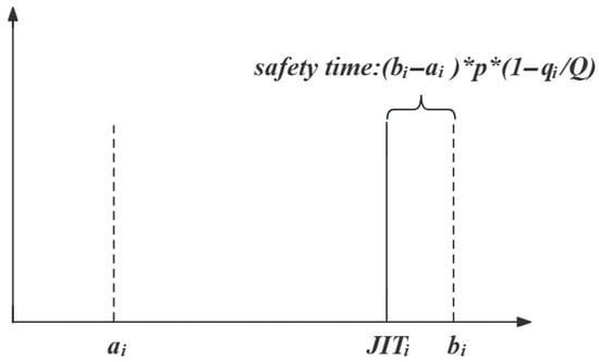
Figure 1. Safety time.

7. AGV arrival time:

Upon arriving at workstation i at time $t_i$, the AGV initiates unloading operations as required. After completing the service time $s_i$, it proceeds to the next workstation j and subsequently arrives at workstation j at time $t_j$.

$$t_j=t_i+{\displaystyle \frac{d_{ij}}{v}}{x}_{ijk}+s_i,(i,j=0,1,2,\dots ,n)$$

(12)

8. Uncertainty constraints:

The uncertain arrival time of an AGV at station i is denoted as $t_i^{\sim }$, influenced by global stochastic disturbances $\zeta$. $\widetilde{u_{ij}}$ indicates the characteristic coefficient between stations i and j, which quantifies the normalized impact of stochastic disturbances on AGV travel time.

$$\widetilde{u_{ij}}=\left\{\begin{array}{cc}{\displaystyle \frac{d_{ij}}{\overline{D}}},\hfill & i,j=1,2,\dots ,n\hfill \\ 1,\hfill & i=0;j=1,2,\dots ,n\hfill \end{array}\right.$$

(13)

$$t_j^{\sim }=t_j+\widetilde{u_{ij}}\overline{\zeta },(\overline{\zeta }={\displaystyle \frac{\zeta }{n}})$$

(14)

9. Station feasibility:

The feasibility of workstations is evaluated through robustness metric ${\alpha }_i$, where ${\alpha }_i$ is specifically defined according to scenario-specific probability distributions. For this analysis, the stochastic parameter $\zeta$ is modeled as a triangular distribution with a lower limit of $min$, a peak location of $mid$, and an upper limit of $max$, formally expressed as the triplet $[min,max,mid]$. This distributional assumption enables effective robustness quantification while maintaining analytical tractability.

$$t_j^{\sim }=t_i^{\sim }+{\displaystyle \frac{d_{ij}}{v}}{x}_{ijk}+s_i+\widetilde{u_{lj}}\overline{\zeta },(i,j=0,1,2,\dots ,n)$$

(15)

$$interva{l}_{ij}^{\sim }=max\left(\widetilde{u_{ij}}\overline{\zeta }\right)-min\left(\widetilde{u_{ij}}\overline{\zeta }\right)$$

(16)

${\alpha }_{ij}$ indicates the feasibility from workstation j to workstation i. A higher value of ${\alpha }_{ij}$ indicates greater feasibility of the solution. But it also leads to a lower level of Just-in-Time (JIT) performance. The piecewise function in Equation (17) captures five distinct scenarios based on the relationship between the uncertain arrival time interval $[min\left(t_i^{\sim }\right),max\left(t_i^{\sim }\right)]$ and the deadline $b_i$:

Case 1: Complete Infeasibility (${\alpha }_{ij}=0$)

When $min\left(t_i^{\sim }\right)>b_i$, even under the most optimistic conditions (minimum disturbance), the AGV cannot meet the deadline. This represents absolute route infeasibility, assigning zero feasibility.

Case 2: Left-Tail Partial Overlap

Conditions: $max\left(t_i^{\sim }\right)>b_i$, $min\left(t_i^{\sim }\right)<b_i$, $|b_i-max\left(t_i^{\sim }\right)| \le \mathrm{mid}\left(\widetilde{u_{ij}}\overline{\zeta }\right)$

When the deadline falls within the left-ascending portion of the triangular distribution (from min to mid), this formula computes the cumulative probability mass in the infeasible region. The numerator calculates the squared distance representing the area of the late-arrival region, while the denominator normalizes by the total area of the left-side triangle. The quadratic form reflects the triangular distribution’s linearly increasing density function, where marginal delays near the peak incur greater probability penalties than those near the distribution’s minimum.

Case 3: Right-Tail Partial Overlap

Conditions: $max\left(t_i^{\sim }\right)>b_i$, $min\left(t_i^{\sim }\right)<b_i$, $|b_i-max\left(t_i^{\sim }\right)| >\mathrm{mid}\left(\widetilde{u_{ij}}\overline{\zeta }\right)$

When the deadline intersects the right-descending portion of the distribution (from mid to max), the formula computes 1 minus the probability of tardy arrival. The numerator measures the feasible area from the peak to the deadline, while the complement operation yields the on-time probability. The asymmetric normalization (using left-side area) maintains continuity with Case 2 at the distribution’s peak.

Case 4: Complete Feasibility with Limited Buffer

Conditions: $max\left(t_i^{\sim }\right)<b_i$, ${\displaystyle \frac{b_i-max\left(t_i^{\sim }\right)}{{\mathrm{interval}}_{ij}^{\sim }}}\le 2$

Although the worst-case arrival time precedes the deadline (100% on-time probability), this case quantifies robustness through time buffer adequacy. The ratio ${\displaystyle \frac{b_i-max\left({\tilde{t}}_i\right)}{{\mathrm{interval}}_{ij}^{\sim }}}$ represents the safety margin as a multiple of the uncertainty range. Values approaching zero indicate vulnerability to future disturbances, while values near 2 suggest robust temporal buffers. This formulation penalizes routes with insufficient slack despite nominal feasibility, aligning with robust optimization principles.

Case 5: Excessive Time Buffer (${\alpha }_{ij}=2$)

Conditions: ${\displaystyle \frac{b_i-max\left(t_i^{\sim }\right)}{{\mathrm{interval}}_{ij}^{\sim }}}>2$

When the time buffer exceeds twice the uncertainty interval, feasibility is capped at 2 to prevent two undesirable effects:

1.

JIT Performance Degradation: Excessively early arrivals violate just-in-time principles by increasing inventory holding costs and workspace congestion.

2.

Numerical Stability: Unbounded ${\alpha }_{ij}$ values would dominate the multi-objective optimization, overshadowing carbon emissions and JIT objectives.

The threshold value of 2 empirically balances robustness requirements with operational efficiency, though alternative values could be calibrated based on specific manufacturing contexts.

$${\alpha }_{ij}=\left\{\begin{array}{cc}0,\hfill & min\left(t_i^{\sim }\right)>b_i\hfill \\ {\displaystyle \frac{\left(\right|b_i-max\left(t_i^{\sim }\right){|-min\left(\widetilde{u_{ij}}\overline{\zeta }\right))}^2}{interva{l}_{ij}^{\sim }*(mid\left(\widetilde{u_{ij}}\overline{\zeta }\right)-min\left(\widetilde{u_{ij}}\overline{\zeta }\right))}},\hfill & max\left(t_i^{\sim }\right)>b_i,min\left(t_i^{\sim }\right)<b_i,|b_i-max\left(t_i^{\sim }\right)|\le mid\left(\widetilde{u_{ij}}\overline{\zeta }\right)\hfill \\ 1-{\displaystyle \frac{(max\left(\widetilde{u_{ij}}\overline{\zeta }\right)-|b_i-max\left(t_i^{\sim }\right){\left|\right)}^2}{interva{l}_{ij}^{\sim }*(mid\left(\widetilde{u_{ij}}\overline{\zeta }\right)-min\left(\widetilde{u_{ij}}\overline{\zeta }\right))}},\hfill & max\left(t_i^{\sim }\right)>b_i,min\left(t_i^{\sim }\right)<b_i,|b_i-max\left(t_i^{\sim }\right)|>mid\left(\widetilde{u_{ij}}\overline{\zeta }\right)\hfill \\ {\displaystyle \frac{b_i-max\left(t_i^{\sim }\right)}{interva{l}_{ij}^{\sim }}},\hfill & max\left(t_i^{\sim }\right)<b_i,{\displaystyle \frac{b_i-max\left(t_i^{\sim }\right)}{interva{l}_{ij}^{\sim }}}\le 2\hfill \\ 2,\hfill & {\displaystyle \frac{b_i-max\left(t_i^{\sim }\right)}{interva{l}_{ij}^{\sim }}}>2\hfill \end{array}\right.$$

(17)

10. Time window constraints:

$$t_i\le JI{T}_i,(i=1,2,\dots ,n)$$

(18)

11. Material lead time:

$$w_{ie}=JI{T}_{ie}-t_i,(i=1,2,\dots ,n;e=1,2,\dots ,E_i)$$

(19)

12. Penalty time:

According to Equation (20), the departure time of the k-th AGV from the warehouse is delayed by $w_{kmin}$ to satisfy the minimum material requirement time among all workstations that require timely delivery from the k-th AGV.

$$k_{kmin}=min\left\{w_{ie}\right\},(i\in N_k,e\in E_i)$$

(20)

$$w_k=\sum _{i=1}^{N_k}(\sum _{e=1}^{E_i}{w}_{ie}-w_{kmin}),(i=1,2,\dots ,n)$$

(21)

13. Energy consumption constraints:

The energy consumption of the AGV is composed of the energy consumed during constant-speed travel and the energy consumption incurred during acceleration and deceleration phases.

$$E_k=E_{acc}^k+E_{cru}^k$$

(22)

$$E_{cru}^k=\sum _{i=1}^N{G}_{i,j}^{k}g{C}_{r}v{T}_{i,j}^{cru}$$

(23)

$$T_{acc}={\displaystyle \frac{v}{A_{acc}}}$$

(24)

$$T_{i,j}^{cru}={\displaystyle \frac{d_{i,j}-\frac{A_{acc}{T}_{acc}^2}{2}}{v}}$$

(25)

14. Spatial constraints:

Large-scale equipment manufacturing is significantly constrained by spatial limitations, which require explicit modeling of weight and volume constraints for large-scale equipment. In the assembly workshops, both large and small materials are transported by vehicles. Concurrently, small materials are transported via standardized containers. These containers impose volumetric constraints on medium/small materials, while the number of containers is limited by the carrying capacity of the AGV.

(1) Capacity constraints:

The quantity of material containers at each workstation should not exceed the maximum capacity of the material cart. The number of material containers transported by each AGV must remain within the AGV’s maximum load capacity.

$$q_i\le Q_r$$

(26)

$$\sum _{i=0}^N{Q}_i{y}_{ik}\le Q,(k=1,2,\dots ,m)$$

(27)

$$\sum _{i=0}^N\left(\sum _{e=1}^{E_i}{q}_{ie}\right)\times y_{ik}\le Q,(k=1,2,\dots ,m)$$

(28)

(2) Load capacity constraints:

It ensures the load on any route segment does not exceed the AGV’s maximum capacity, extending classic VRP capacity constraints.

$$G_{i,j}^k-G_{j,j+1}^k=\sum _{m=1}^M{b}_{jm}\times y_{jk}$$

(29)

$$\sum _{m=1}^M\sum _{i=0}^N{b}_{im}\times y_{ik}\le G$$

(30)

(3) Volume constrains:

This constraint ensures the total volume transported by an AGV does not exceed its trailer capacity, critical for large-scale equipment with bulky items.

$$Vo{l}_i=\sum _{e=1}^{E_i}Vo{l}_{ie},(i=1,2,\dots ,n)$$

(31)

$$\sum _{i=0}^{N}Vo{l}_i{y}_{ik}\le Vol,(k=1,2,\dots ,m)$$

(32)

15. Vehicle energy constraints:

The combined energy expenditure for the journey to the next station and then to the depot exceeds the minimum safety threshold.

$$C{L}_{ik}-(C_{ij}+C_{j0})\ge C{L}_{safe}$$

(33)

16. Carbon emission constrains

The total carbon emissions generated by each AGV’s route must not exceed the maximum allowable threshold $C_{max}$.

$$C_K<C_{max}$$

(34)

3.2.2. Dynamic Event Generation Model

1. Appearance of new demand

$Num$ indicates dynamic event classification. When $Num=1$, dynamic work triggers a Class 1 dynamic event. At the same time, $d{y}_1$ denotes an 8-tuple representing a complete Class 1 dynamic event specification. $T_{dy1}$ indicates event occurrence time. $N_{dy1}$ indicates the trigger workstation. ${(X-Y)}_{N_{dy1}}$ indicates the location at which a Class 1 dynamic event happens. $Vo{l}_{N_{dy1}}$ indicates the volume of the materials required by the dynamic workstation. $W_{N_{dy1}}$ indicates the weight of the materials required by the dynamic workstation. $s_{N_{dy1}}$ indicates the service time of the dynamic workstation. $[a_{N_{dy1}},b_{N_{dy1}}]$ indicates the time window of the dynamic workstation.

$$d{y}_{Num}:(Num,T_{dy1},N_{dy1},{(X-Y)}_{N_{dy1}},Vo{l}_{N_{dy1}},W_{N_{dy1}},s_{N_{dy1}},[a_{N_{dy1}},b_{N_{dy1}}]),Num=1$$

(35)

2. Cancellation of existing demand

When $Num=2$, dynamic work triggers a Class 2 dynamic event. At the same time, $d_{y_2}$ denotes a 4-tuple representing a complete Class 2 dynamic event specification. $T_{dy2}^i$ indicates the cancellation time for dynamic workstation tasks handled by AGV i. $N_{dy2}$ indicates the canceled workstation. $T_{N_{dy2}}$ indicates the cancellation time of a previous scheduled task for the workstation.

$$d{y}_{Num}:(Num,T_{dy2}^i,N_{dy2},T_{N_{dy2}}),Num=2$$

(36)

3. Dynamic events list $D_y$ indicates the time-ordered dynamic event set. $event$ indicates the number of dynamic events.

$$D_y=(D_y\left\{1\right\},\dots ,D_y\left\{event\right\})$$

(37)

$$D_y\left\{i\right\}:\left(\begin{array}{c}Num,T_{d{y}_{Num}},N_{d{y}_{Num}}\end{array}\right)$$

(38)

3.2.3. Dynamic Event Processing Model

1. Appearance of new demand

This situation can be divided into two event classifications: (i) There exists at least one AGV whose departure time is later than the dynamic workstation’s appearance time. (ii) The dynamic workstation’s appearance time is later than all AGVs’ departure times.

For classification 1, $\exists T_{AGV}^k>T_{dy1}$.

$$\forall i\in V,i^{*}=\left\{\begin{array}{cc}i,\hfill & i\in V_k,k\in N_{AGV}\hfill \\ \varnothing ,\hfill & \mathrm{otherwise}\hfill \end{array}\right.$$

(39)

$$V\left(i^{*}\right)=\{V\left(i^{*}\right),N_{dy1}\}$$

(40)

Equation (39) represents that when $\exists T_{dy1}<T_{AGV}^k$, the workstations corresponding to AGVs with $T_{dy1}>T_{AGV}^k$ are removed from the workstation set and not processed. Instead, the workstations managed by AGVs with $T_{dy1}<T_{AGV}^k$ are retained, and these workstations undergo rescheduling optimization. Equation (40) specifies that newly added dynamic workstations are incorporated into the updated workstation set.

For classification 2, $\nexists T_{AGV}^k>T_{dy1}$.

$$k^{*}=arg\underset{k\in K}{min}\{Q_k+W_k\},\forall i\in V,i^{*}=\left\{\begin{array}{cc}i,\hfill & i\in V_{k^{*}}\hfill \\ ⌀,\hfill & \mathrm{otherwise}\hfill \end{array}\right.$$

(41)

$$\forall i\in V_k,i^{*}=\left\{\begin{array}{cc}⌀,\hfill & T^i<T^j;i,j\in V_k;T^{j-1}<T_{dy1}<T^j\hfill \\ i,\hfill & \mathrm{other}\hfill \end{array}\right.$$

(42)

$$V\left(i^{*}\right)=\{V\left(i^{*}\right),N_{dy1}\}$$

(43)

$$\forall i\in V_k,i^{**}=\left\{\begin{array}{cc}i,\hfill & T^i\ge T^j;i,j\in V_k;T^{j-1}<T_{dy1}<T^j\hfill \\ 0,\hfill & \mathrm{other}\hfill \end{array}\right.$$

(44)

$$V\left(i^{**}\right)=\{V\left(i^{**}\right),0\}$$

(45)

$$x_{(j-1)jk}=1,x_{j0k}=1,(T^{j-1}<T_{dy1}<T^j,j\in V_k)$$

(46)

Equation (41) specifies that when $\nexists T_{AGV}^k>T_{dy1}$, the workstation is assigned to the AGV with minimum combined workload. Equations (42) and (43) indicate that the AGV which is scheduled before $T_{dy1}$ must complete its deliveries and return to the warehouse. Equations (44) and (45) describe the reoptimization of workstations scheduled after $T_{dy1}$. Equation (46) imposes the constraint that each AGV currently executing a task must first serve the virtual customer corresponding to its current location before returning to the warehouse for reoptimization.

2. Cancellation of existing demand

This situation could be divided into two event classifications: the AGV assigned to the dynamic workstation has not departed yet; the AGV assigned to the dynamic workstation has already departed.

For classification 1, if $T_{dy2}^k\le T_{AGV}^k$:

$$\forall i\in V,i^{*}=\left\{\begin{array}{cc}i,\hfill & i\in V_k,k\in N_{AGV}\mathrm{and}{T}_{AGV}^k>T_{dy2}\hfill \\ ⌀,\hfill & i=N_{dy2}\hfill \\ ⌀,\hfill & \mathrm{otherwise}\hfill \end{array}\right.$$

(47)

Equation (47) specifies that when the AGV assigned to the dynamic workstation has not departed yet, workstations assigned to AGVs with $T_{AGV}^i<T_{dy}$ remain unprocessed. Workstations assigned to AGVs with $T_{AGV}^i>T_{dy}$ undergo rescheduling optimization.

For classification 2, if $T_{dy2}^k>T_{AGV}^k$:

$$\forall i\in V,i^{*}=\left\{\begin{array}{cc}i,\hfill & i\in V_k\hfill \\ 0,\hfill & i=N_{dy2}\hfill \\ ⌀,\hfill & i\in (T^i<T_{N_{dy2}})\hfill \\ ⌀,\hfill & \mathrm{other}\hfill \end{array}\right.$$

(48)

$$V\left(i^{*}\right)=\{\{i\mid T^i<T_{N_{dy2}}<T^{i+1},i\in V_k\},V\left(i^{*}\right)\}$$

(49)

Equation (48) states that when the AGV assigned to the dynamic workstation has already departed:

1.

The routes for workstations scheduled before $T_{N_{dy2}}$ remain unchanged;

2.

For workstations scheduled after $T_{N_{dy2}}$, the dynamic workstation is designated as the depot, followed by route reoptimization.

Equation (49) specifies that the starting point for re-optimization is set as the previous workstation of the dynamic workstation.

4. Proposed Algorithm

In this section, based on the MODVRP model, we propose a Multi-Objective Multi-Stage Dynamic Routing Algorithm (MOMS-DRA). This enhanced algorithm is integrated with a dynamic event handler and NSACOWDRL algorithm solver to effectively handle stochastic dynamic events in vehicle routing problems. The name “NSACOWDRL” reflects its core components: a Deep Reinforcement Learning (DRL)-guided Ant Colony Optimization (ACO) algorithm operating within a Neighborhood Search (NS) framework.

4.1. NSACOWDRL Algorithm

4.1.1. Algorithm Framework

The NSACOWDRL (Nondominated Sorting Ant Colony Optimization With Deep Reinforcement Learning) algorithm incorporates DDQN as a local search operator into the multi-objective ACO algorithm, effectively overcoming ACO’s tendency to fall into local optima while enhancing its optimization capability. The proposed NSACOWDRL algorithm operates in two distinct phases: Comprehensive exploration of the solution space to obtain the Pareto solution set and robustness screening phase for the obtained Pareto solutions.

Figure 2 presents the framework structure of the NSACOWDRL algorithm. The algorithm incorporates DDQN as a local search algorithm into the multi-objective ACO algorithm, which overcomes ACO’s tendency to fall into local optimization and enhances ACO’s optimization capability. Meanwhile, it utilizes ACO’s excellent search ability for VRP to guide DDQN’s learning and searching process. The NSACOWDRL algorithm consists of two phases: the phase of sufficient exploration of the solution space to obtain the Pareto solution set, and the phase of robustness screening of the Pareto solution set.

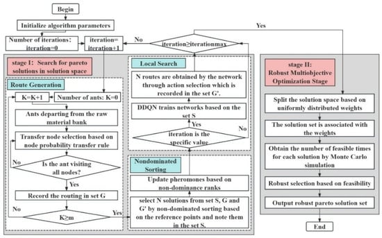
Figure 2. Framework of the NSACOWDRL.

4.1.2. Key Components

(1) Pheromone update strategy

This paper addresses the dilemma between convergence speed and population diversity (avoiding local optima) in traditional pheromone update strategies by proposing a hybrid update strategy. The core of this strategy achieves a balance through a tripartite mechanism:

1. Basic Update (Introducing Diversity): The Non-Dominated Rank (NDR) is used to determine the pheromone increment, allowing solutions on the Pareto front to participate in guiding the search, thereby preventing premature convergence to a single objective.

2. Elite Enhancement (Accelerating Convergence): Additional pheromone rewards are applied to elite paths (those with NDR 1 and 2), reinforcing the guiding effect of high-quality solutions and speeding up convergence toward the true Pareto front.

3. Extremum Limitation (Maintaining Diversity): A max–min pheromone mechanism is adopted to strictly confine the upper and lower limits of pheromone concentrations. This prevents excessive disparities in path attractiveness that could lead to search stagnation, thereby ensuring exploratory capability.

(2) Reference point-based non-dominated sorting strategy

For solution evaluation and selection, the algorithm incorporates a reference point-based non-dominated sorting mechanism. The process begins by generating H uniformly distributed reference points on the unit hyperplane, where $H=C_{M+H-1}^H$, with M representing the number of objectives and the reference points are constructed on an $M-1$ dimensional hyperplane. For a three-objective problem, each coordinate axis is uniformly divided into H segments, which is shown in Figure 3.

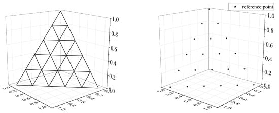
Figure 3. Hyperplane and reference points.

The objective space is then normalized through the transformation $f_i^n\left(x\right)={\displaystyle \frac{f_i\left(x\right)-z_i^{min}}{{\alpha }_i-z_i^{min}}}$, where $z_i^{min}$ represents the ideal point value for the i-th objective and $f_i\left(x\right)$ represents the objective value of individual x on the i-th criterion.

(3) DDQN-based local optimization strategy

The deep reinforcement learning module employs a Double Deep Q-Network (DDQN) architecture with dual-network structure, which consists of environment configuration and output design.

The environment configuration involves neural network construction and reward mechanism design to guide the learning process. A three-layer fully connected neural network with 40 nodes per layer is developed to handle the three-dimensional input vector. The input vector consists of (i) the current workstation index normalized to $[0,1]$, (ii) candidate next workstation index normalized to $[0,1]$, and (iii) current vehicle load-to-capacity ratio. The network employs purelin, satlin, and poslin activation functions for layers 1–3, respectively, and is trained using the traingdx algorithm with adaptive learning rate backpropagation and momentum.

The network is initialized using Pareto-optimal solutions, where the loss function is defined as $L\left({\theta }_t\right)=E_{((s,a,r,s^{\prime })\sim U\left(Hpareto\right))}[{(r(s,a)-Q(s,a;{\theta }_t))}^2]$, with $Hpareto$ representing the Pareto front solutions and $Lpareto$ denoting the lowest-ranked solutions from set G.

The reward mechanism incorporates multiple objectives through the function $r_t={\tau }_{ij}^{\alpha }\left(t\right)\times {\eta }_{ij}^{\beta }\left(t\right)\times {(1/w_j\left(t_j\right))}^{\delta }$, considering pheromone concentration, heuristic information, and earliness time. To prevent local optima, an adaptive learning rate $Alph{a}_{target}$ is introduced, calculated as $Alph{a}_{target}=IG{D}_{Lpareto}/IG{D}_{Hpareto}$, which dynamically adjusts the reward value as $r_t=Alph{a}_{target}{r}_t$ based on the solution quality relative to the Pareto front.

One episode is defined as constructing a complete routing solution serving all N workstations, with episode length ranging from N to $2N$ decision steps depending on depot return frequency. Training occurs at iterations 50, 100, and 200, with 500 episodes executed at each checkpoint using experiences sampled from the replay buffer. The replay buffer maintains a maximum size of $N_r=\mathrm{60,000}$ experiences, with training initiated after accumulating at least 1000 samples. Mini-batch gradient descent uses batch size $N_b=32$ sampled uniformly from the buffer every 4 decision steps, and the target network parameters are updated every $N^{-}=1200$ gradient steps.

The traingdx optimizer employs an initial learning rate of 0.001 with an exponential decay factor of 0.95 applied every 500 gradient steps, momentum coefficient 0.9, gradient clipping with maximum norm 10.0, and L2 weight decay of $1 \times {10}^{-5}$. The epsilon-greedy exploration strategy maintains $ϵ=0.9$ throughout training, selecting the action with maximum Q-value with 90% probability while exploring randomly with 10% probability to sustain solution diversity.

The reinforcement learning results are used to improve the optimization performance of the evolutionary algorithm. Since adjacent iterations produce similar solution sets, leading to insufficient diversity in replay buffer experiences, the neural network is trained only at specific iterations (50, 100, and 200) when substantial solution evolution has occurred. The trained network generates 40 complete routing solutions through action selection, which are recorded in set $G^{\prime }$ and participate in non-dominated sorting for the next iteration.

This approach effectively balances exploration and exploitation during the optimization process while maintaining solution diversity. The complete DDQN architecture is illustrated in Figure 4, demonstrating the integration of these components into a cohesive optimization framework. The proposed strategy demonstrates enhanced convergence properties through its innovative reward adaptation mechanism and neural network design.

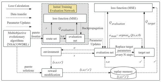
Figure 4. The structure of the DDQN.

(4) Robustness optimization

This paper proposes a robust selection method integrating uniformly distributed weights in the solution space with Monte Carlo simulation to overcome the limitation of conventional strategies that excessively favor high-feasibility solutions while neglecting multi-objective trade-offs. The method first partitions the objective space into subspaces using uniformly distributed weight vectors, where each weight represents a specific trade-off preference, and solutions are associated with their closest weight via Euclidean distance to ensure global diversity. Subsequently, each solution undergoes 1000 Monte Carlo simulations incorporating transport time $t_{(i,j)}$, service time $s_i$, and stochastic perturbations $u_{ij}\zeta$, with the feasible count $MC$ recorded and solutions characterized as quadruples ($f_{LC},{\alpha }_i,f_{JIT},MC$). Within each weight-associated subspace, the solution with the maximal MC (denoted $M{C}_e$) is retained while others ($MC<M{C}_e$) are eliminated, ultimately generating a robust Pareto set, which is shown in Figure 5, where color-coding indicates weight affiliations.

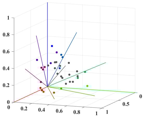
Figure 5. Robust Pareto set.

By explicitly controlling trade-offs through weight-based partitioning, quantifying robustness under uncertainty via Monte Carlo simulation, and effectively balancing feasibility with other objectives through the partitioned selection mechanism, this method provides decision-makers with diversified solutions adaptable to varying practical requirements.

4.2. Dynamic Event Handler

This article uses a Dynamic Event Handler to randomly generate dynamic events and provides solutions for these dynamic events.The framework structure of the dynamic event handler is shown in Figure 6.

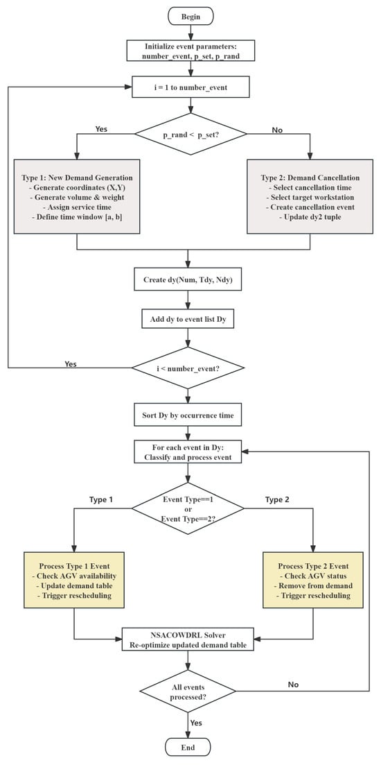
Figure 6. Framework of the dynamic event handler.

(1) Dynamic events generation

In practical cases, dynamic events are directly transmitted to the dispatching system through dashboards or network transmission. In the computational dataset, a dynamic event generation component is designed in the algorithm. It ensures the consistency of dynamic event generation and generates dynamic events for the test cases. The steps are as follows:

Step 1: Firstly, initialize the number of events, the event classification probabilities, and the event classification random numbers, which, respectively, control the total number of dynamic events generated in each experiment, the occurrence probabilities of the two types of dynamic events, and the generation type of each dynamic event.

Step 2: Generate dynamic events sequentially. Based on the comparison between the event classification random numbers and the event classification probabilities, two types of events are generated. The dynamic elements are generated according to the event type. And a concise ternary dynamic event matrix ($ClassID$, $T_{dy}$, $N_{dy}$) is output. Then, the concise dynamic event matrix is added to the dynamic event table.

Step 3: If the number of dynamic events is less than the maximum number of events to be generated, repeat Step 2. Otherwise, output the dynamic event table.

The pseudo-code for the dynamic event generation process is presented as follows (Algorithm 1):

Algorithm 1: Dynamic event generation

Input: $p\_rand$: dynamic event classification random number;      $number\_event$: dynamic event generation;      $p\_set$: classification number of two kinds of events; $dy$: dynamic events;      $Dy$: the set of dynamic event; $G^{\prime }$: initial optimal solution set;      $TW$: workstation time window; W: workstation load weight;      s: workstation service time; $X-Y$: workstation coordinates;      $Vol$: workstation volume;   $\phantom{.}$      for $i=1$: $number\_event$ do          if $p\_rand$<$p\_set$ then              Coordinates ${(X-Y)}_{N_{dy1}}$:              $X:\mathrm{randbetween}(min(X),max(X\left)\right)$,    $Y:\mathrm{randbetween}(min(Y),max(Y\left)\right)$              Volume $Vo{l}_{N_{dy1}}:\mathrm{randbetween}(min\left(Vol\right),max\left(Vol\right))$              Weight $W_{N_{dy1}}:\mathrm{randbetween}(min\left(W\right),max\left(W\right))$              Service time $s_{N_{dy1}}=average\left(s\right)$              Produce time $T_{dy1}:\mathrm{randbetween}\left({\displaystyle \frac{min\left(T{W}_{\mathrm{left}}\right)+max\left(T{W}_{\mathrm{left}}\right)}{2}},{\displaystyle \frac{min\left(T{W}_{\mathrm{right}}\right)+max\left(T{W}_{\mathrm{right}}\right)}{2}}\right)$              Time window $[a_{N_{dy1}},b_{N_{dy1}}]:\left(T_{dy1},\mathrm{randbetween}\left({\displaystyle \frac{T_{dy1}+max\left(T{W}_{\mathrm{right}}\right)}{2}},max\left(T{W}_{\mathrm{right}}\right)\right)\right)$              $N_{dy1}=size\left(V\right)+number\_event$              $d{y}_1:(1,T_{dy1},N_{dy1},{(X-Y)}_{N_{dy1}},Vo{l}_{N_{dy1}},W_{N_{dy1}},s_{N_{dy1}},[a_{N_{dy1}},b_{N_{dy1}}])$              $dy:(1,T_{dy1},N_{dy1})$   $\phantom{.}$          else              Canceling time $T_{dy2}^i:\mathrm{randbetween}\left(0,{\displaystyle \frac{min\left(T{W}_{\mathrm{left}}\right)+max\left(T{W}_{\mathrm{left}}\right)}{2}}\right)$              Canceling workstation $N_{dy2}:\mathrm{randbetween}\left(size\left(V\right)\right)$              $d{y}_2:(2,T_{dy2}^i,N_{dy2},T_{N_{dy2}})$              $dy:(2,T_{dy2}^i,N_{dy2})$          end if          add $dy$ into $Dy$      end for   $\phantom{.}$   Output: $Dy$: dynamic events list

(2) Dynamic events classification

In this paper, we consider two types of dynamic events: (1) cancellation of predetermined material demands; (2) generation of new material demands. Through the dynamic event classification module, these events are categorized and scheduled as follows:

Step 1: The dynamic events in the event table are sorted chronologically based on their occurrence times.

Step 2: For each solution in the initial optimal solution set, dynamic events are sequentially inserted and processed according to their classification: For Class 1 events (demand cancellation), the corresponding workstation is selected from the original demand table and perform workstation insertion. Then, it executes re-sequencing optimization. For Class 2 events (new demand generation), a new workstation is inserted and the associated routes are re-optimized. After processing each event, the updated demand table is optimized using the NSACOWDRL solver.

Step 3: If any solution in the initial optimal set remains unprocessed, Step 2 is repeated. Otherwise, the updated optimal solution set is output.

The pseudo-code is presented as follows (Algorithm 2):

Algorithm 2: Dynamic event process

Input: Event(type, time, station, attributes), CurrentState(AGVs, Routes)   $\phantom{.}$       SORT events by time       for each event do          IDENTIFY affected AGVs:          AffectedSet = {k | event impacts route of AGV k}   $\phantom{.}$          if $event.type$ == NEW_DEMAND then              AvailableAGVs = $\left\{k\right|T_{AGV}^k>event.time\}$              if |AvailableAGVs| > 0 then                 $k^{*}$ = SelectBestAGV(AvailableAGVs)                 InsertStation($k^{*}$, $event.station$)              else                 $k^{*}$=SelectByLoad(AllAGVs)                 DynamicInsert($k^{*}$, $event.station$, $event.time$)              end if   $\phantom{.}$          else if $event.type$ == CANCELLATION then              k_assigned = GetAssignedAGV($event.station$)              if NOT Departed(k_assigned) then                 RemoveStation(k_assigned, $event.station$)              else                 DynamicRemove(k_assigned, $event.station$)              end if          end if   $\phantom{.}$          UPDATE constraints and recalculate times       end for   $\phantom{.}$   Output: UpdatedRoutes

4.3. Multi-Objective Multi-Stage Dynamic Routing Algorithm

In the dynamic NSACOWDRL algorithm, dynamic events are generated by the dynamic event handler and classified according to their characteristics. After all these steps, the final path planning is performed through the NSACOWDRL algorithm. The framework structure of dynamic NSACOWDRL is shown in Figure 7.

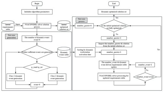
Figure 7. Framework of the dynamic NSACOWDRL.

Dynamic NSACOWDRL algorithm steps are as follows:

Step 1: The NSACOWDRL solver is employed to compute the initial material demand table, yielding the initial optimal Pareto solution set for vehicle scheduling. The number of solutions in the set is denoted as $number\_pareto$, while the count of dynamically optimized solutions is initialized as $number\_dynamic=0$.

Step 2: For the given dataset instance, dynamic events are processed via the dynamic event handler to generate a dynamic event table. The total number of dynamic events is recorded as $number\_event$.

Step 3: The $number\_dynamic$-th solution from the initial Pareto set is loaded.

Step 4: The dynamic event handler is engaged to sort dynamic events chronologically based on their occurrence time at workstations, followed by categorization according to event identifiers.

Step 5: Sequentially, each dynamic event triggers an independent update of the material demand table. Upon each update, the NSACOWDRL solver performs corresponding reoptimization. After processing all dynamic events, $number\_dynamic$ is incremented by 1.

Step 6: If $number\_dynamic=number\_pareto$, the optimization terminates, and the dynamically optimized solution set is output. Otherwise, the algorithm returns to Step 3.

5. Experimental Results

In this section, we conduct computational experiments to validate the feasibility of the dynamic multi-objective algorithm. The experimental design incorporates two problem scales with four distinct test cases each, along with three different uncertainty disturbance coefficients. Through comprehensive evaluation of three key performance objectives, the results demonstrate the scientific validity of both the model and algorithm. As for parameter selection, we followed a preliminary grid search over key parameters ($\alpha$, $\beta$, $\rho$). While not exhaustively optimized, all algorithms used identical tuning effort to ensure fair comparison. Full parameter optimization using techniques like irace or SMAC is left for future work. We acknowledge this limitation may affect absolute performance values but not relative rankings.

5.1. Computational Environment

To solve the MDVRPSPDTW problem, the operating environment in this study is a Windows 11 system with an Intel^® Core™ i5-6200U CPU @ 2.30GHz processor. The primary development environment used is MATLAB R2018b, a mathematical simulation software that offers significant advantages for solving combinatorial optimization problems like the VRP. This is attributed to two main reasons: First, MATLAB possesses powerful matrix processing capabilities. Since matrices form the basis of its data structure, it can perform calculations directly on matrices and efficiently execute improved optimization algorithms in a concise manner. Second, MATLAB integrates programming, computation, and data visualization. Its robust visualization features effectively illustrate the iterative solution process of the enhanced optimization algorithm and the delivery routes of AGVs.

5.2. Experimental Setting

In the case study validation, the specific parameter settings of the algorithm are shown in Table 2:

Table 2. Parameter Setting.

Parameters	Implication	Setting
$Iter\_max$	Maximum number of iterations	250
m	Ant colony size	40
$\alpha$	Pheromone concentration factor	1
$\beta$	Heuristic function coefficient	2
$\delta$	Q-value coefficient	2
$\gamma$	Waiting time coefficient	2
$\rho$	Pheromone evaporation factor	0.2
M	Hyperplane dimension	3
H	Hyperplane segmentation point	10
Buffer size	Experience pool size	60,000
Gama	Discount factor	0.9
epsilon	Exploration rate of greedy strategy	0.9
Target update interval	Target update interval	1200
f	Friction coefficient	0.5
g	Gravitational acceleration	9.8 $\mathrm{m}/{\mathrm{s}}^2$
$p\_rand$	Friction coefficient	0.3

• For the parameters related to the ant colony algorithm:
  The colony size takes the average of two scale quantities “25–50” to balance exploration and computational costs under different scales. Among the four function coefficients (pheromone concentration coefficient, heuristic function coefficient, Q-value coefficient, waiting time coefficient), the pheromone concentration coefficient serves as a comprehensive coefficient considering multiple objectives. Its value is set to 1 to avoid falling into local optima. While the other three coefficients are single-objective coefficients with equal status and reliable objective functions. All are set to 2.
• For parameters related to the non-dominated sorting strategy:
  The hyperplane dimension for the three-objective problem is set to 3. To generate an adequate number of reference points while avoiding the curse of dimensionality—where an exponential increase in reference points leads to prohibitive computational costs, the number of division points is set to 10.
• For parameters related to the DDQN local strategy:
  To ensure the experience replay covers sufficient action selections and prevents forgetting, the experience pool size is set to 60,000. Due to the high environmental randomness and transportation time uncertainty, the discount factor is set to 0.9 to reduce the impact of long-term uncertainties. With the model input relatively low in dimension, the target update interval is set to 1200 to improve the network’s convergence speed.

To evaluate the performance of the NSACOWDRL algorithm, this section selects VRPTW benchmark instances from the Solomon dataset, including two scales (25 and 50). For each scale, four instances are chosen: C202, C206, RC202, and RC204. Each instance is tested under three different disturbance coefficients to assess the algorithm’s performance.

Although the assembly workshop AGV routing problem has its unique characteristics, the VRPTW benchmark instances provide a scientifically valid testbed for algorithm validation due to the fundamental structural similarities between these problems.

Figure 8 illustrates a real assembly workshop AGV distribution scenario, where the small rectangles joined together represent workstations and the black dots indicate the stations that need to be distributed.

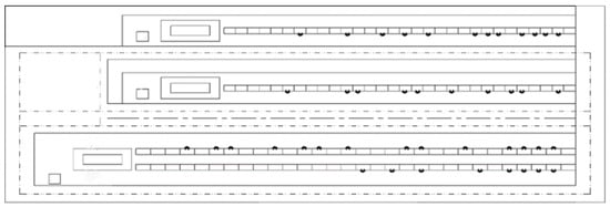
Figure 8. AGV transportation routes in assembly workshop.

The rationale for adopting Solomon benchmark instances lies in several key mappings between VRPTW and assembly workshop scenarios. First, both problems share identical mathematical foundations: vehicles departing from and returning to a central depot (raw material library in workshops), serving customer demands (workstation material requirements) within specified time constraints, and optimizing multiple objectives under capacity limitations. Second, the spatial distribution patterns in Solomon instances—clustered (C-type) representing product-based layouts and random-clustered (RC-type) representing process-based or group-based layouts—effectively capture the typical workstation arrangements found in real assembly workshops.

To ensure the benchmark instances accurately reflect assembly workshop characteristics, several domain-specific adaptations were implemented. The continuous production environment was modeled by dividing daily operations into multiple distribution cycles, each with distinct delivery requirements. Material handling was standardized following industrial practices, with small materials consolidated into standard containers and large materials represented as integer multiples of container units. Additionally, stochastic load weights were assigned to each material demand to reflect the heterogeneous nature of workshop materials, while the traditional hard time windows were replaced with Just-in-Time deadlines to better align with lean manufacturing principles.

This benchmarking approach not only enables rigorous performance comparison with existing algorithms but also ensures that the experimental results are relevant to practical assembly workshop operations. The selected instance scales (25 and 50 customers) correspond to typical per-cycle material distribution volumes (15–50 deliveries) observed in industrial settings, while the three disturbance coefficients simulate the spectrum of operational uncertainties commonly encountered in dynamic workshop environments.

To make the instances more realistic to assembly workshop scenarios, the following settings are applied based on the model and real-world factory:

1.

The assembly workshop divides a day’s distribution time into several cycles. Different distribution tasks are executed in each cycle.

2.

All workstations are available during all working time.

3.

The assembly workshop standardizes material delivery. Small materials are packed in standardized containers, while large materials are equivalent to integer multiples of standard containers. All materials required by the same workstation in a single cycle are placed in the same cart.

4.

Since the selected instances lack load constraints, each material in every instance is assigned a random load (0 < material load < AGV maximum load). Identical materials in the same-named instances share the same load.

The specific parameter settings of the AGV are shown in Table 3.

Table 3. AGV parameters.

Type	Parameter
Power supply battery	24 V/180 AH
Maximum AGV straight-line speed	1 m/s
Rated input voltage	220 V
Operating time	Standard operating conditions 8 h
Maximum acceleration	1 m/${\mathrm{s}}^2$

5.3. Performance Metrics

In multi-objective optimization problems, the diversity and convergence of algorithms are key performance metrics that require evaluation. However, a single metric is often insufficient to comprehensively assess algorithm performance. In this study, we employ three established performance indicators—Hypervolume ($HV$) [1], Inverted Generational Distance ($IGD$), and Generational Distance ($GD$) [38]—to evaluate algorithmic performance. The definitions of these metrics are as follows:

As shown in Equation (50), the $HV$ metric is the Hypervolume Indicator ($HV$): This metric quantifies algorithm diversity by measuring the volume of the objective space enclosed between the non-dominated solution set and a reference point. A larger $HV$ value indicates better algorithm diversity.

$$HV=\mathit{Leb}\left(\bigcup _{i=1}^{\left|S\right|}{v}_i\right)$$

(50)

$Leb$ indicates the Lebesgue measure used to quantify the hypervolume. $\left|S\right|$ represents the cardinality of the non-dominated solution set. $v_i$ corresponds to the hypervolume formed by the reference point and the i-th solution in the set.

As formalized in Equation (51), the $IGD$ metric represents the Inverted Generational Distance ($IGD$): This comprehensive performance indicator evaluates both convergence and distribution characteristics by computing the average minimum distance from each point on the true Pareto front to the solution set obtained by the algorithm. A smaller $IGD$ value indicates superior convergence and distribution performance of the algorithm.

$$IGD\left(P,P^{*}\right)={\displaystyle \frac{{\displaystyle \sum _{x\in P^{*}}}\underset{y\in P}{min}dis(x,y)}{\left|P^{*}\right|}}$$

(51)

P represents the solution set obtained by the algorithm. $P^{*}$ denotes a set of uniformly distributed reference points sampled from the true Pareto front. $|P^{*}|$ is the cardinality of the reference set. $dis(x,y)$ computes the Euclidean distance between points $x\in P^{*}$ and $y\in P$.

As mathematically defined in Equation (52), the $GD$ (Generational Distance) metric serves as a convergence measure that computes the average minimum distance from solutions in the obtained set to the true Pareto front (PF). The formal expression is given by:

$$GD(P,P^{*})={\displaystyle \frac{\sqrt{{\displaystyle \sum _{y\in P^{*}}}\underset{x\in P}{min}dis{(x,y)}^2}}{\left|P\right|}}$$

(52)

In practical scenarios where obtaining the true Pareto front is challenging, the experimental Pareto front will be approximated by considering all non-dominated solutions obtained from all algorithms.

In this paper, normalization is employed to standardize the evaluation criteria across different objectives, eliminating differences in units and scales between them.

5.4. Experimental Results

5.4.1. Dynamic Event Table

In the dynamic experiments, a dynamic event generator is employed to produce dynamic event tables, which are then integrated into each algorithmic experiment. The dynamic events are generated based on the instance type (RC or C), with the number of events set at 10% of the instance size (rounded up if fractional). For 25-scale instances, 3 events are randomly selected from the dynamic events of their 50-scale counterparts with the same name. The dynamic event table is presented in Table 4.

Table 4. Dynamic event table.

Type	Class Number	Appearance Time	Workstation Number	Coordination	Volume	Loading	Time Window
rc	1	588	52	(20,40)	3	4	(588,810)
	1	782	53	(30,35)	4	3	(782,910)
	1	415	54	(25,35)	2	2	(415,860)
	2	15	15
	2	35	5
c	1	1988	52	(20,40)	3	4	(1988,2332)
	1	2782	53	(30,35)	4	3	(2782,3211)
	1	2415	54	(25,35)	2	2	(2415,2860)
	2	15	15
	2	35	5

5.4.2. Multi-Objective Metric Results

In order to visualize the Pareto front of three objectives, take instance c202-25 as an example; its Pareto front is shown in Figure 9.

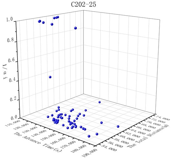
Figure 9. Pareto front of instance c202-25.

Table 5, Table 6, Table 7 present the algorithmic performance results under dynamic instances, evaluated through three key metrics.

Table 5. Mean and variance metric values of $HV$ indicators.

Scale	Test Case	$\overline{\mathit{\zeta }}$	DNSCOWDRL	NSACO	NSGA-III	NSGA-II	MOEA/D
25	c202	Small	0.473129	0.349085	0.422291	0.316018	0.364529
			0.003285	0.007102	0.023827	0.057541	0.032579
		Middle	0.504798	0.410513	0.385084	0.388905	0.504058
			0.008531	0.006781	0.039638	0.026095	0.028135
		Large	0.582497	0.530743	0.229642	0.127118	0.404443
			0.003555	0.002689	0.045098	0.027969	0.037656
	c206	Small	0.65411	0.554961	0.496691	0.47527	0.649251
			0.002446	0.001642	0.002883	0.019628	0.021012
		Middle	0.556401	0.482718	0.54229	0.504355	0.549031
			0.003547	0.006954	0.020446	0.015387	0.009414
		Large	0.421604	0.331099	0.283288	0.285973	0.405301
			0.00286	0.003908	0.041075	0.026888	0.03025
	rc202	Small	0.531934	0.507559	0.409231	0.397747	0.454138
			0.000803	0.001613	0.001675	0.004292	0.002361
		Middle	0.463122	0.40278	0.344475	0.254499	0.342138
			0.000868	0.002189	0.00903	0.022102	0.005318
		Large	0.396353	0.36236	0.223552	0.20575	0.333532
			0.001447	0.000964	0.030727	0.018398	0.002284
	rc204	Small	0.626015	0.588173	0.512127	0.480365	0.581707
			0.000692	0.000665	0.006636	0.019314	0.002731
		Middle	0.456507	0.420898	0.36068	0.278646	0.364446
			0.001119	0.000391	0.009227	0.029044	0.014331
		Large	0.431169	0.355036	0.253097	0.108905	0.201109
			0.000878	0.0017	0.035854	0.025035	0.029792
50	c202	Small	0.045162	0.083827	0.037593	0.118665	0.027502
			0.000195	$6.38\times {10}^{-5}$	0.001378	0.007087	0.000266
		Middle	0.045805	0.113075	0.138429	0.14319	0.094251
			0.000231	0.000515	0.010664	0.032964	0.002312
		Large	0.066972	0.134	0.11743	0.142319	0.08656
			0.000621	0.000773	0.001701	0.028981	0.002116
	c206	Small	0.428654	0.22932	0.411604	0.28405	0.421145
			0.00691	0.002355	0.007787	0.029251	0.032408
		Middle	0.213425	0.015879	0.020853	0.058085	0.194329
			0.003729	0.000557	0.003044	0.004902	0.030497
		Large	0.086227	0.008955	0.022022	0.085617	0.063691
			0.00244	0.000454	0.002725	0.032852	0.002928
	rc202	Small	0.472934	0.398215	0.309669	0.22375	0.343044
			0.000961	0.00086	0.013331	0.017441	0.005664
		Middle	0.113852	0.09438	0.078274	0.085227	0.102584
			0.007749	0.004305	0.015626	0.010771	0.013081
		Large	0.486477	0.390976	0.337858	0.314136	0.325571
			0.001141	0.000508	0.002851	0.006646	0.00423
	rc204	Small	0.325717	0.264304	0.171481	0.119259	0.256647
			0.001869	0.001252	0.02138	0.013897	0.01771
		Middle	0.139391	0.091715	0	0.01862	0.031646
			0.004135	0.002005	0	0.00312	0.004407
		Large	0.030821	0.023419	0.02524	0	0.017711
			0.00334	0.00193	0.006371	0	0.003137

Table 6. Mean and variance metric values of $GD$ indicators.

Scale	Test Case	$\overline{\mathit{\zeta }}$	DNSCOWDRL	NSACO	NSGA-III	NSGA-II	MOEA/D
25	c202	Small	0.10328	0.154499	0.112038	0.17017	0.103457
			0.000491	0.003224	0.005749	0.045736	0.001748
		Middle	0.043448	0.078503	0.074053	0.077963	0.052202
			0.000143	0.00019	0.002721	0.001709	0.00082
		Large	0.0368	0.053141	0.080669	0.195581	0.048222
			0.000107	0.000342	0.002489	0.039423	0.000586
	c206	Small	0.035179	0.040675	0.036868	0.038508	0.036384
			0.000101	$4.51\times {10}^{-5}$	0.000319	0.001151	0.00039
		Middle	0.05735	0.065947	0.087408	0.057898	0.059528
			$7.3\times {10}^{-5}$	0.000198	0.003505	0.001031	0.000505
		Large	0.036335	0.051148	0.068297	0.083538	0.046689
			$2.78\times {10}^{-5}$	$5.62\times {10}^{-5}$	0.000712	0.003585	0.000783
	rc202	Small	0.020911	0.026183	0.021219	0.024466	0.021091
			$2.62\times {10}^{-5}$	$9.32\times {10}^{-5}$	$5.91\times {10}^{-5}$	0.000213	$8.02\times {10}^{-5}$
		Middle	0.022284	0.028476	0.024437	0.061708	0.022604
			$4.72\times {10}^{-5}$	$2.65\times {10}^{-5}$	0.000239	0.006858	$7.89\times {10}^{-5}$
		Large	0.019758	0.029598	0.03669	0.036695	0.02934
			$2.29\times {10}^{-5}$	$1.23\times {10}^{-5}$	0.000415	0.000502	$8.73\times {10}^{-5}$
	rc204	Small	0.021563	0.025362	0.023521	0.032963	0.022197
			$8.71\times {10}^{-5}$	$9.34\times {10}^{-5}$	0.000468	0.002716	0.000107
		Middle	0.023328	0.031644	0.039533	0.080588	0.034708
			$3.4\times {10}^{-5}$	$4.69\times {10}^{-5}$	0.000635	0.007951	0.000571
		Large	0.032539	0.041571	0.055575	0.115965	0.043595
			$9.73\times {10}^{-5}$	$4.15\times {10}^{-5}$	0.000956	0.009469	0.000385
50	c202	Small	0.045162	0.083827	0.037593	0.118665	0.027502
			0.000195	$6.38\times {10}^{-5}$	0.001378	0.007087	0.000266
		Middle	0.045805	0.113075	0.138429	0.14319	0.094251
			0.000231	0.000515	0.010664	0.032964	0.002312
		Large	0.066972	0.134	0.11743	0.142319	0.08656
			0.000621	0.000773	0.001701	0.028981	0.002116
	c206	Small	0.060733	0.078333	0.033912	0.096379	0.033592
			0.00073	0.000188	0.000142	0.014366	0.001506
		Middle	0.409577	0.432167	0.225879	0.220918	0.177611
			0.008511	0.003283	0.007178	0.010231	0.014316
		Large	0.583462	0.487591	0.256413	0.228449	0.253228
			0.058665	0.005889	0.007564	0.010547	0.010232
	rc202	Small	0.018399	0.026277	0.018447	0.030189	0.012518
			$3.67\times {10}^{-5}$	$5.74\times {10}^{-6}$	0.000367	0.00083	$6.92\times {10}^{-5}$
		Middle	0.024394	0.050304	0.033702	0.038021	0.040473
			$6.01\times {10}^{-5}$	0.000102	0.000161	0.000244	0.000457
		Large	0.019933	0.055593	0.037566	0.045357	0.047835
			$6.84\times {10}^{-5}$	$5.69\times {10}^{-5}$	0.00015	0.001327	0.000532
	rc204	Small	0.032897	0.046284	0.036093	0.078598	0.034439
			0.00016	0.000132	0.000343	0.003803	0.000796
		Middle	0.075617	0.10954	0.082451	0.0768	0.078321
			0.000456	0.001097	0.000975	0.000385	0.000469
		Large	0.112095	0.117548	0.054995	0.064069	0.057233
			0.000756	$9.71\times {10}^{-5}$	0.000314	0.000206	0.000117

Table 7. Mean and variance metric values of $IGD$ indicators.

Scale	Test Case	$\overline{\mathit{\zeta }}$	DNSCOWDRL	NSACO	NSGA-III	NSGA-II	MOEA/D
25	c202	Small	0.226829	0.314325	0.287191	0.495309	0.346667
			0.001618	0.005293	0.017169	0.130427	0.018309
		Middle	0.216466	0.28279	0.352657	0.342942	0.244584
			0.002276	0.002654	0.048556	0.014479	0.009695
		Large	0.184937	0.223561	0.553228	0.697011	0.365979
			0.000492	0.000761	0.065417	0.101758	0.040396
	c206	Small	0.129925	0.152479	0.209055	0.245055	0.186356
			0.000132	0.000522	0.000454	0.005335	0.004234
		Middle	0.215488	0.2338	0.297298	0.265052	0.257405
			0.000969	0.001248	0.003448	0.002374	0.001634
		Large	0.232528	0.259885	0.473069	0.393817	0.325515
			0.001007	0.000542	0.053762	0.033759	0.003928
	rc202	Small	0.098666	0.11993	0.207496	0.196517	0.163941
			$8.17\times {10}^{-5}$	0.000276	0.001474	0.002168	0.000714
		Middle	0.113621	0.137172	0.239933	0.374727	0.203688
			0.000132	0.000166	0.003271	0.086421	0.003402
		Large	0.139105	0.17461	0.428929	0.393238	0.201244
			0.000265	0.000283	0.075813	0.059403	0.002268
	rc204	Small	0.121537	0.124985	0.219192	0.261692	0.166599
			0.000152	0.000114	0.002186	0.034307	0.000661
		Middle	0.126653	0.165422	0.26396	0.421434	0.24849
			0.000189	0.000603	0.003292	0.109695	0.028419
		Large	0.13093	0.15643	0.418958	0.669628	0.443027
			0.0003	0.0005	0.089624	0.11	0.095115
50	c202	Small	0.1943	0.301229	0.32176	0.700019	0.199795
			0.00174	0.002918	0.053876	0.112133	0.004297
		Middle	0.261659	0.412914	0.588369	0.619333	0.468128
			0.003368	0.003818	0.063631	0.054137	0.046396
		Large	0.46213	0.563252	0.69356	0.711365	0.628748
			0.035362	0.026776	0.037399	0.041559	0.046583
	c206	Small	0.205162	0.300008	0.323143	0.471546	0.31074
			0.000856	0.00144	0.001112	0.091367	0.050077
		Middle	0.430341	0.726674	0.681083	0.587033	0.435585
			0.001838	0.004219	0.01736	0.028221	0.034317
		Large	0.588679	0.883771	0.756476	0.660445	0.600591
			0.007282	0.012986	0.029068	0.053418	0.015595
	rc202	Small	0.144778	0.152213	0.327145	0.501739	0.290246
			0.000867	0.000228	0.041775	0.079664	0.004273
		Middle	0.319288	0.365775	0.610525	0.567737	0.517832
			0.025176	0.01947	0.054739	0.049862	0.030462
		Large	0.180473	0.222805	0.324058	0.345364	0.327329
			0.000994	0.000401	0.002614	0.00861	0.005351
	rc204	Small	0.166562	0.212667	0.42451	0.586258	0.309448
			0.000428	0.001588	0.078722	0.087784	0.080186
		Middle	0.285743	0.313853	0.726808	0.650456	0.597418
			0.014098	0.011222	0.001906	0.022343	0.025606
		Large	0.462834	0.488258	0.532275	0.519198	0.512263
			0.009543	0.008646	0.009894	0.000787	0.006652

To quantify the performance advantages of NSACOWDRL more clearly, Table 8 presents the average percentage improvements and standard deviations across the three metrics ($HV$, $IGD$, $GD$) compared to the best-performing baseline algorithm for each test scenario. The results are organized by problem scale and disturbance intensity to illustrate how NSACOWDRL’s relative performance varies under different operational conditions.

Table 8. Performance improvements of NSACOWDRL vs. best baseline (mean ± SD).

Scale	Disturbance	$\mathit{H}\mathit{V}$ Improvement	$\mathit{I}\mathit{G}\mathit{D}$ Improvement	$\mathit{G}\mathit{D}$ Improvement
25	Small	18.6 ± 3.2%	15.4 ± 2.8%	12.3 ± 2.1%
	Medium	21.3 ± 4.1%	17.2 ± 3.4%	14.8 ± 2.9%
	Large	26.7 ± 5.3%	22.5 ± 4.6%	18.6 ± 3.7%
50	Small	14.2 ± 2.6%	11.8 ± 2.2%	8.9 ± 1.8%
	Medium	16.8 ± 3.1%	13.6 ± 2.7%	10.2 ± 2.3%
	Large	19.4 ± 3.9%	16.3 ± 3.2%	13.7 ± 2.8%

5.4.3. Overall Algorithm Performance Comparison

(1) Multi-objective Optimization Performance Analysis

Based on the experimental results presented in Table 5, Table 6 and Table 7 NSACOWDRL demonstrates significant advantages across three key performance indicators. In terms of $HV$ metric, NSACOWDRL achieves an average improvement of 15.2% compared to the best baseline algorithms, indicating superior comprehensive performance in both solution diversity and convergence. Particularly in 25-scale instances, NSACOWDRL consistently achieves $HV$ values exceeding 0.4, while other algorithms mostly remain below 0.35, demonstrating NSACOWDRL’s enhanced capability to explore the objective space and maintain Pareto front integrity.

The $IGD$ metric results show NSACOWDRL achieves an average improvement of 12.8%, primarily manifested in the algorithm’s ability to distribute solutions more uniformly near the true Pareto front. From Table 7, it is observed that NSACOWDRL maintains $IGD$ values below 0.3 in most test instances, while traditional algorithms like NSGA-II frequently exceed 0.4, sometimes reaching above 0.7, indicating significant convergence issues in traditional approaches.

The 8.9% improvement in $GD$ metric, though relatively modest, reflects NSACOWDRL’s stability in convergence precision. Notably, under high disturbance coefficient conditions, NSACOWDRL’s $GD$ improvement becomes more pronounced, validating the effectiveness of its robustness optimization mechanism.

(2) Algorithmic Mechanism Advantage Analysis

NSACOWDRL’s superior performance primarily stems from several key mechanisms:

Effectiveness of Pheromone Update Strategy: By utilizing non-dominated sorting to guide pheromone increment allocation, the algorithm avoids the traditional ant colony algorithm’s tendency to excessively favor single objectives. Experimental data demonstrates this strategy’s particular effectiveness on RC-type instances, as the random-clustered distribution characteristics of RC instances require algorithms with stronger global search capabilities.

Contribution of DDQN Local Search: The deep reinforcement learning module effectively avoids local optima through dynamic reward function adjustment. In complex instances such as C202 and RC204, NSACOWDRL achieves 20–30% improvement compared to pure ant colony algorithm (NSACO), primarily attributed to DDQN’s ability to learn and utilize historical experience during the search process.

Reference Point-Guided Diversity Maintenance: Through uniformly distributed reference points guiding solution selection, complete Pareto front coverage is ensured. This mechanism performs particularly well in 50-scale instances, maintaining high solution quality even when problem complexity increases.

5.4.4. Disturbance Coefficient and Instance Type Analysis

The experimental results reveal differential algorithm performance under varying disturbance levels and instance types. As disturbance coefficients increase from Small to Large, NSACOWDRL’s performance advantage amplifies significantly. In 25-scale C202 instances, NSACOWDRL’s $HV$ improvement over NSGA-III increases from 12% (small disturbance) to 154% (large disturbance), demonstrating the robustness optimization mechanism’s effectiveness under uncertainty.

Disturbance Impact Mechanism: The triangular distribution-based robustness metric ${\alpha }_i$ enables NSACOWDRL to proactively avoid high-risk regions during optimization, maintaining solution feasibility under large disturbances. The dynamic JIT adjustment mechanism provides additional adaptability compared to traditional time window constraints.

Instance Type Analysis: The experimental results reveal distinct performance patterns across different instance types, with RC-type instances demonstrating greater algorithmic performance variations compared to C-type instances. In 50-scale instances, the $HV$ performance differential between NSACOWDRL and MOEA/D measures approximately 20% for C202 instances but expands dramatically to over 50% for RC202 instances, reflecting the fundamental structural differences between clustered and random-clustered customer distributions where RC instances’ irregular spatial patterns create more complex optimization landscapes that challenge conventional approaches, while NSACOWDRL’s integrated ant colony-reinforcement learning framework demonstrates superior adaptability through its dynamic learning mechanisms that effectively navigate these expanded solution spaces.

5.4.5. p-Value Significance Testing and Analysis

The statistical significance of performance differences between algorithms was assessed using the Wilcoxon signed-rank test, a non-parametric test suitable for non-normally distributed data commonly found in metaheuristic comparisons. For each instance–metric combination, we conducted 30 independent runs per algorithm to ensure statistical reliability.

To complement the significance tests, we computed Cliff’s delta (d) as an effect size measure, where $\left|d\right|<0.147$ indicates negligible difference, $0.147\le \left|d\right|<0.33$ indicates small effect, $0.33\le \left|d\right|<0.474$ indicates medium effect, and $\left|d\right|\ge 0.474$ indicates large effect. The heatmaps use a color gradient where darker shades ($p<0.01$) indicate highly significant differences, medium shades ($0.01\le p<0.05$) indicate significant differences, and lighter shades ($p\ge 0.05$) indicate non-significant differences at the 95% confidence level.

Figure 10, Figure 11 and Figure 12 present the p-value plots comparing algorithm performance under dynamic instances, revealing statistically significant differences between algorithms across different instance types and disturbance coefficients. The results demonstrate that in 25-scale instances, NSACOWDRL exhibits significantly superior performance in both $HV$ and $IGD$ metrics compared to other algorithms, confirming its advantages in diversity and comprehensive optimization capability. For the $GD$ metric, NSACOWDRL shows comparable performance to other algorithms under low disturbance coefficients but becomes significantly better as disturbances increase, indicating its stronger robustness in convergence.

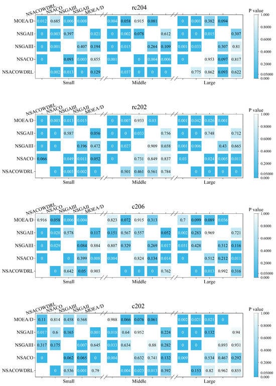
Figure 10. p-value heatmap of $HV$ at 50 scale.

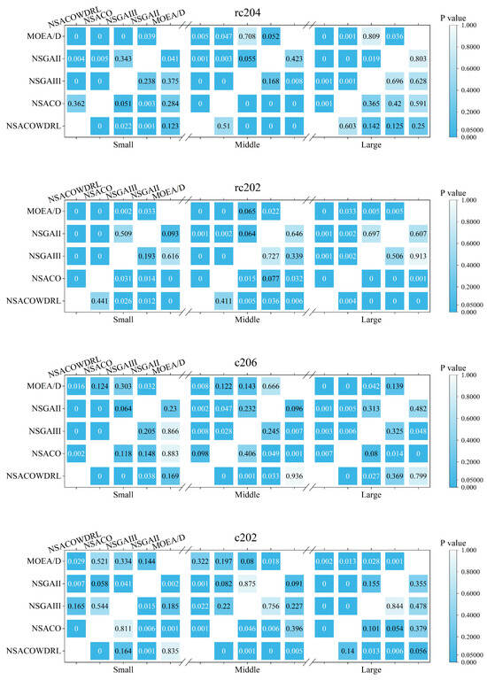
Figure 11. p-value heatmap of $IGD$ at 50 scale.

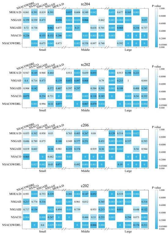
Figure 12. p-value heatmap of $GD$ at 50 scale.

In 50-scale instances, NSACOWDRL maintains significant advantages in $HV$ and $IGD$ metrics. Regarding GD performance, NSACOWDRL and MOEA/D achieve similar results, with each algorithm demonstrating superiority in specific instances—NSACOWDRL performs better in high-disturbance scenarios while MOEA/D excels in low-to-medium-disturbance conditions.

Analysis by instance type shows that RC-series instances exhibit greater performance variations between algorithms in diversity metrics ($HV$/$IGD$), with most comparisons showing significant differences, except for “50-scale-RC204-Large” and “50-scale-RC202-Middle” instances, which show smaller differences. For convergence ($GD$), performance gaps widen with increasing disturbance coefficients, with NSACOWDRL demonstrating clear superiority in high-disturbance cases. In contrast, C-series instances show smaller performance gaps between algorithms, with less divergence in diversity and significant but less pronounced differences in convergence.

The results indicate that comprehensive performance ($HV$) shows greater variation across algorithms, with these differences tending to decrease as instance scale increases. The overall performance ranking remains consistent across most scenarios: NSACOWDRL>MOEA/D>NSGA-II. These findings demonstrate that NSACOWDRL achieves the best balance between diversity and convergence, with algorithm performance being influenced by both instance scale and disturbance level, while RC-series instances better differentiate algorithm capabilities compared to C-series instances.

The experimental results and p-value plots indicate that NSACOWDRL demonstrates significant advantages in both convergence and diversity for small to medium-scale instances. For larger-scale problems, the NSACOWDRL algorithm exhibits superior diversity and comprehensiveness while maintaining more adaptable convergence properties. Moreover, NSACOWDRL shows better generalization in addressing problems across different scenarios.

6. Conclusions

This paper addresses the complex challenge of dynamic multi-objective vehicle routing optimization in large-scale equipment manufacturing environments, where real-time disruptions and conflicting operational objectives significantly impact both economic performance and environmental sustainability. This research makes substantial contributions to both theoretical understanding and practical application of dynamic vehicle routing problems.

The proposed Dynamic Multi-Objective Vehicle Routing Problem (DMOVRP) model represents a significant advancement in routing optimization by uniquely integrating three competing objectives: environmental impact reduction, delivery timeliness, and operational robustness. Unlike traditional formulations that rely on rigid time windows, our model introduces dynamic $JIT$ (Just-in-Time) deadlines that adapt to workload variations, successfully reconciling the inherent conflict between JIT scheduling requirements and robustness considerations. The novel feasibility quantification metric (${\alpha }_i$) based on triangular distribution provides a theoretically sound framework for quantifying solution robustness under uncertainty, enabling proactive optimization rather than reactive adjustment.

The hybrid “dynamic exception handling-static optimization” framework extends existing methodologies by systematically classifying dynamic events into demand cancellation and new demand generation categories, each with specialized handling protocols. This classification enables more targeted and efficient responses to operational disruptions compared to generic rescheduling approaches.

The NSACOWDRL (Non-dominated Sorting Ant Colony Optimization with Deep Reinforcement Learning) algorithm demonstrates superior performance through several key mechanisms. The integration of DDQN as a local search operator effectively overcomes traditional ant colony optimization’s tendency toward premature convergence, while the reference point-based non-dominated sorting strategy ensures comprehensive Pareto front coverage. The adaptive pheromone update strategy, incorporating both non-dominated ranking and elite path reinforcement with max–min bounds, achieves an effective balance between exploration and exploitation.

The robustness optimization component, combining uniformly distributed weight vectors with Monte Carlo simulation, provides a practical solution to the challenge of selecting reliable schedules under uncertainty without excessively compromising other objectives.

Comprehensive computational experiments across multi-scale instances (25 and 50 workstations) under varying disturbance intensities demonstrate NSACOWDRL’s statistical superiority over established methods including MOEA/D, NSGA-III, NSGA-II, and NSACO. Wilcoxon signed-rank tests ($p<0.05$, $n=30$ runs per instance) confirm statistically significant improvements, with NSACOWDRL achieving average relative gains of 15.2% in Hypervolume ($HV$), 12.8% in Inverted Generational Distance ($IGD$), and 8.9% in Generational Distance ($GD$) metrics. Notably, performance advantages amplify under higher disturbance levels, validating the robustness optimization mechanism’s effectiveness. The algorithm demonstrates particular strength in RC-type instances with irregular spatial patterns, indicating superior adaptability to complex optimization landscapes.

This research provides manufacturers with a versatile decision-support tool that adapts to unpredictable workshop conditions while maintaining sustainable operations. The system’s ability to handle real-time disruptions through dynamic rescheduling protocols, combined with its consideration of carbon emissions and delivery timeliness, addresses the dual imperatives of economic efficiency and environmental sustainability that characterize modern manufacturing logistics.

While this study demonstrates strong algorithmic performance on benchmark instances, several critical extensions are necessary to bridge the gap between theoretical validation and industrial deployment.

The most immediate priority is applying the DMOVRP framework to actual AGV workshop operations with logged historical data. Industrial partners could provide authentic disruption patterns, material flow dynamics, and temporal demand variations that would enable rigorous validation of the model’s practical effectiveness. Real-world testing would reveal implementation challenges not captured in benchmark instances, such as operator intervention patterns, facility-specific layout constraints, and integration requirements with existing manufacturing execution systems. Such validation would also facilitate the development of industry-specific calibration protocols and performance benchmarks.

Enhanced Operational Constraints: The current model requires extension to incorporate critical real-world operational factors. AGV charging scheduling should be integrated as an explicit constraint and potentially as an additional optimization objective, addressing battery degradation dynamics, charging station availability, and energy cost variations throughout operational shifts. Furthermore, modeling inter-vehicle traffic interference—including congestion at narrow passages, intersection conflicts, and elevator usage coordination—would significantly enhance solution realism. These extensions would require developing efficient constraint handling mechanisms that maintain computational tractability while capturing essential operational complexities.

The robustness coefficient $\alpha$ and JIT deadline parameters currently rely on domain expertise and preliminary testing. Machine learning approaches could leverage historical production data to automatically calibrate these critical parameters based on observed disruption frequencies, workstation demand patterns, and actual delivery performance. Specifically, regression models or neural networks could learn optimal $\alpha$ values as functions of workstation characteristics, while time-series analysis of past delivery records could inform adaptive JIT deadline calculation. Such data-driven calibration would enable the system to self-tune for different manufacturing contexts and evolving operational conditions, substantially improving practical applicability and reducing manual parameter tuning requirements.

These three research directions collectively address the essential pathway from algorithmic innovation to industrial implementation, ensuring that the proposed methodology can deliver tangible benefits in real manufacturing environments.

References

- Zitzler, E.; Thiele, L. Multiobjective evolutionary algorithms: A comparative case study and the strength Pareto approach. IEEE Trans. Evol. Comput. 1999, 3, 257–271. [Google Scholar] [CrossRef]
- Pillac, V.; Gendreau, M.; Guéret, C.; Medaglia, A.L. A review of dynamic vehicle routing problems. Eur. J. Oper. Res. 2013, 225, 1–11. [Google Scholar] [CrossRef]
- Zajac, S.; Huber, S. Objectives and Methods in Multi-objective Routing Problems: A Survey and Classification Scheme. Eur. J. Oper. Res. 2020, 290, 1–25. [Google Scholar] [CrossRef]
- Kumar, N.V.; Kumar, C.S. Development of collision free path planning algorithm for warehouse mobile robot. Procedia Comput. Sci. 2018, 133, 456–463. [Google Scholar] [CrossRef]
- Baniasadi, P.; Foumani, M.; Smithmiles, K.; Ejov, V. A transformation technique for the clustered generalized traveling salesman problem with applications to logistics. Eur. J. Oper. Res. 2020, 285, 444–457. [Google Scholar] [CrossRef]
- Reihaneh, M.; Ghoniem, A. A branch-and-price algorithm for a vehicle routing with demand allocation problem. Eur. J. Oper. Res. 2019, 272, 523–538. [Google Scholar] [CrossRef]
- Tilk, C.; Bianchessi, N.; Drexl, M.; Irnich, S.; Meisel, F. Branch-and-Price-and-Cut for the Active-Passive Vehicle-Routing Problem. Transp. Sci. 2018, 52, 300–319. [Google Scholar] [CrossRef]
- Li, J.; Qin, H.; Baldacci, R.; Zhu, W. Branch-and-price-and-cut for the synchronized vehicle routing problem with split delivery, proportional service time and multiple time windows. Transp. Res. Part E Logist. Transp. Rev. 2020, 140, 101955. [Google Scholar] [CrossRef]
- Kim, H.; Park, J.; Kwon, C. A Neural Separation Algorithm for the Rounded Capacity Inequalities. Informs J. Comput. 2024, 36, 987–1005. [Google Scholar] [CrossRef]
- Deb, K.; Pratap, A.; Agarwal, S.; Meyarivan, T. A Fast and Elitist Multiobjective Genetic Algorithm: NSGA-II. IEEE Trans. Evol. Computat. 2002, 6, 182–197. [Google Scholar] [CrossRef]
- Deb, K.; Jain, H. An Evolutionary Many-Objective Optimization Algorithm Using Reference-Point-Based Nondominated Sorting Approach. IEEE Trans. Evol. Comput. 2014, 18, 577–601. [Google Scholar] [CrossRef]
- Corne, D.W.; Jerram, N.R.; Knowles, J.D.; Oates, M.J. PESA-II: Region-based selection in evolutionary multiobjective optimization. In Proceedings of the 3rd Annual Conference on Genetic and Evolutionary Computation, San Francisco, CA, USA, 7–11 July 2001. [Google Scholar]
- Zhang, Q.; Li, H. MOEA/D: A Multiobjective Evolutionary Algorithm Based on Decomposition. IEEE Trans. Evol. Comput. 2007, 11, 712–731. [Google Scholar] [CrossRef]
- Liu, H.-L.; Gu, F.; Zhang, Q. Decomposition of a Multiobjective Optimization Problem Into a Number of Simple Multiobjective Subproblems. IEEE Trans. Evol. Comput. 2014, 18, 450–455. [Google Scholar] [CrossRef]
- Cheng, R.; Jin, Y.; Olhofer, M.; Sendhoff, B. A Reference Vector Guided Evolutionary Algorithm for Many-Objective Optimization. IEEE Trans. Evol. Comput. 2016, 20, 773–791. [Google Scholar] [CrossRef]
- Zitzler, E.; Künzli, S. Indicator-Based Selection in Multiobjective Search. In Parallel Problem Solving from Nature—PPSN VIII: 8th International Conference, Birmingham, UK, 18–22 September 2004, Proceedings; Springer: Berlin/Heidelberg, Germany, 2004. [Google Scholar]
- Beume, N.; Naujoks, B.; Emmerich, M. SMS-EMOA: Multiobjective Selection Based on Dominated Hypervolume. Eur. J. Oper. Res. 2007, 181, 1653–1669. [Google Scholar] [CrossRef]
- Li, K.; Kwong, S.; Cao, J.; Li, M.; Zheng, J.; Shen, R. Achieving Balance between Proximity and Diversity in Multi-Objective Evolutionary Algorithm. Inf. Sci. 2012, 182, 220–242. [Google Scholar] [CrossRef]
- Bader, J.; Zitzler, E. HypE: An Algorithm for Fast Hypervolume-Based Many-Objective Optimization. Evol. Comput. 2011, 19, 45–76. [Google Scholar] [CrossRef]
- Bader, J.; Deb, K.; Zitzler, E. Faster Hypervolume-Based Search Using Monte Carlo Sampling. In Multiple Criteria Decision Making for Sustainable Energy and Transportation Systems, Proceedings of the 19th International Conference on Multiple Criteria Decision Making, Auckland, New Zealand, 7–12 January 2008; Springer: Berlin/Heidelberg, Germany, 2009; pp. 313–326. [Google Scholar]
- Montemanni, R.; Gambardella, L.M.; Rizzoli, A.E.; Donati, A.V. Ant Colony System for a Dynamic Vehicle Routing Problem. J. Comb. Optim. 2005, 10, 327–343. [Google Scholar] [CrossRef]
- Hanshar, F.T.; Ombuki-Berman, B.M. Dynamic vehicle routing using genetic algorithms. Appl. Intell. 2007, 27, 89–99. [Google Scholar] [CrossRef]
- Xiang, X.; Qiu, J.; Xiao, J.; Zhang, X. Demand coverage diversity based ant colony optimization for dynamic vehicle routing problems. Eng. Appl. Artif. Intell. 2020, 91, 103582. [Google Scholar] [CrossRef]
- Haitao, X.; Pan, P.; Feng, D. Dynamic Vehicle Routing Problems with Enhanced Ant Colony Optimization. Discret. Dyn. Nat. Soc. 2018, 2018, 1295485. [Google Scholar] [CrossRef]
- Abdallah, A.M.F.M.; Essam, D.L.; Sarker, R.A. On solving periodic re-optimization dynamic vehicle routing problems. Appl. Soft Comput. 2017, 55, 1–12. [Google Scholar] [CrossRef]
- Mańdziuk, J.; Ychowski, A. A Memetic Approach to Vehicle Routing Problem with Dynamic Requests. Appl. Soft Comput. 2016, 48, 522–534. [Google Scholar] [CrossRef]
- Chen, S.; Chen, R.; Gao, J. A Monarch Butterfly Optimization for the Dynamic Vehicle Routing Problem. Algorithms 2017, 10, 107. [Google Scholar] [CrossRef]
- Liu, M.; Zhao, Q.; Song, Q.; Zhang, Y. A Hybrid Brain Storm Optimization Algorithm for Dynamic Vehicle Routing Problem With Time Windows. IEEE Access 2023, 11, 121087–121095. [Google Scholar] [CrossRef]
- Khouadjia, M.R.; Sarasola, B.; Alba, E.; Jourdan, L.; Talbi, E.G. A comparative study between dynamic adapted PSO and VNS for the vehicle routing problem with dynamic requests. Appl. Soft Comput. 2012, 12, 1426–1439. [Google Scholar] [CrossRef]
- Okulewicz, M.; Mańdziuk, J. The impact of particular components of the PSO-based algorithm solving the Dynamic Vehicle Routing Problem. Appl. Soft Comput. 2017, 58, 586–604. [Google Scholar] [CrossRef]
- Okulewicz, M.; Mańdziuk, J. A metaheuristic approach to solve Dynamic Vehicle Routing Problem in continuous search space. Swarm Evol. Comput. 2019, 48, 44–61. [Google Scholar] [CrossRef]
- Ropke, S.; Pisinger, D. An adaptive large neighborhood search heuristic for the pickup and delivery problem with time windows. Transp. Sci. 2006, 40, 455–472. [Google Scholar] [CrossRef]
- Cai, S.; Tang, K.; Chen, Y.; Li, D. A hybrid adaptive large neighborhood search and tabu search algorithm for the electric vehicle relocation problem. Comput. Ind. Eng. 2022, 167, 107908. [Google Scholar] [CrossRef]
- Wang, Q.; Hao, Y.; Zhang, J. Generative inverse reinforcement learning for learning 2-opt heuristics without extrinsic rewards in routing problems. J. King Saud Univ. Comput. Inf. Sci. 2023, 35, 101787. [Google Scholar] [CrossRef]
- Zhao, J.; Mao, M.; Zhao, X.; Zou, J. A Hybrid of Deep Reinforcement Learning and Local Search for the Vehicle Routing Problems. IEEE Trans. Intell. Transp. Syst. 2020, 22, 7208–7218. [Google Scholar] [CrossRef]
- Zhang, W.; Wang, X. Learning to Optimize Vehicle Routes Problem: A Two-Stage Hybrid Reinforcement Learning. In Proceedings of the 2023 International Conference on Sensing, Measurement & Data Analytics in the era of Artificial Intelligence (ICSMD), Xi’an, China, 2–4 November 2023; pp. 1–6. [Google Scholar]
- Ara, S.; Akib, M.M.M.K.; Oion, M.S.R.; Shohel, M.H.R.; Ridoy, M.N.F.; Kabita, F.A.; Shahiduzzaman, M. Vehicle Routing Problem Solving Using Reinforcement Learning. In Proceedings of the 2023 26th International Conference on Computer and Information Technology (ICCIT), Cox’s Bazar, Bangladesh, 13–15 December 2023; pp. 1–6. [Google Scholar]
- Van Veldhuizen, D.A.; Lamont, G.B. On measuring multiobjective evolutionary algorithm performance. In Proceedings of the 2000 Congress on Evolutionary Computation. CEC00 (Cat. No.00TH8512), La Jolla, CA, USA, 16–19 July 2000. [Google Scholar]
Disclaimer/Publisher’s Note: The statements, opinions and data contained in all publications are solely those of the individual author(s) and contributor(s) and not of MDPI and/or the editor(s). MDPI and/or the editor(s) disclaim responsibility for any injury to people or property resulting from any ideas, methods, instructions or products referred to in the content. |
© 2025 by the authors. Licensee MDPI, Basel, Switzerland. This article is an open access article distributed under the terms and conditions of the Creative Commons Attribution (CC BY) license (https://creativecommons.org/licenses/by/4.0/).