Article

Prediction Method of Available Nitrogen in Red Soil Based on BWO-CNN-LSTM

1
School of Computer Science and Engineering/School of Software, Guangxi Normal University, Guilin 541006, China
2
College of Computer Science and Engineering, Guilin University of Technology, Guilin 541006, China
3
Guangxi Key Laboratory of Embedded Technology and Intelligent System, Guilin University of Technology, Guilin 541006, China
*
Author to whom correspondence should be addressed.
Appl. Sci. 2025, 15(20), 11077; https://doi.org/10.3390/app152011077
Submission received: 21 August 2025 / Revised: 8 October 2025 / Accepted: 10 October 2025 / Published: 16 October 2025

Abstract

Accurate assessment of forest soil nitrogen from hyperspectral spectra is critical for precision fertilization, yet conventional preprocessing and baseline CNNs constrain predictive accuracy. We introduce streamlined spectral preprocessing and an optimized CNN–LSTM framework and evaluate it on Guangxi forest soils against competitive models using standard validation metrics. Results: The proposed approach outperformed comparative models (CNN, LSTM, and BiLSTM), achieving a validation set R2 of 0.889 and RMSE of 16.5722, representing improvements of 6.79–10.37% in R2 and 18.60–24.44% in RMSE over baseline methods. The method delivers accurate, scalable nitrogen estimation from spectra, supporting timely fertilization decisions and sustainable soil management.

1. Introduction

Available nitrogen in soil is crucial for crop growth, health, and quality [1]. Accurately assessing nitrogen content is of great significance for the development of agriculture and forestry. Despite their high precision, traditional chemical analyses impose substantial labor, time, and cost burdens, limiting their suitability for capturing real-time nutrient dynamics [2]. Hyperspectral remote sensing, characterized by multiple narrow bands, has the advantage of capturing detailed spectral information from the soil surface and has become a promising tool for indirectly estimating available soil nitrogen [3]. The technique enables rapid, real-time acquisition of soil nutrient data, is simple to operate, requires minimal sample preparation and laboratory analysis, and is low cost. Moreover, hyperspectral remote sensing is suitable for large-scale soil nutrient monitoring, providing comprehensive information on spatial nutrient distribution to analyze the spatial variability of soil fertility, thereby supporting precision agriculture and smart forestry. Hyperspectral inversion of soil nitrogen content is based on the molecular vibration spectral characteristics of nitrogen-containing groups: the N–H bond produces characteristic absorption peaks at approximately 1490 nm and 1980 nm, and nitrogen-associated organic matter modifies the C–H/O–H absorption near 2200 nm. These characteristic absorptions are superimposed on the soil scattering signal, enabling quantitative inversion of nitrogen content through spectral analysis. In practical terms, hyperspectral spectroscopy is field-deployable and cost-effective relative to conventional laboratory assays, facilitating scalable monitoring; nevertheless, study design must also acknowledge limitations, including finite sample sizes and the need for cross-soil validation to ensure generalizability.
To measure carbon content in complex soils, J.M. [4] analyzed 26 organic soils using both the Dumas and Kjeldahl methods and found that the Dumas method yielded significantly higher N values in the test samples. Marco et al. [5] achieved satisfactory inference of soil nutrient content in laboratory settings using visible and near-infrared diffuse reflectance spectroscopy. Asa et al. [6] demonstrated that Savitzky–Golay smoothing combined with visible–near-infrared (Vis–NIR) reflectance spectroscopy and mid-infrared (mid-IR) reflectance spectroscopy is highly cost-effective. Zhong Liang et al. [7] compared different neural network models and found that the VGGNet-7 network exhibited excellent estimation capabilities. Liu Huanjun et al. [8] developed models based on soil samples from Heilongjiang Province and identified a normalized first-order derivative model as the optimal predictor. Liu Zhongmei et al. [9] optimized spectral data using Savitzky–Golay smoothing or derivative transformations and concluded that SVM models yielded the best results. Yin Caiyun et al. [10] constructed a model for estimating total soil nitrogen content, with results showing that the Random Forest (RF) model provided the highest prediction accuracy. Wang Liwen et al. [11] studied the distribution characteristics of nitrogen and phosphorus in wetland ecosystems and concluded that the most accurate estimation model was based on original spectral data combined with bootstrap PLSR.
From the research situation in recent years, many researchers have also used machine learning models to predict elements or other contents in the soil. For instance, Sewon Kim et al. [12] constructed integrated machine learning models such as Random Forest (RF) and Extreme Gradient Boosting Algorithm (XGB) to predict the unfrozen moisture content in soil. Wenda Geng et al. [13] constructed a random forest model to predict the zinc content of rice in farmland. Tarek Alahmad et al. [14] used the Gradient Boosting Regression (GBR) model to predict soil moisture content for different soil layer depths. Seungyeon Ryu et al. [15] used linear models and regularized linear machine learning models to predict the soil compression index. Traditional spectral-analysis pipelines based on first—order differentials coupled with linear or shallow learners face several limitations for estimating available nitrogen from hyperspectral data. Strong interband collinearity, baseline drift, and multiplicative scatter often yield unstable coefficients and poor transferability across sites; hand-crafted band selection and short-window filtering tend to miss long-range spectral dependencies and weak, overlapping absorptions that are chemically informative; the representational capacity for nonlinearity is limited, leading to bias under heterogeneous soils; and hyperparameters are typically tuned via ad hoc or grid searches, producing solutions that are sensitive to initialization and prone to local minima while treating preprocessing and model choice as independent steps. The proposed BWO–CNN–LSTM addresses these issues by using a 1-D CNN to encode local band patterns, an LSTM to aggregate long-range dependencies along the wavelength axis, and Beluga Whale Optimization to conduct a unified global search over preprocessing, architectural, and training hyperparameters, thereby reducing sensitivity to initialization, improving convergence, and enhancing predictive stability and accuracy. Current research increasingly estimates available soil nitrogen using complex machine learning processes that must handle highly intricate relationships among spectral bands, which can affect both accuracy and efficiency. With the development of deep learning, convolutional neural networks (CNNs) have been applied to spectral classification [16], efficiently handling large volumes of spectral data and excelling in feature extraction. Recurrent neural networks (RNNs), such as Long Short-Term Memory (LSTM) networks [17], take sequential data as input, perform recursive operations along sequences, and compute through chain-like connections of recurrent nodes. With memory capability and parameter sharing, LSTMs are advantageous for learning nonlinear features of sequential data, which is helpful for extracting long-range dependencies in spectral data and revealing subtle differences among spectra.
Based on the above, to achieve rapid and accurate prediction of available soil nitrogen, a new hybrid deep learning model is proposed that redesigns the LSTM network to adapt to spectral data, combines it with a CNN, and incorporates Beluga Whale Optimization to construct a BWO-CNN-LSTM network model. The specific research content is as follows:
(1) Identifying the optimal spectral preprocessing method for soil: first-order derivatives are applied to raw spectral data, and 28 preprocessing methods combining different LOG orders and wavelet transforms are tested. The correlation between preprocessed spectra and available nitrogen is analyzed, and VGGNet and ResNet models are used to identify the best preprocessing strategy.
(2) Establishing a BWO-CNN-LSTM model for predicting available soil nitrogen: to address the low prediction accuracy of existing models, four baseline deep learning methods (CNN, LSTM, BiLSTM, and CNN-LSTM) are tested and compared with the proposed BWO-CNN-LSTM for available nitrogen prediction accuracy. It demonstrates that the proposed BWO-CNN-LSTM can achieve rapid and accurate predictions of available soil nitrogen. Unlike other algorithms that process the entire spectrum at once, we split the spectrum into bands and then send it to the CNN for feature extraction and then splice it. This enables the CNN to better extract features at different levels. Then, LSTM is utilized to process and extract the features of these different levels globally. This can simultaneously combine the local feature extraction capability of CNN and the long-range dependency capture capability of LSTM. Finally, the BWO is used for global hyperparameter optimization to achieve the global optimal performance of the model. In practical application, the method is amenable to field deployment and is cost-effective; however, the current dataset includes 196 samples, and validation across additional soil types is required to confirm generalizability and robustness.

2. Materials and Methods

2.1. Overview of the Study Area

The study area is located in the Huangmian State-Owned Forest Farm (109°43′–109°58′ E, 24°37′–24°52′ N) and Yachang State-Owned Forest Farm (106°08′–106°26′ E, 24°37′–25°00′ N) in Guangxi Zhuang Autonomous Region, China. This region is characterized by a complex and diverse geographical environment and lies within the subtropical climate zone, influenced by monsoons significantly. The annual precipitation is 1750 mm and 1057 mm in the two locations, respectively, with distinct seasonal variation and uneven distribution of rainfall, and frequent extreme weather events. During the 12 months preceding the analysis, temperatures followed a typical subtropical seasonal cycle, with warm, humid summers and milder, relatively drier winters, and rainfall concentrated in the wet season; these hydro-thermal regimes provide ample water for vegetation growth and facilitate the natural replenishment and cycling of soil nutrients. These climatic conditions provide abundant water resources for vegetation growth and contribute to the natural replenishment of soil nutrients. The primary land in the study area belongs to forest, and the soils consist mainly of red soil formed from acidic sedimentary rocks, representing a typical subtropical red soil forest ecosystem. The soil originates from Devonian sandstone and shale, leading to a relatively stable soil structure over geological time. However, with increasing human disturbance, such as excessive deforestation and unsustainable agricultural practices, soil quality and structure have gradually deteriorated, and soil degradation becomes one of the serious environmental issues in this region. The dominant tree species include eucalyptus, fir, and pine, all of which have high nutrient demands in the study area. Soil sampling and nitrogen determination followed standard protocols to ensure data quality and comparability. After removal of surface litter, soil was collected from the top layer, homogenized, air-dried at room temperature, gently disaggregated, and passed through a 2 mm sieve. Available nitrogen (alkaline-hydrolyzable N) was quantified by the alkaline hydrolysis diffusion method with boric acid absorption and titrimetric end-point detection. For characterization of inorganic N species where applicable, ammonium and nitrate were extracted with 2 mol L−1 KCl (typical soil–solution ratio 1:5, shaking) and measured by spectrophotometry or flow injection analysis. Total nitrogen, when required for comparison, was determined by Kjeldahl digestion or high-temperature combustion (Dumas) following established standards. Routine analytical quality control (method blanks, calibration verification with multi-point standards, and duplicate analyses) was implemented to ensure precision and accuracy. These procedures provide traceable and widely adopted determinations of soil nitrogen pools and align with international and Chinese standard methods, thereby ensuring the robustness of ground-truth labels used for model development. The current lack of effective methods for detecting available nitrogen in the soil has resulted in nutrient imbalances and loss, accelerating the process of soil degradation further. Enhancing the monitor and management of available soil nitrogen enables rapid and accurate detection of its content, and reasonable planting strategies formulation will be essential measures to mitigate soil degradation effectively.

2.2. Soil Sample Collection

In the study area, the growth and distribution of trees exhibit in a uniform pattern, providing favorable conditions for sampling. To ensure the representativeness and comprehensiveness of the samples, an S-shaped sampling method was employed, and 196 soil samples were carefully selected from a depth of 0–20 cm. The sampling locations were spread across the entire study area, including peripheral zones It ensures that the samples adequately reflect the soil characteristics of the entire region.
The collected soil samples were air-dried and ground, and then divided into two parts. One portion was sieved through a 0.2 mm mesh and analyzed for available nitrogen content using the potassium dichromate oxidation-heating method. This method is known for its high accuracy and reliability, providing precise data on the soil nitrogen status. The other portion was sieved through a 0.149 mm mesh, and hyperspectral data were obtained using an ASD FieldSpec4 Hi-Res spectrometer (Analytical Spectral Devices (ASD), Boulder, CO, USA) which can perform high-precision measurements across a wide spectral range of 350 nm to 2500 nm. To ensure the accuracy and stability of the data, each sample was measured 10 times, and the average value was taken as the final spectral data. After acquiring the hyperspectral data removing wavelengths below 400 nm and above 2400 nm, considering the influences from various factors, such as instrument noise, environmental interference, and the removal ensures greater accuracy in the subsequent analysis in these ranges, the data were processed in Excel.
This study employed strict methods and procedures in sampling, processing, and data analysis to ensure the accuracy of the research results. Soil Sample Collection Points are shown in Figure 1.

2.3. Experimental Design

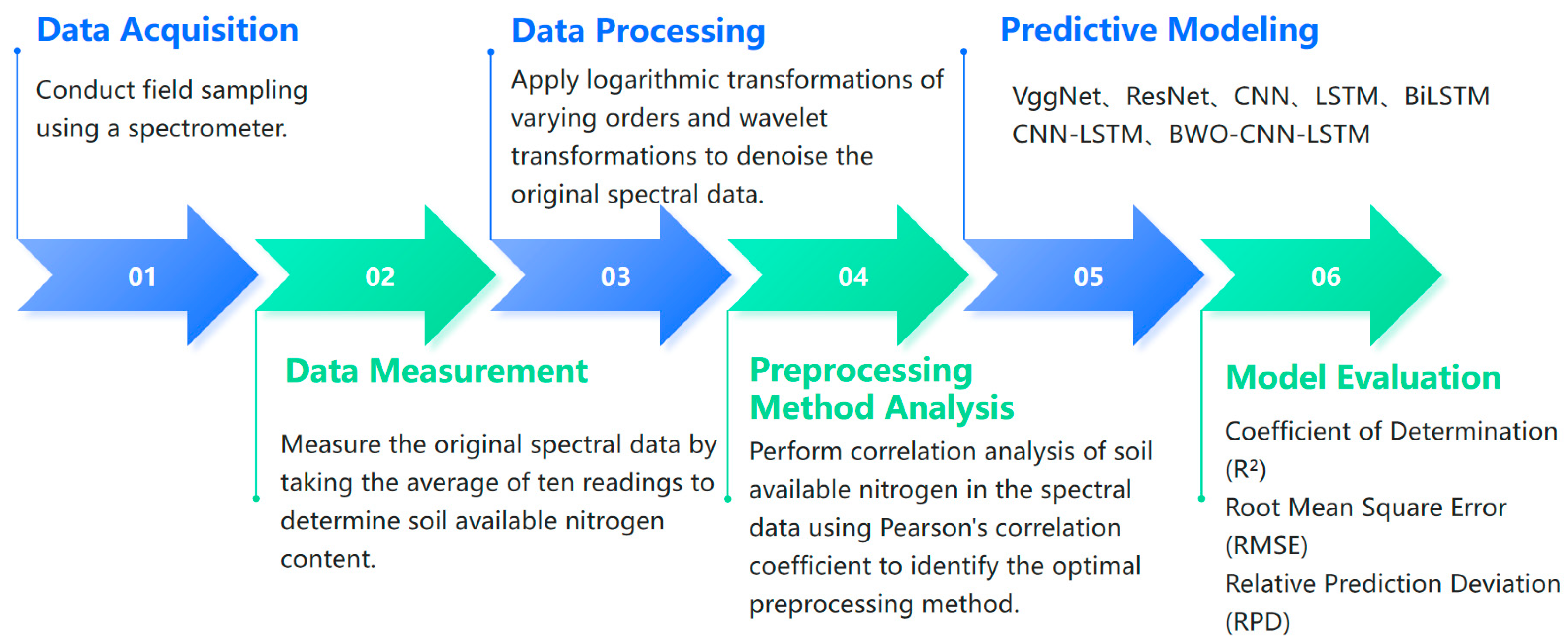
In this study, at first, the raw soil spectral data were preprocessed using three mathematical transformation methods: raw data (R), various logarithmic differential transformations (LOG), and wavelet transformation (WT). A total of 28 experiments were conducted, comparing and analyzing the differences in absorption characteristics, band overlap, and the magnitude of spectral peaks and troughs under different logarithmic differential transformations. A correlation analysis was then performed for each preprocessing method. Subsequently, seven deep learning modeling methods were tested, including VggNet, ResNet, CNN, LSTM, BiLSTM, CNN-LSTM, and BWO-CNN-LSTM. The prediction accuracy of available nitrogen content was compared across these models, and the optimal preprocessing method and modeling approach were selected. The experimental process for soil available nitrogen determination is shown in Figure 2.

2.4. Spectral Processing Methods

2.4.1. SPXY Sample Partitioning Algorithm

The SPXY algorithm optimizes the Kennard-Stone algorithm [18] and demonstrates greater scientific and practical utility when handling spectral data for soil available nitrogen content. While the traditional Kennard-Stone algorithm primarily divides samples based on spatial distribution, the SPXY algorithm considers both the spectral data characteristics and the distribution of soil available nitrogen content at the same time. Its core lies in the distance formula, which not only accounts for spatial distance but also incorporates spectral data variation and changes in available nitrogen content. The algorithm identifies a highly representative and evenly distributed subset of samples by calculating a distance matrix and selecting the most distant samples iteratively. It makes the SPXY algorithm more scientific and effective in sample partitioning, resulting in more reasonable sample selection.

2.4.2. Logarithmic Differential Transformation (LOG)

Research has shown that applying a first-order differential transformation for the raw spectral data can enhance spectral differences and reduce spectral loss [19]. However, a potential drawback is maybe missing that the optimal solution. To enhance internal spectral differences more precisely, a logarithmic differential transformation is employed in this study to process the spectra. The logarithmic differential calculation method is shown in Equation (1):
The formula for the oth derivative in the interval [a, b] is as follows:
d o f θ = lim h 0 1 h o m = 0 b a / h 1 m Γ o + 1 m ! Γ o m 1 f θ m h
Here, h represents the equidistant sampling step size, a is the starting point of the spectral segment, m is the summation index, Γ(·) is the Gamma function, and the coefficients of the above formula are the generalized binomial coefficients of the real number order σ. This expression essentially performs a weighted finite difference on the function values of each sampling point to the left of θ with power-law decays weights, and converges to a σ -order derivative when h→0, thereby extending the traditional integer order derivative that only depends on the local neighborhood to any positive real number order. When σ∈N, it degenerates into regular first, second, and other derivatives. Applying this operation to the logarithmic transformed spectral g(θ) can compress the dynamic range; convert multiplicative disturbances into additive terms; and while suppressing baseline drift and peak overlap, enhance the narrow and weak absorption characteristics, thereby more precisely characterizing the internal spectral difference. Given that excessively high orders may amplify noise, in actual modeling, the optimal σ is selected by combining wavelet denoising and validation set metrics to avoid excessive enhancement.
In this study, the power of the logarithmic differential was varied in intervals of 1, with the logarithmic base ranging from 5 to 20, forming a logarithmic differential transformation that varies from log10(5) to log10(20). When the values are log10(5) and log10(10), which represent the raw, unprocessed reflectance spectra and the reflectance spectra processed by first-order differential transformation, respectively.

2.4.3. Wavelet Transformation (WT) for Noise Reduction

Wavelet transformation denoising is a method that employs wavelet functions to decompose signals across multiple scales, extracting useful information from various frequency bands effectively to reduce noise interference in hyperspectral data [20]. The threshold denoising method based on wavelet transformation proposed by Donoho [21], was applied in this study.

2.5. The Structure of the BWO-CNN-LSTM Network

The Beluga optimization algorithm is used to optimize the hyperparameters of the CNN-LSTM model to improve the model’s predictive performance. The optimization process includes the following steps:
(1) Determine the set of hyperparameters required for the model, including the number and size of convolution kernels in the convolutional neural network, the number of hidden layer neurons in the long short-term memory network, and the learning rate of the model.
(2) Establish an evaluation criterion for model performance. The root mean square error of the validation set is used as the fitness function to evaluate the prediction accuracy of the model under each set of parameter configurations. During the optimization process, the Beluga optimization algorithm simulates the intelligent foraging behavior of the beluga group and performs a global search in the parameter space. In the early stage of the algorithm, a large search step size is used for extensive exploration, and the search range is gradually narrowed as the iteration proceeds. At the same time, the algorithm effectively avoids the optimization process from falling into the local optimal solution by introducing a random perturbation strategy. After multiple rounds of iterations, the algorithm finally outputs the optimal parameter combination that minimizes the validation set error.
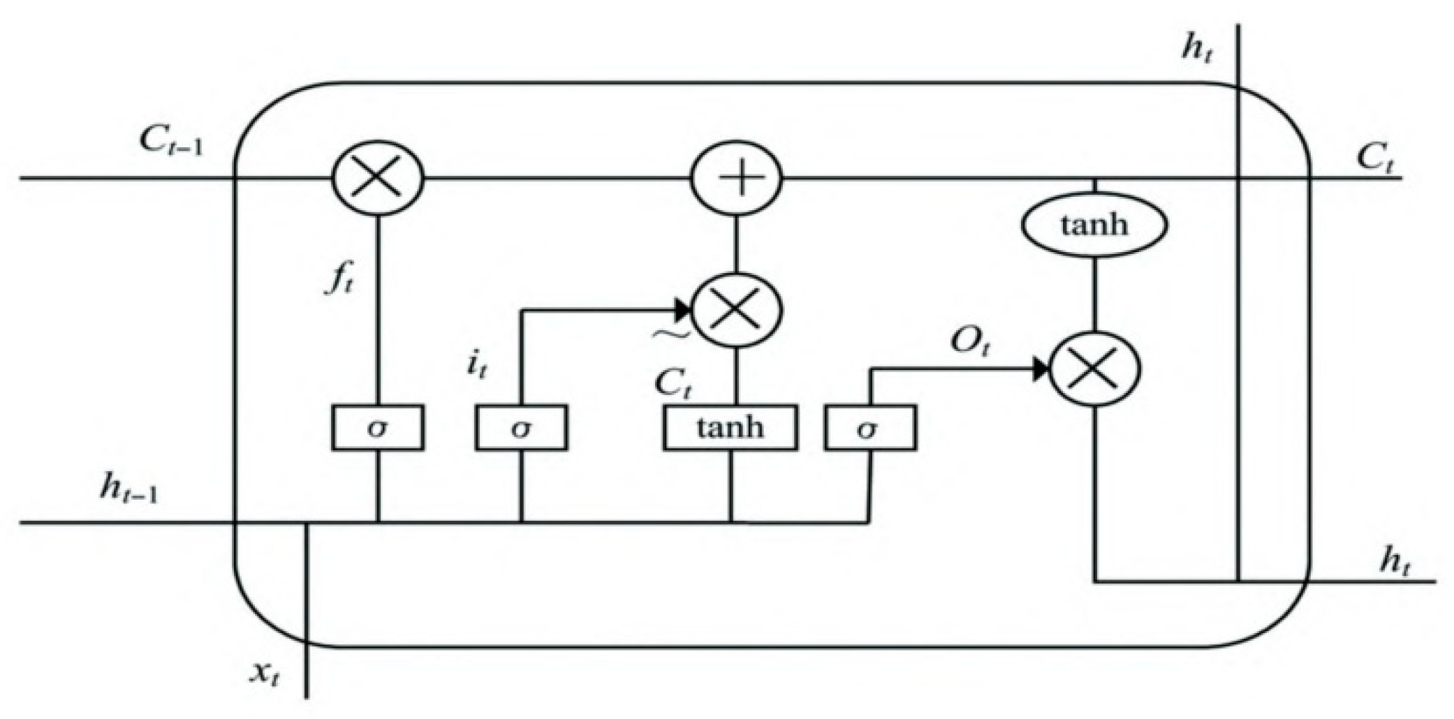
The LSTM network model contains three gates: the input gate, forget gate, and output gate, as illustrated in Figure 3. These gates allow the LSTM to effectively control and manage the cell state within the network. Through the gating mechanism, LSTM networks can capture long-term dependencies in sequential data, improving model accuracy and mitigating the vanishing gradient problem. The unique gating design is used for flexible decisions on which information to forget and which to retain. The input gate determines which new information should be added to the cell state. This process occurs in two steps: first, the sigmoid layer of the input gate decides which values to update, and second, the tanh layer generates a candidate vector to added to the cell state. The input gate state update formula is as follows:
i t = σ W i h t 1 , x t + b i
C t ~ = tanh W c h t 1 , x t + b c
In Equations (2) and (3), σ ( ) represents the sigmoid function, x t denotes the vector formed by the output of the LSTM at the previous time step and the input to the LSTM at the current time step, i t is the output of the input gate, W i is the weight matrix of the input gate, and b i is the bias of the input gate. C t ~ represents the cell state at the current time step, W c is the weight of the input unit, and b c is the bias of the input unit.
The forget gate is a sigmoid layer that integrates the hidden state from the previous time step and the current input data to decide whether the information is allowed to pass through. A value of “0” indicates complete forgetting, while “1” indicates complete retention. The state update formula for the forget gate is as follows:
f t = σ W f h t 1 , x t + b f
In Equation (4), f t represents the output of the forget gate, W f is the weight matrix of the forget gate, and b f is the bias of the forget gate.
The output gate determines the output information based on the current cell state. First, a tanh layer is applied to map the cell state to the range (−1, 1). Then, the sigmoid layer of the output gate controls which part of the cell state information is passed as output. The state update formula for the output gate is as follows:
o t = σ W o h t 1 , x t + b o
In Equation (5), o t represents the output of the current output gate, W o is the weight matrix of the output gate, and b o is the bias of the output gate.
The update for the cell state is as follows:
C t = f t C t 1 + i t C t ~
In Equation (6), represents the Hadamard product.
The output is as follows:
h t = o t tanh C t
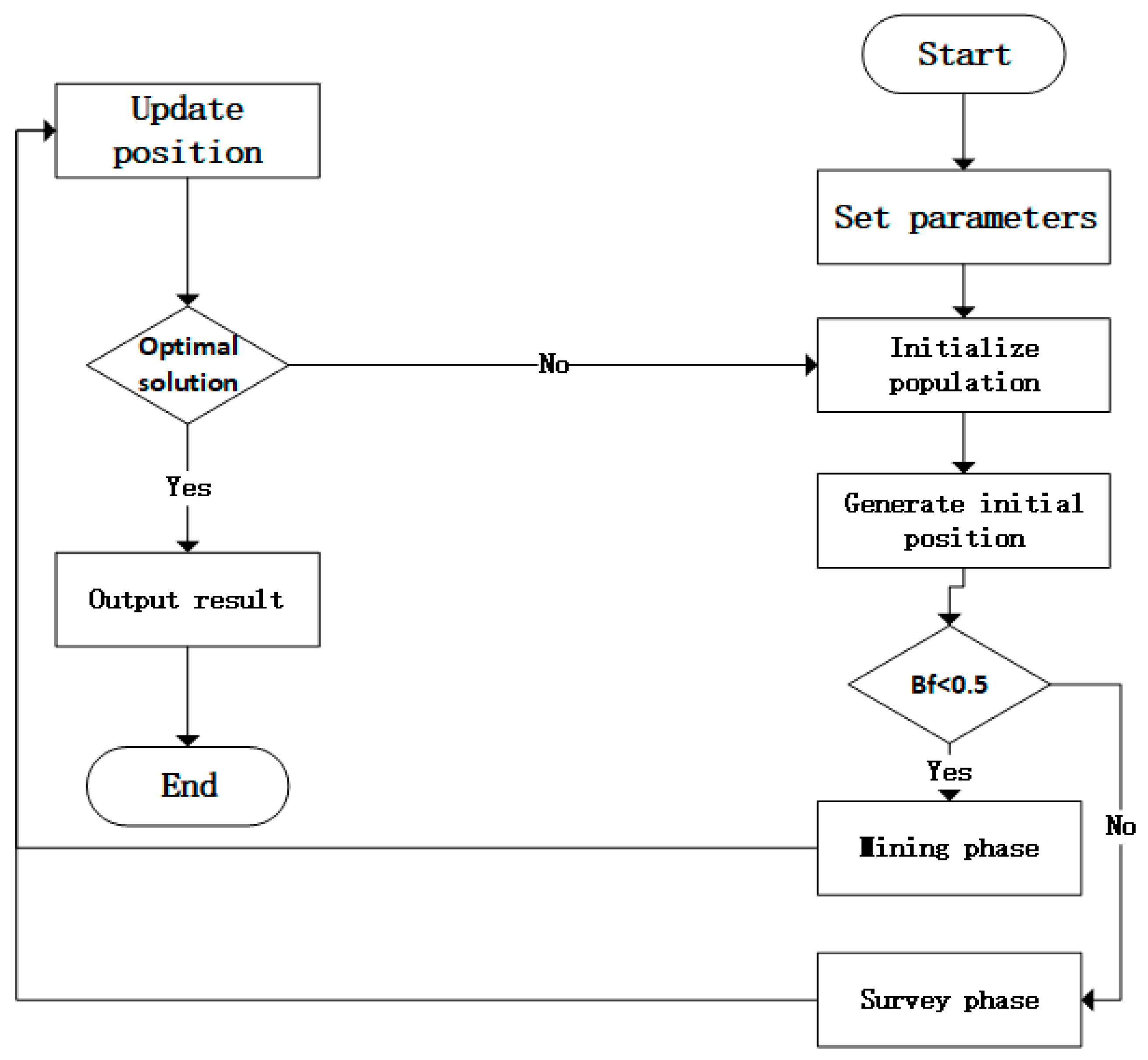
The convergence characteristics of the Beluga Optimization Algorithm (BWO) [22] are as follows: the probability of whale falling decreases linearly from 0.1 in the initial iteration to 0.05 in the final iteration. This dynamic adjustment mechanism reflects the evolutionary trend that as the optimization process progresses, the individual convergence risk gradually decreases, which is more conducive to gathering in the optimal solution area. The theoretical framework of the algorithm contains three core operation operators: a global exploration operator based on swimming behavior; a local development operator that simulates predation behavior; and a population update mechanism inspired by the natural falling phenomenon. The process and steps of the BWO are shown in Figure 4.
Step 1: Set the population size n and the maximum number of iterations Tmax, randomly generate the initial population and evaluate the fitness
Step 2: Dynamically adjust the search strategy according to the value of the balance factor Bf (Bf > 0.5 for exploration, Bf ≤ 0.5 for development), update the individual position and re-evaluate the fitness
Step 3: Calculate the falling probability Wf of the current iteration.
Step 4: Terminate the algorithm when the number of iterations exceeds Tmax, otherwise continue to execute the optimization loop.
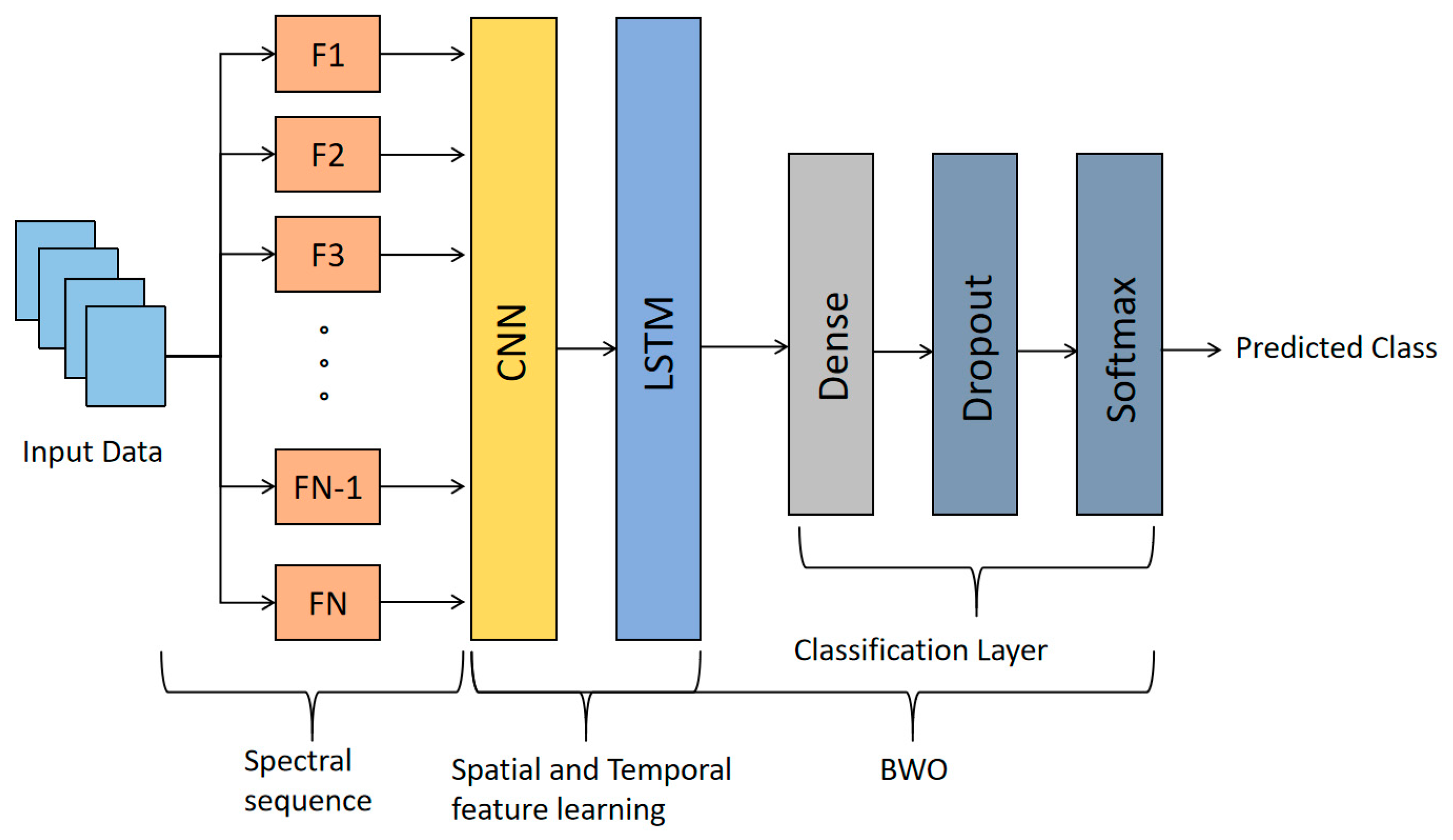
The Beluga optimization algorithm significantly improves the parameter optimization efficiency of the CNN-LSTM model through intelligent search strategies. The algorithm simulates the intelligent behavior of beluga groups, dynamically balances global exploration and local development capabilities in the solution space, and enables the model to adaptively capture the multi-scale features of spectral data. The optimization process focuses on the convolution kernel parameters of CNN and the hidden layer structure of LSTM. Through iterative optimization, the feature extractor can more accurately identify local bands and global trends that are key to effective nitrogen prediction. The CNN-LSTM model optimized by BWO exhibits stronger feature selection capabilities: in the CNN stage, the optimized convolution layer can automatically enhance the extraction of effective spectral features; in the LSTM stage, the tuned network parameters significantly improve the sensitivity of time series modeling. This collaborative optimization mechanism enables the model to autonomously identify the spectral intervals that contribute most to the prediction while suppressing noise interference. The structural diagram of the BWO-CNN-LSTM model and the network layer parameters are shown in Figure 5 and Table 1, respectively.
The pseudocode for the proposed BWO-CNN-LSTM composite deep network structure is as following.
(1) Input Sequence data
(2) First Convolutional Layer
Conv1D (filters = 32, kernel_size = 3, activation = ‘relu’)
MaxPooling1D(pool_size = 2)
(3) Second Convolutional Layer
Conv1D (filters = 64, kernel_size = 3, activation = ‘relu’)
MaxPooling1D(pool_size = 2)
(4) Third Convolutional Layer
Conv1D (filters = 128, kernel_size = 3, activation = ‘relu’)
MaxPooling1D(pool_size = 2)
(5) First LSTM Layer
LSTM (units = 64, return_sequences = True)
(6) Second LSTM Layer
LSTM (units = 64)
(7) Flatten Layer
Flatten ()
(8) Dense Layers
Dense (units = 200, activation = ‘relu’)
Dropout (rate = 0.5)
Dense (units = 100, activation = ‘relu’)
Dropout(rate = 0.5)
(9) Output Layer
Dense (units = 1, activation = ‘sigmoid’)
(10) Compile the Model
Model.compile(optimizer = ‘adam’,
loss = ‘binary_crossentropy’, metrics = [‘accuracy’])
(11) Output: Prediction

2.6. Other Deep Learning Methods

2.6.1. VGGNet

VGGNet [23] (Visual Geometry Group Network) is a deep convolutional neural network architecture characterized with very deep network structure. It primarily utilizes multiple stacked 3 × 3 convolutional kernels and 2 × 2 max pooling layers for feature extraction. This design enables the network to capture intricate details in images while increasing both the depth and computational complexity of the network simultaneously.

2.6.2. ResNet

ResNet [24] (Residual Network) was developed to address the degradation problem encountered in training deep neural networks. Its core concept is the introduction of residual blocks, which incorporate Skip Connections that allow the input to be able to propagate to the output directly. This approach mitigates issues related to gradient vanishing and gradient explosion effectively, enabling the training of much deeper models.

2.7. Evaluation Metrics

To reasonable evaluate the modeling capability of the BWO-CNN-LSTM, three performance metrics are employed:
R2 (R-squared): R2 is a regression model evaluation metric used to measure the degree to which the model explains the variance of the observed data. Its value ranges from 0 to 1, with values closer to 1 indicating a higher level of model fit to the data, while values approaching 0 suggest poor fitting. R2 is value of 1, and indicates perfect model fitting, whereas a value of 0 implies that the model fails to explain the variance in the data. The formula is as follows:
R 2 = 1 i = 1 n y i y ^ i 2 i = 1 n y i y ¯ 2
RMSE (Root Mean Squared Error): RMSE measures the prediction error of the model on continuous variables by calculating the root mean square of the differences between observed values and model predictions. Less RMSE indicates greater accuracy in the model’s predictions of observed values. The formula is as follows:
R M S E = 1 n i = 1 n y i y ^ i 2
PRD (Percentage Relative Difference): PRD assesses the relative error between predicted values and observed values, representing the difference between predicted and observed values as a percentage of the observed value. A less PRD signifies that the model’s predictions are closer to the true values. The formula is as follows:
R P D = S D R M S E

2.8. Experimental Environment

This study was conducted in an environment equipped with Windows 10, an NVIDIA GeForce RTX 3060 GPU, and 16 GB of RAM. The models, including VGGNet, ResNet, CNN, LSTM, BiLSTM, CNN-LSTM, and BWO-CNN-LSTM, were designed and implemented using Python 3.10 in conjunction with TensorFlow 2.13.0, with PyCharm 2024.1.1 serving as the integrated development environment (IDE).

3. Results

3.1. Statistical Characteristics of Soil Available Nitrogen Content

The SPXY algorithm was employed to partition 196 soil samples with varying levels of available nitrogen content, creating training and validation datasets at a 4:1 ratio to ensure an even and representative distribution of data. A total of 157 samples were designated for model training, while 39 samples were utilized to assess the model’s predictive performance. As shown in Table 2, the available nitrogen content across the 196 samples from the study area exhibited a wide range, fluctuating from a minimum (30.9 g/kg) to a maximum (399.7 g/kg), with a stable mean of 118.11 g/kg and a standard deviation of 60.37, indicating a moderate variation of 51.11%. The kurtosis value suggests a relatively peaked data distribution, while the skewness value indicates the asymmetry of the distribution.
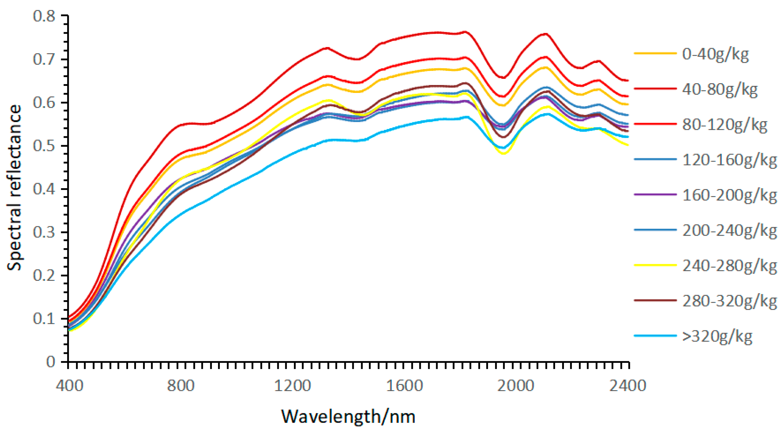
The available nitrogen content was categorized into groups with intervals of 40 g/kg, and the mean spectral reflectance for each group was calculated. As illustrated in Figure 6, the spectral reflectance curves for the different sample groups exhibited similar trends. In the 400–1320 nm wavelength range, the spectral reflectance increased with rising wavelengths significantly, demonstrating a very steep upward trend. Between 1320 and 2100 nm, the spectral reflectance stabilized with minimal fluctuations. However, in the 2100–2400 nm range, a downward trend in spectral reflectance was observed. Near 900 nm, the presence of an absorption peak related to iron oxide may influence the spectral reflectance.
The study also revealed a close relationship between available nitrogen content and spectral reflectance. Higher levels of available nitrogen generally corresponded to lower spectral reflectance, and vice versa.

3.2. Laboratory Spectral Preprocessing

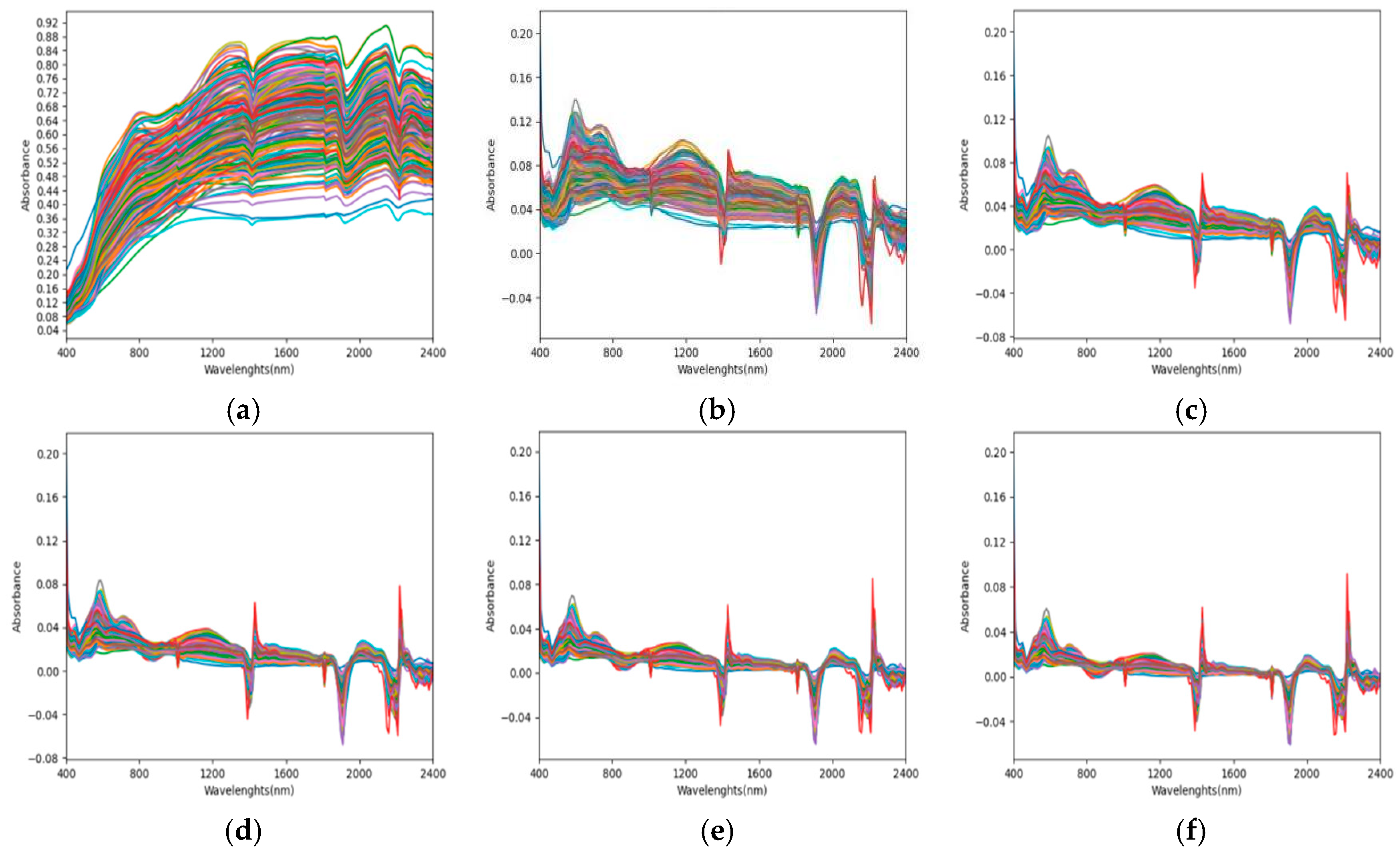
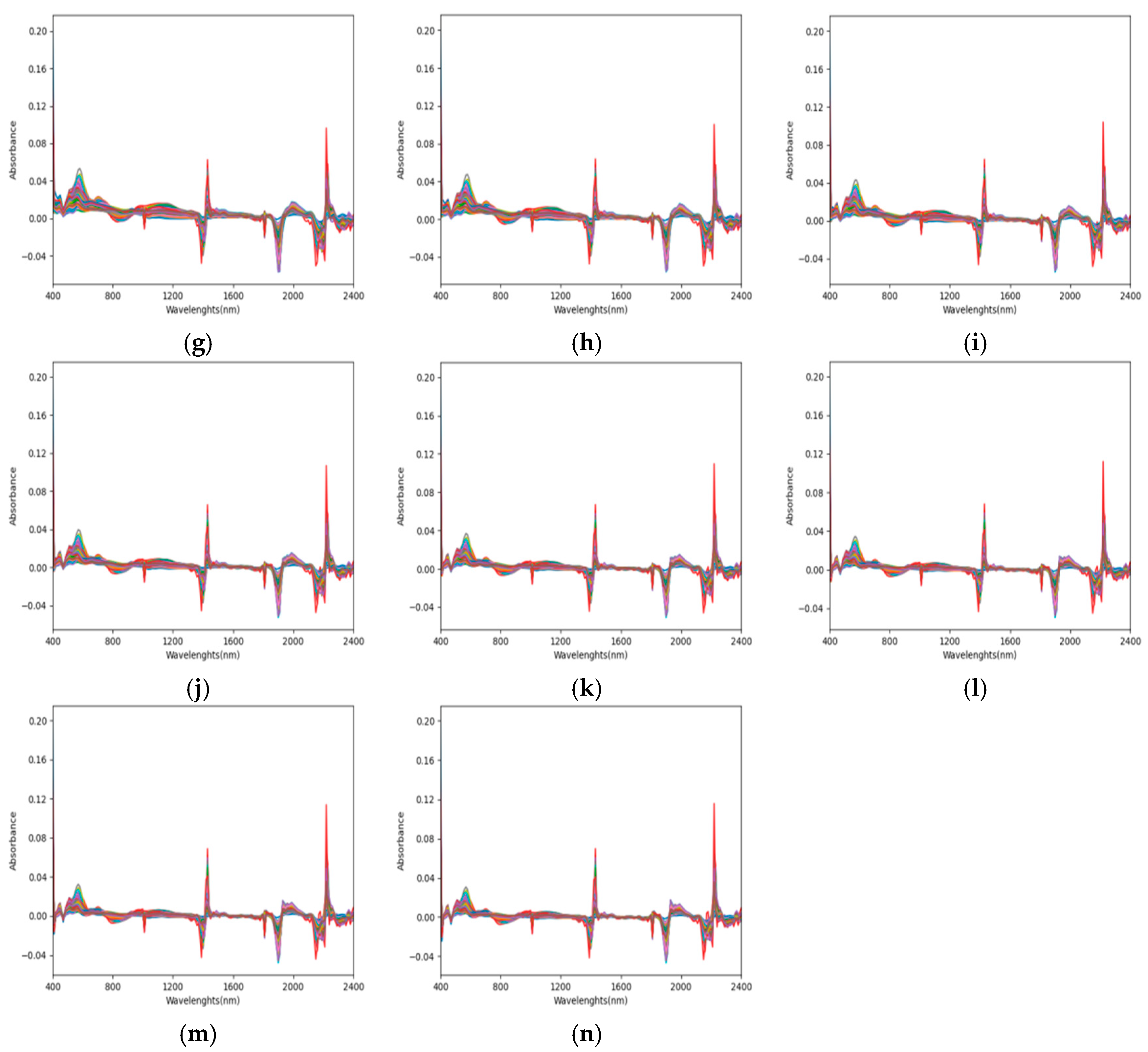
Spectral preprocessing is essential for enhancing feature extraction and model accuracy. The original spectral curves exhibit weak absorption features, band overlap, and broad reflectance ranges that obscure informative spectral content. To address these limitations, logarithmic differentiation (LOG) combined with wavelet transform (WT) was employed to strengthen the correlation between spectral parameters and soil nitrogen content.
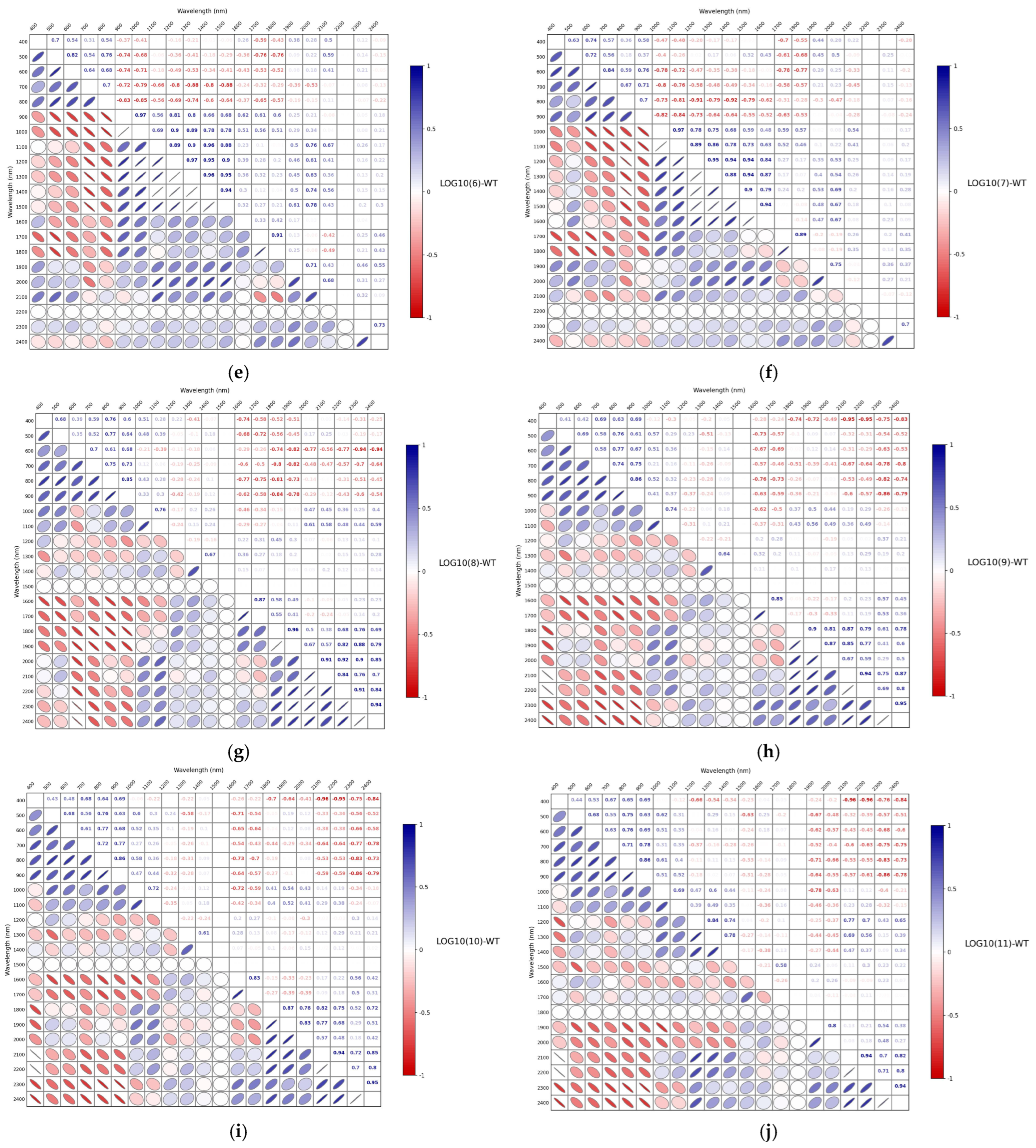
Systematic evaluation of LOG orders from 3 to 15 (Figure 7) revealed that spectral characteristics evolve progressively with differentiation order. Lower orders (LOG10(3)–LOG10(5)) show minimal changes in absorption features, while moderate orders (LOG10(6)–LOG10(9)) progressively mitigate peak overlap and baseline drift as reflectance values approach zero. At LOG order 10, optimal information extraction is achieved with most reflectance near zero and reduced curve fluctuations. Beyond LOG10(10), excessive differentiation leads to information loss, amplified noise, and diminished diagnostic absorption features. Based on this analysis, LOG10(10) was selected as the optimal preprocessing order, effectively capturing latent spectral information while preserving signal integrity for subsequent modeling.

3.3. Correlation Analysis of Spectra After Different Mathematical Transformations

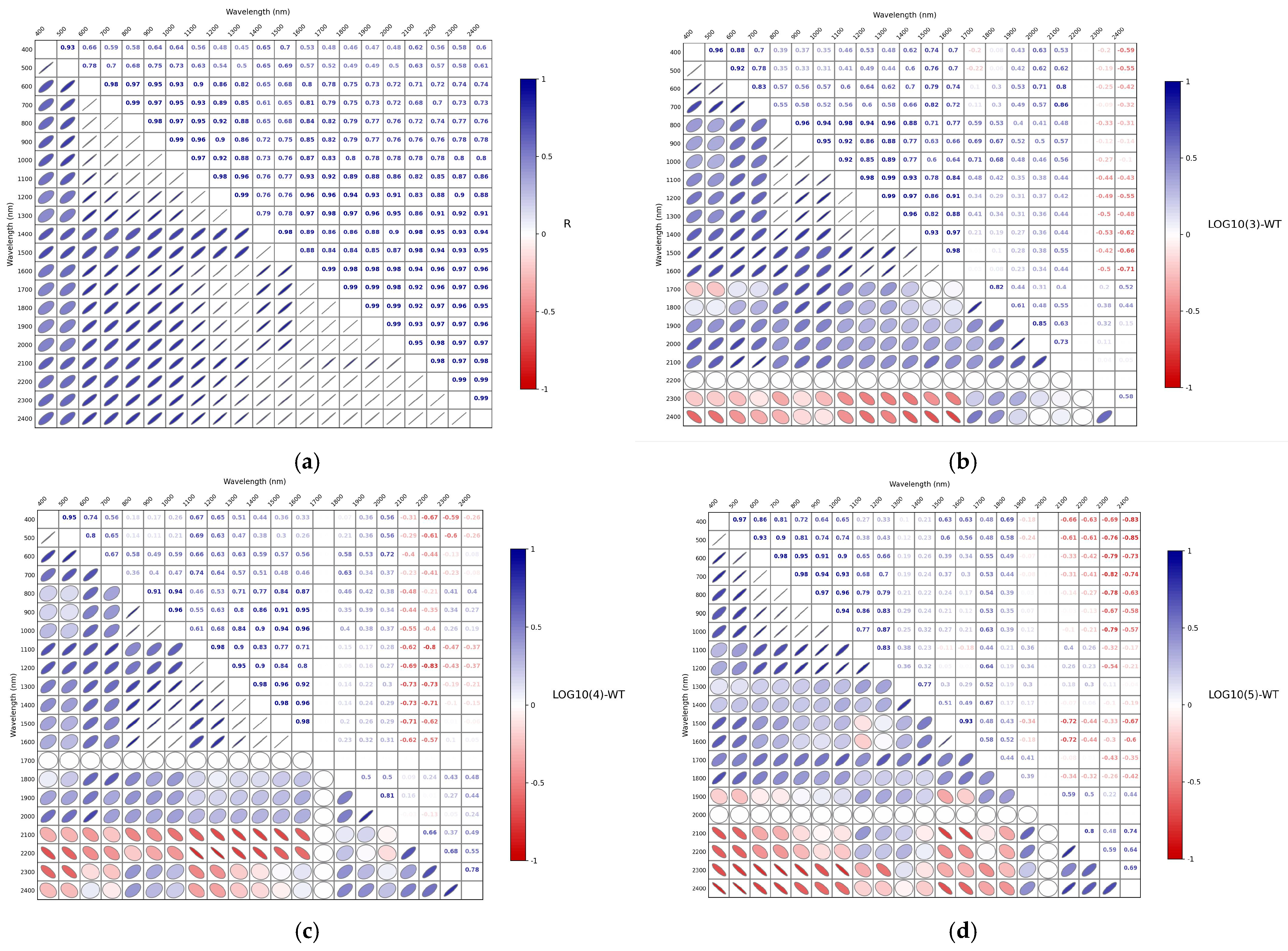
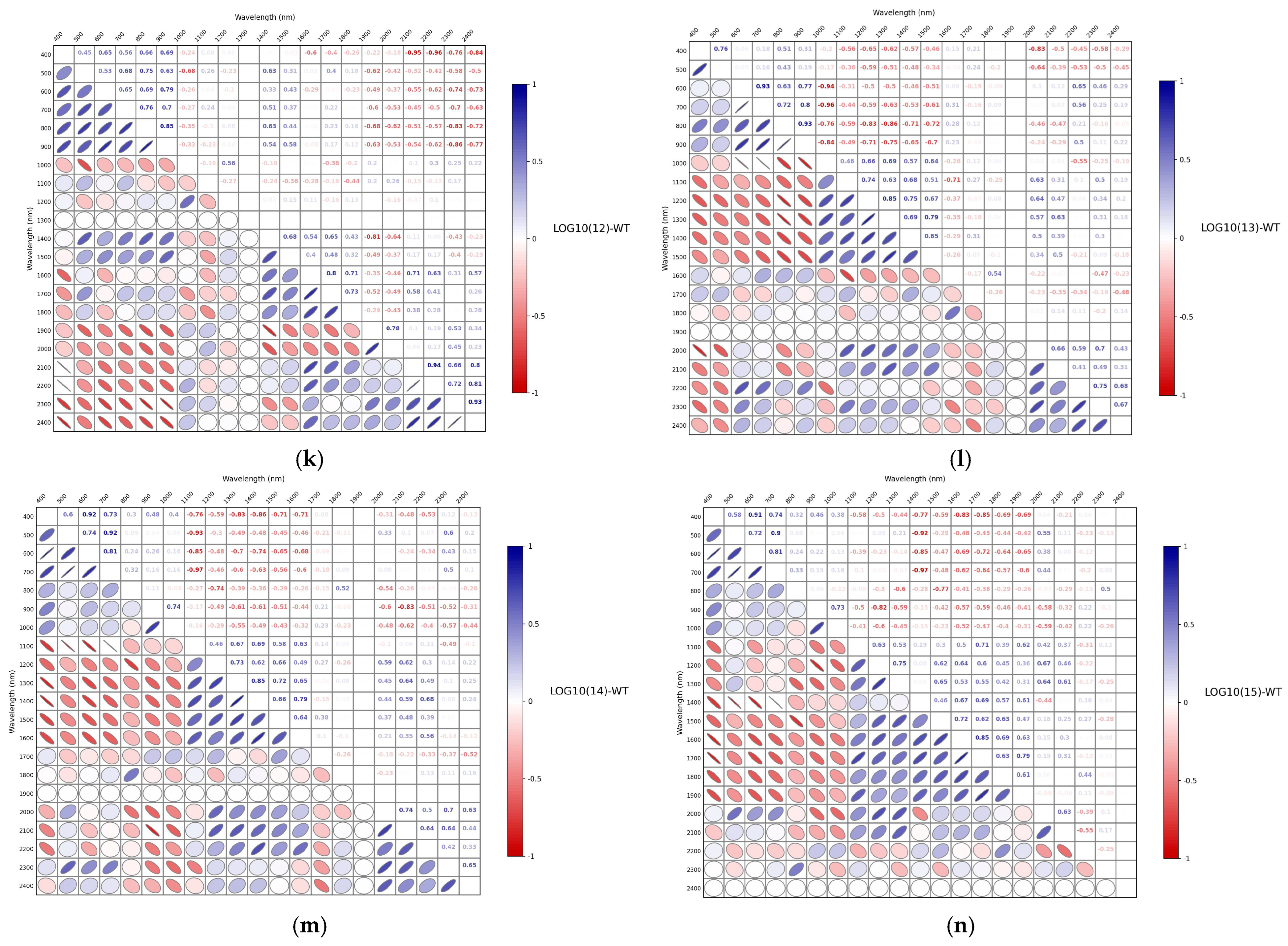
In Section 3.2, the application of logarithmic differentiation transformation for detecting and amplifying feature band information was elucidated. As illustrated in Figure 8a, the reflectance of the original spectral data and the content of available nitrogen exhibit an overall positive correlation. Figure 8b–n analyzes the spectral correlation coefficient heat maps of available nitrogen in soil processed with different powers of LOG combined with wavelet transformation (WT). The closer shapes are to a circle, the nearer correlation coefficients are to zero, with colors approaching white; red indicates negative correlation, and blue signifies positive correlation. The deep blue regions between 600 nm and 1500 nm indicate strong correlations, with absolute values of the correlation coefficients generally exceeding 0.7, peaking at a maximum coefficient of 0.99 in the 600 nm to 700 nm range. The white circles that appear at the beginning of 2200 nm in the figure signify a decline in the correlation coefficients within the spectral range. As shown in Figure 8c–n, with increasing powers of logarithmic differentiation, the correlation coefficients undergo continual changes, gradually revealing both positive and negative correlations. The heat map transitions are from a uniform blue to a distinctly layered array of colors; as the fractional order increases, the spectral reflectance approaches zero, and the corresponding colors in the correlation heat map begin to turn white.
The heat map for first-order differentiation exhibits fewer red and blue colors compared to those for LOG10(9), LOG10(13), and LOG10(14), and indicates that first-order differentiation lacks sensitivity to the gradual inclines present in the original reflectance, thereby overlooking effective information within the spectra. Conversely, logarithmic differentiation, with its incremental adjustments, processes the spectral information more accurately, ensuring a gradual change in the signal-to-noise ratio while extracting as much sensitive information as possible from the spectral curves. Because fold-wise validation scores are not independent due to substantial training set overlap between cross-validation folds, we refrain from applying parametric significance tests on cross-validated metrics and instead focus on effect sizes and interval estimates, following recommendations for model comparison under resampling. Conventional paired tests violate independence assumptions and yield inflated Type I error rates under cross-validation conditions, potentially exceeding 50% rather than the nominal 5% level. Effect sizes are reported as percentage improvements, providing interpretable measures of practical improvement magnitude, while 95% confidence intervals computed via bias-corrected bootstrap resampling on pooled predictions quantify estimation uncertainty, with non-overlapping intervals indicating robust performance differences. This framework emphasizes practical significance and provides more reliable model comparison for cross-validated results.

3.4. VggNet Inversion Analysis Based on Different Preprocessing Methods

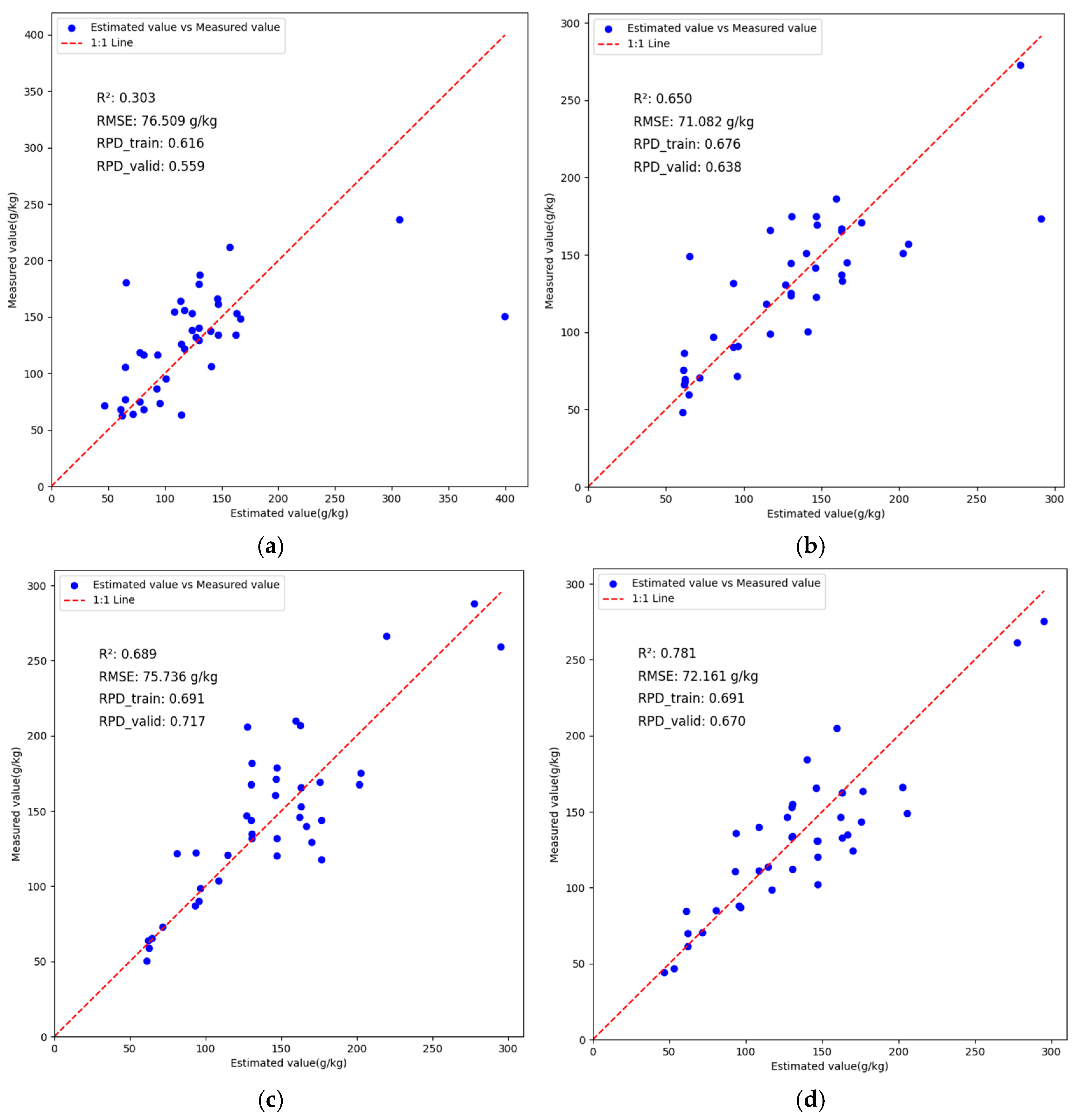
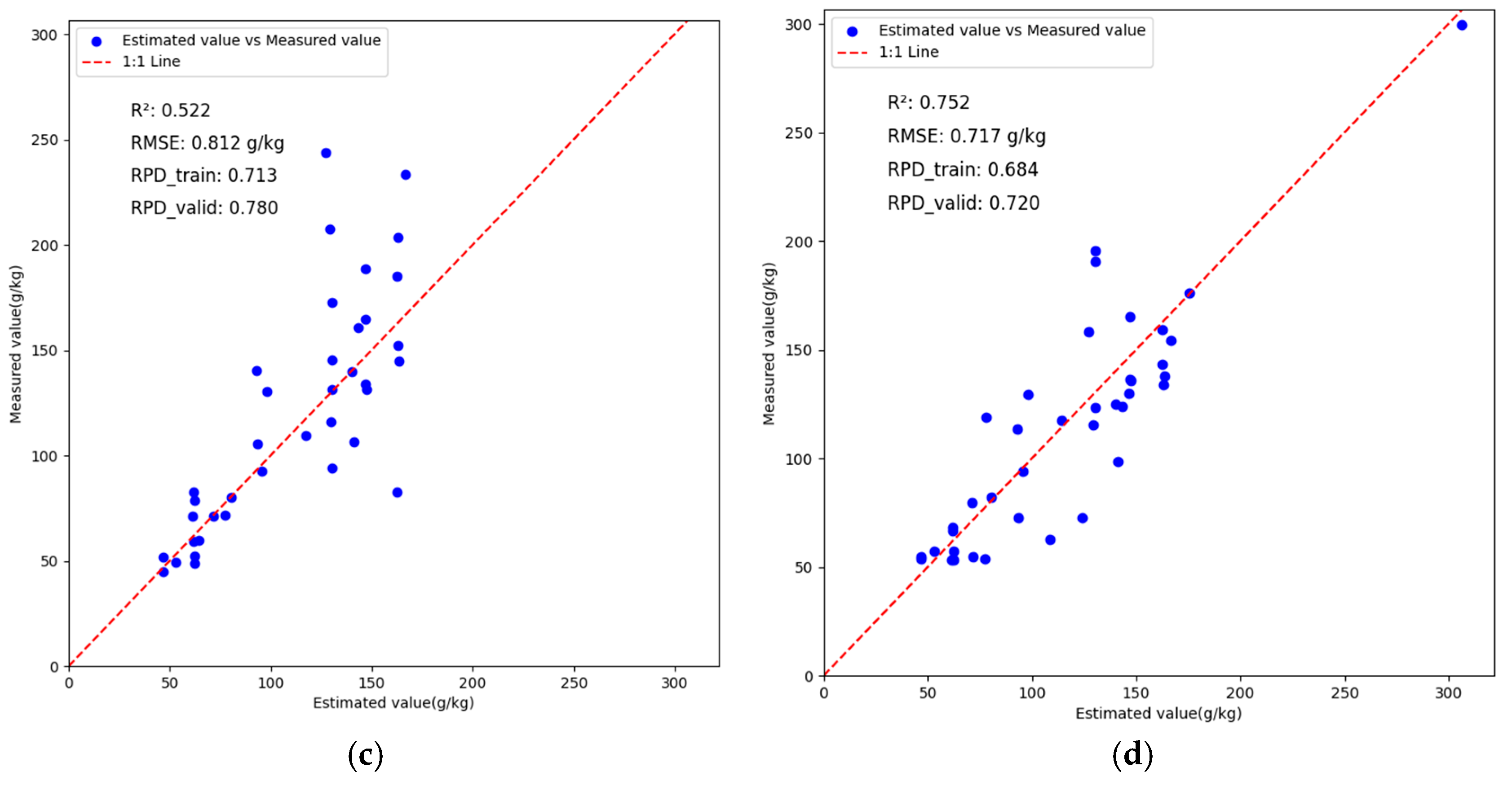
The VggNet regression modeling results based on different powers of logarithmic differentiation (LOG) combined with wavelet transformation (WT) are presented in Table 3. The R2 values for the validation set range from [0.3031 to 0.7811], with RMSE values ranging from [24.9976 to 52.8481] and RPD values ranging from [0.8087 to 1.9394]. Comparing the data in the table, it is evident that the VggNet model based on LOG10(9)-WT exhibits the best predictive accuracy, with validation set R2, RMSE, and PRD values of 0.7811, 24.9976, and 1.9338, respectively. Figure 9a–d depict scatter plots of measured versus predicted values, with the LOG10(9)-WT configuration being the closest to the 1:1 line. In contrast, the VggNet model based on LOG10(10)-WT yields validation set R2, RMSE, and PRD values of 0.6894, 29.3535, and 1.8491, respectively. Moreover, the performance of the VggNet model based on LOG + WT consistently surpasses that of the first-order differentiation model in terms of predictive accuracy. In summary, the fitting effectiveness of the LOG + WT algorithm within the VggNet deep learning model demonstrates significant improvement compared to first-order differentiation combined with WT.

3.5. ResNet Inversion Analysis Based on Different Preprocessing Methods

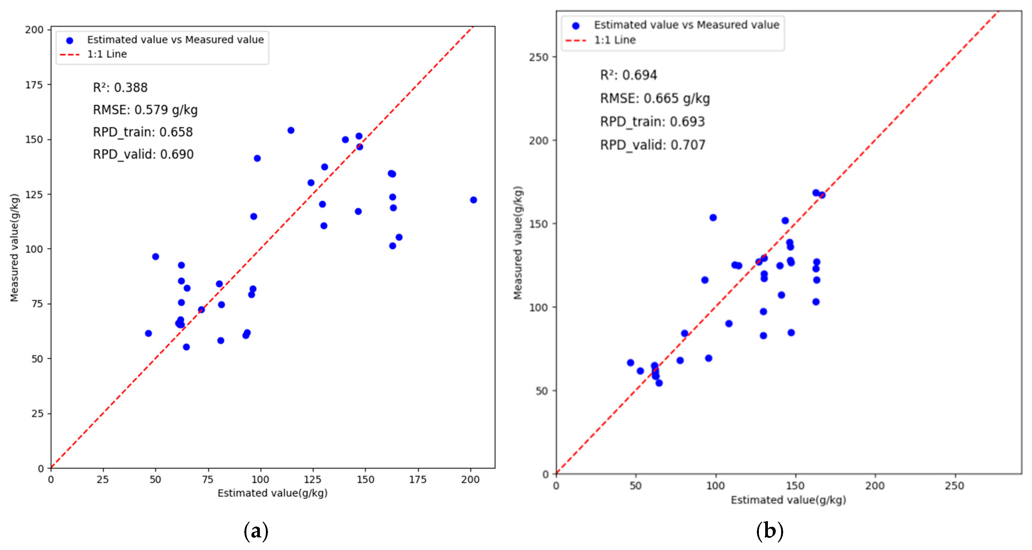
The modeling results of the ResNet network based on the combined preprocessing method of logarithmic differentiation (LOG) and wavelet transformation (WT) with different powers are presented in Table 4. It indicates that the coefficient of determination for the validation set ranges from 0.3882 to 0.7519, with mean squared error values ranging from 0.2475 to 0.3453, and relative percentage differences ranging from 1.2207 to 2.1209. After comprehensive comparison, the ResNet model based on LOG10(9)-WT demonstrated the best modeling performance, with validation set R2, RMSE, and PRD values of 0.7519, 0.2475, and 2.0846, respectively. In contrast, the ResNet model based on LOG10(10)-WT yielded validation set R2, RMSE, and PRD values of 0.5221, 0.3453, and 1.8356, respectively. Scatter plots of measured versus display predicted values in Figure 10a–d. The results indicate that, the ResNet model based on logarithmic differentiation (LOG) combined with WT exhibits superior accuracy and stability compared to the first-order differentiation (LOG10(10)) combined with WT within the deep learning framework of ResNet.

3.6. Analysis of BWO-CNN-LSTM Network Model Results

This study analyzes the impact of different powers of logarithmic differentiation (LOG) combined with Wavelet Transformation (WT) on model accuracy. The results demonstrate that the logarithmic differentiation with a power of 9, LOG10(9), combined with wavelet transformation is the optimal preprocessing method. Based on this foundation, CNN, LSTM, BiLSTM, and BWO-CNN-LSTM models were constructed and compared, with the experimental results presented in Table 5.
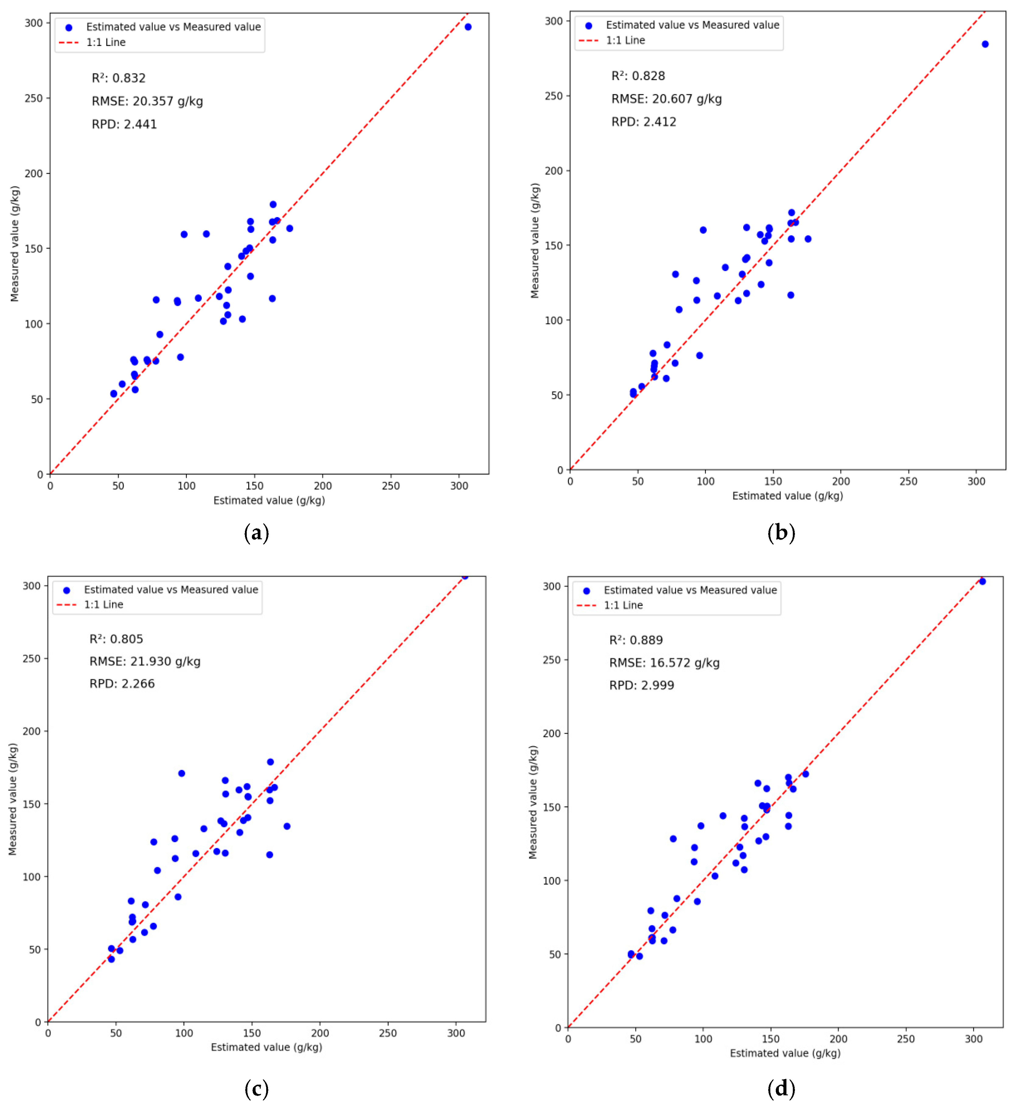
Seen from Table 5, the CNN model achieved an R2 of 0.9182, RMSE of 17.9361, and RPD of 3.4976 on the training set; on the validation set, it yielded an R2 of 0.8322, RMSE of 20.3567, and RPD of 2.4412. While CNN performed well on the training set, both R2 and RPD declined on the validation set. The LSTM model recorded an R2 of 0.8975, RMSE of 20.076, and RPD of 3.1247 on the training set; on the validation set, it achieved an R2 of 0.828, RMSE of 20.6073, and RPD of 2.4115. LSTM exhibited relatively stable performance on both sets, although overall metrics were inferior to those of CNN. The BiLSTM model showed an R2 of 0.8977, RMSE of 20.0609, and RPD of 3.1271 on the training set, with validation set metrics of R2 at 0.8052, RMSE at 21.9302, and RPD at 2.2661. BiLSTM’s performance on both datasets was similar to that of LSTM, though with slightly lower R2 and RPD values on the validation set. Compared with the CNN-LSTM model without BWO, the BWO-CNN-LSTM model improved R2 from 0.8569 to 0.8887 (an increase of 3.18%), RMSE from 18.2426 to 16.5722 (a decrease of 9.15%), and RPD from 2.7052 to 2.9987 (an increase of 10.85%) in the validation set. In contrast, the BWO-CNN-LSTM model achieved an R2 of 0.9403, RMSE of 15.3225, and RPD of 4.0941 on the training set; on the validation set, it reached an R2 of 0.8887, RMSE of 16.5722, and RPD of 2.9987. The BWO-CNN-LSTM model outperformed all other models on both datasets, with R2 and RPD on the test set increasing by 6.79% and 22.85%, respectively, and RMSE decreasing by 18.60% compared to CNN. When compared to LSTM, R2 and RPD on the test set improved by 7.34% and 24.34%, respectively, while RMSE decreased by 19.58%.
Scatter plots of measured versus predicted values is shown in Figure 11a–d. In summary, the BWO-CNN-LSTM model exhibits the excellent performance across all metrics and indicates its high accuracy in processing spectral data.

4. Discussion

This study demonstrates that the combination of a ninth-order logarithmic differential with a wavelet transform (LOG10(9) + WT) yields the best performance for estimating available soil nitrogen. Mechanistically, the logarithmic transform converts multiplicative noise and scale disparities into additive components while compressing dynamic range; the wavelet transform suppresses high-frequency noise across multiple scales and preserves narrowband features linked to molecular vibrations. On this basis, higher-order logarithmic differentiation further attenuates baseline drift and peak overlap, enhancing weak absorption edges and peak contrast. We observed that orders greater than 10 drive reflectance values toward zero and amplify noise, degrading effective information, whereas order 9 strikes a favorable balance between noise suppression and feature retention, consistent with diagnostic responses in the visible–near-infrared region (approximately 600–1500 nm).
At the model level, the superiority of the BWO–CNN–LSTM over CNN, LSTM, BiLSTM, and a non-optimized CNN–LSTM arises from the interplay of task-tailored architecture and unified global optimization. A 1-D CNN first extracts local band patterns and mitigates residual artifacts introduced by preprocessing; the LSTM then aggregates long-range dependencies along the wavelength axis to capture cross-band relations. Beluga Whale Optimization conducts a joint search over preprocessing parameters (LOG order, wavelet family/scale), architectural hyperparameters (kernel size and number, LSTM hidden units and layers, fusion and dropout), and training hyperparameters (learning rate, batch size, weight decay). The schedule combines early, large-step exploration with later exploitation and random perturbations to avoid local minima, improving convergence speed and solution stability. Under the same data and evaluation protocol, the proposed model achieved a validation R2 of 0.889, an RMSE of 16.5722, and a PRD of 2.9987 with low across-fold variance, indicating robust generalization.
Regarding generalizability, although the data originate from subtropical red-soil forests, the “preprocess–feature learning–sequence modeling–joint optimization” paradigm is transferable. The log-plus-wavelet combination provides broadly robust handling of multiplicative noise and background variation, and the CNN–LSTM division of labor between local and global spectral dependencies is not tied to a specific parent material. Nevertheless, differences among soil types, land uses, and climatic zones can shift optimal wavelength windows and preferred preprocessing orders. Practical transfer therefore benefits from retraining or fine-tuning on multi-site, multi-soil datasets, domain-adaptation or invariant-representation strategies, and hierarchical or clustered model ensembles to mitigate distribution shift.
In terms of computational cost and scalability, most overhead is incurred during the offline BWO search, which scales approximately with population size, number of iterations, and per-evaluation cost. Early stopping and proxy evaluations substantially shorten the search. Once the configuration is fixed, online inference requires a single forward pass and supports near-real-time prediction for thousands of spectra or streaming hyperspectral sequences. Additional pruning, knowledge distillation, and mixed-precision inference can further reduce latency and energy consumption without materially affecting accuracy, while the LOG + WT preprocessing can be batched or implemented as a streaming procedure at the sensor edge.
When compared qualitatively with recent benchmarks that combine hyperspectroscopy and deep learning, reported validation R2 values typically fall in the range of approximately 0.75–0.88, with RMSE dependent on units and scaling. Our performance lies at the upper end under comparable task definitions, though direct cross-study numerical comparisons should be interpreted cautiously because of differences in sample sizes, spectral coverage, experimental design, and evaluation protocols. To improve transparency, we summarize methods, datasets, and metrics under a consistent evaluation framework and emphasize effect sizes and interval estimates rather than relying solely on hypothesis tests.
Overall, LOG10(9) + WT achieves a favorable trade-off between noise suppression and information preservation, and the spectra-oriented, jointly optimized BWO–CNN–LSTM leverages complementary local and long-range spectral structure to deliver improved accuracy and stability for available nitrogen estimation in subtropical red-soil forests. Future work will extend validation to additional soil types and climates, develop domain-robust training strategies, and pursue compute-efficient optimization to further strengthen the method’s applicability to precision fertilization and sustainable soil management.
It is worth noting that we collected the spectra of the subtropical red soil forest plots in Guangxi under specific sensor Settings and preprocessing (LOG10(9) + WT). As a result, the learned representations may partly encode site-specific mineralogy (e.g., iron oxides), organic matter, moisture regime, texture, and canopy interference, as well as instrument response, and thus direct transfer to other soils and ecosystems should be undertaken with caution. In calcareous, volcanic, sandy, or highly organic soils, and in temperate or arid climates, baseline levels, absorption intensities, and noise structure can shift, potentially changing the optimal wavelength window and the effectiveness of the chosen preprocessing and hyperparameters. For operational deployment beyond subtropical red soils, we recommend external validation on independent sites, targeted recalibration or few-shot fine-tuning with locally sampled soils, and, where feasible, domain-adaptation strategies that promote spectral invariance across soil types and sensors; cross-instrument calibration and harmonized preprocessing are also advisable. Uncertainty quantification (e.g., prediction intervals) and soil-class-specific error reporting should accompany predictions to avoid over-confident decisions in management applications. These measures are essential to extend the method from its current, well-defined training context to broader agricultural and forestry settings while maintaining reliability.
The present study was conducted on a dataset of 196 forest soil samples in Guangxi. Although this dataset represents the soil diversity of the target area, the sample size is relatively limited compared with large-scale spectral studies. This constraint requires careful consideration of the potential impact of model generalization. The limited size of the dataset may impose some constraints on the model’s performance. The model’s ability to capture the full spectrum of soil variations in different ecological zones, parent materials and management practices may be limited, which may affect the prediction accuracy of soils whose features are not adequately represented in the training data. Secondly, small datasets increase the risk of overfitting. The model will learn sample-specific patterns rather than generalized spectral-nitrogen relationships. Moreover, the statistical ability to detect the subtle interaction between spectral features and soil properties may be reduced, which may limit the model’s robustness against environmental variability. However, judging from the results, our model still demonstrated good generalization ability and high accuracy, which also makes our conclusion reliable.
In conclusion, future work should address these limitations through strategic dataset expansion. Possible methods include: (1) assessing transferability by combining samples from neighboring provinces with similar climatic and geological conditions; (2) Spectral enhancement techniques such as noise injection, baseline correction variation or synthetic minority oversampling are adopted to artificially expand the training distribution; (3) Carry out targeted sampling activities in the underrepresented soil categories determined through uncertainty quantification; (4) Evaluate transfer learning methods, in which pre-trained spectral models from large public databases (such as LUCAS) are fine-tuned on regional data. These efforts will further verify the universality of the model and extend its applicability to a wider range of geographical environments, while maintaining the proven prediction accuracy.

5. Conclusions

This study used 196 soil samples from the Huangmian and Yachang state-owned forest farms in the Guangxi Zhuang Autonomous Region, China, to support model construction and to examine how spectral preprocessing affects performance across deep learning methods for hyperspectral prediction of available soil nitrogen. A comparative analysis was conducted under multiple preprocessing conditions.
(1) A spectral preprocessing scheme combining 9th-order logarithmic differentiation (LOG; LOG10(9)) with wavelet transform (WT) proved most effective. Relative to the original spectra, validation set R2 for VGGNet and ResNet increased by 0.478 and 0.3637, respectively; relative to the first-order derivative, the increases were 0.1314 and 0.0583. These results support LOG (order 9) + WT as the optimal preprocessing for this task.
(2) In the model comparison, the proposed BWO–CNN–LSTM outperformed CNN, LSTM, and BiLSTM, with validation set R2 increasing by 6.79%, 7.34%, and 10.37%, respectively; RMSE decreasing by 18.60%, 19.58%, and 24.44%; and PRD improving by 22.85%, 24.34%, and 32.30%. The convolutional feature extractor enhances LSTM sequence learning, and Beluga Whale Optimization improves parameter search and convergence, yielding superior predictive performance.
(3) The BWO–CNN–LSTM achieved validation set R2 = 0.889, RMSE = 16.5722, and PRD = 2.9987, enabling rapid and accurate prediction of available soil nitrogen in Guangxi forest lands. These results indicate practical value for precision nitrogen management and broader sustainable soil management by supporting timely monitoring and informed fertilization strategies.

Author Contributions

Conceptualization, Y.D. and C.L.; methodology, Y.C.; software, C.L.; validation, Y.D., Y.C. and C.L.; formal analysis, Y.C.; investigation, Y.D.; resources, C.L.; data curation, C.L.; writing—original draft preparation, Y.C.; writing—review and editing, Y.C.; visualization, Y.D.; supervision, Y.D.; project administration, Y.C.; funding acquisition, Y.D. All authors have read and agreed to the published version of the manuscript.

Funding

This study was funded by the Guangxi Key Research and Development Program (GuikeAB24010338, GuikeAB25069340), the National Natural Science Foundation of China (32360374), and the Innovation Project of Guangxi Graduate Education (YCSW2025405).

Institutional Review Board Statement

Not applicable.

Informed Consent Statement

Not applicable.

Data Availability Statement

Experimental data is available at https://github.com/lcsgsa-boop/cnn-lstm (accessed on 1 February 2025).

Acknowledgments

Here, we would like to express our gratitude to all the researchers who participated in the experiment for their efforts. Meanwhile, we also want to thank the institutions that have provided us with financial assistance. At the same time, we declare that we have not used any artificial intelligence tools to manipulate and generate any experimental data and results.

Conflicts of Interest

The authors declare no conflicts of interest.

References

  1. Wang, W.-C.; Yang, W.; Cui, Y.-L.; Zhou, P.; Wang, D.; Li, M.-Z. Prediction of soil total nitrogen content based on CatBoost algorithm and graph feature fusion. Trans. Chin. Soc. Agric. Mach. 2021, 52, 316–322. [Google Scholar]
  2. Zhang, Y.; Jian, J. Hyperspectral estimation modeling of soil As content in the eastern part of Tianfu New District, Chengdu based on SPA-BPNN. J. Guilin Univ. Technol. 2024, 44, 58–66. [Google Scholar]
  3. Zhong, H.; Li, X.-C. Indirect estimation of organic matter in cultivated soil based on surface soil spectrum. J. Anhui Agric. Univ. 2020, 47, 421–426. [Google Scholar] [CrossRef]
  4. Bremner, J.M. Nitrogen-total. Methods Soil Anal. 1996, 3, 1085–1121. [Google Scholar]
  5. Nocita, M.; Stevens, A.; Noon, C.; van Wesemael, B. Prediction of soil organic carbon for different levels of soil moisture using Vis-NIR spectroscopy. Geoderma 2013, 199, 37–42. [Google Scholar] [CrossRef]
  6. Gholizadeh, A.; Borůvka, L.; Saberioon, M.; Vašát, R. Visible, near-infrared, and mid-infrared spectroscopy applications for soil assessment with emphasis on soil organic matter content and quality: State-of-the-art and key issues. Appl. Spectrosc. 2013, 67, 1349–1362. [Google Scholar] [CrossRef] [PubMed]
  7. Zhong, L.; Guo, X. Hyperspectral estimation of organic matter in red soil based on different convolutional neural network models. Trans. Chin. Soc. Agric. Eng. 2021, 37, 203–212. [Google Scholar]
  8. Liu, H.-J.; Zhang, B. Study on hyperspectral model of organic matter content in black soil. Acta Pedol. Sin. 2007, 1, 27–32. [Google Scholar]
  9. Liu, Z.-M.; Li, X.-Q. Inversion of total nitrogen content in rubber plantation soil in Yunnan based on hyperspectral analysis. Trop. Agric. Sci. Technol. 2023, 46, 35–41. [Google Scholar] [CrossRef]
  10. Yin, C.-Y.; Bai, Z.-J. Comparative study on soil total nitrogen content estimation models based on hyperspectral data. Soil Fertil. Sci. China 2022, 1, 9–15. [Google Scholar]
  11. Wang, L.-W.; Wei, Y.-X. Study on hyperspectral model of total nitrogen and total phosphorus content in wetland soil. Acta Ecol. Sin. 2016, 36, 5116–5125. [Google Scholar]
  12. Kim, S.; Choi, H.-J.; Park, S.; Kim, Y. Predicting the Freezing Characteristics of Organic Soils Using Laboratory Experiments and Machine Learning Models. Appl. Sci. 2025, 15, 10314. [Google Scholar] [CrossRef]
  13. Geng, W.; Li, T.; Zhu, X.; Dou, L.; Liu, Z.; Qian, K.; Ye, G.; Lin, K.; Li, B.; Ma, X.; et al. Predicting the Zinc Content in Rice from Farmland Using Machine Learning Models: Insights from Universal Geochemical Parameters. Appl. Sci. 2025, 15, 1273. [Google Scholar] [CrossRef]
  14. Alahmad, T.; Neményi, M.; Nyéki, A. Soil Moisture Content Prediction Using Gradient Boosting Regressor (GBR) Model: Soil-Specific Modeling with Five Depths. Appl. Sci. 2025, 15, 5889. [Google Scholar] [CrossRef]
  15. Ryu, S.; Kim, J.; Choi, H.; Lee, J.; Han, J. Case Study on Analysis of Soil Compression Index Prediction Performance Using Linear and Regularized Linear Machine Learning Models (In Korea). Appl. Sci. 2025, 15, 2757. [Google Scholar] [CrossRef]
  16. Zhong, A.-L.; Wang, X.-S. Quantitative modeling method of corn components based on near-infrared spectral fusion and deep learning. Food Ferment. Ind. 2020, 46, 213–219. [Google Scholar] [CrossRef]
  17. Zhang, D.-Y.; Wu, T.-J. Remote sensing fine mapping of agricultural planting structure based on spatiotemporal coordination. Natl. Remote Sens. Bull. 2024, 28, 2014–2029. [Google Scholar]
  18. Wu, Q.-Y.; Zhu, Z.-Y. Dataset representativeness measurement and block sampling strategy for the pan-Kennard-Stone algorithm. Chem. J. Chin. Univ. 2022, 43, 150–157. [Google Scholar]
  19. Zhang, Y.-L.; Wang, H. Estimation of soil organic matter content in mountainous cultivated land based on hyperspectral analysis. Jiangsu J. Agric. Sci. 2024, 40, 112–120. [Google Scholar]
  20. Hu, W.; Huang, Y. Deep convolutional neural networks for hyperspectral image classification. J. Sens. 2015, 2015, 258619. [Google Scholar] [CrossRef]
  21. Donoho, D.L.; Johnstone, I.M. Ideal spatial adaptation by wavelet shrinkage. Biometrika 1994, 81, 425–455. [Google Scholar] [CrossRef]
  22. Zhong, C.; Li, G.; Meng, Z. Beluga whale optimization: A novel nature-inspired metaheuristic algorithm. Knowl.-Based Syst. 2022, 251, 109215. [Google Scholar] [CrossRef]
  23. He, J.; Li, S.; Shen, J.; Liu, Y.; Wang, J.; Jin, P. Facial expression recognition based on VGGNet convolutional neural network. In Proceedings of the 2018 Chinese Automation Congress (CAC), Xi’an, China, 30 November–2 December 2018; IEEE: Piscataway, NJ, USA, 2018; pp. 4146–4151. [Google Scholar]
  24. Targ, S.; Almeida, D. Resnet in resnet: Generalizing residual architectures. arXiv 2016, arXiv:1603.08029 2016. [Google Scholar] [CrossRef]
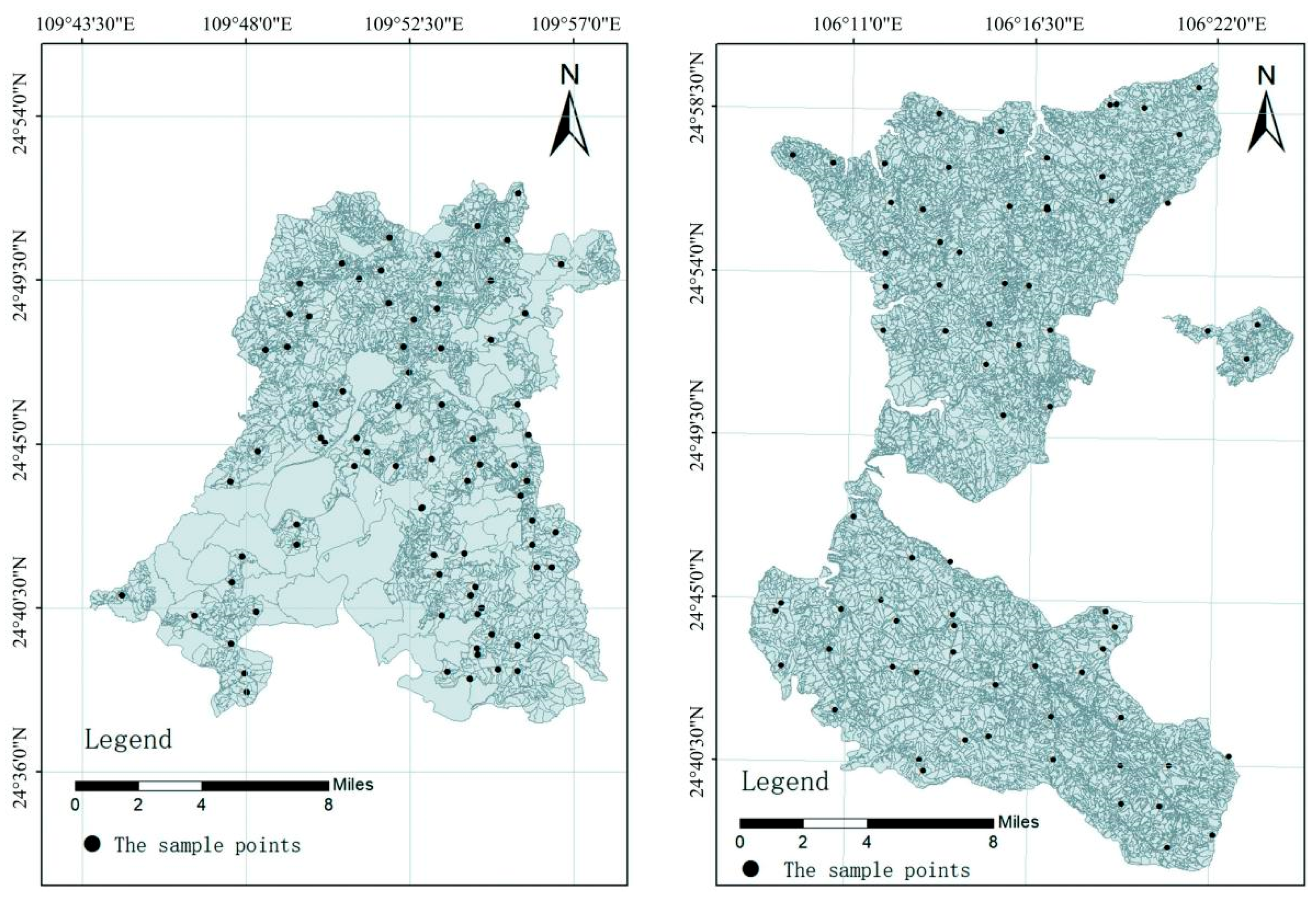
Figure 1. Soil Sample Collection Points.
Applsci 15 11077 g001
Figure 2. Flowchart of Soil Available Nitrogen Experimental Method.
Applsci 15 11077 g002
Figure 3. Long Short-Term Memory Network Structure.
Applsci 15 11077 g003
Figure 4. Beluga Optimization Algorithm Structure.
Applsci 15 11077 g004
Figure 5. BWO-CNN-LSTM Network Structure.
Applsci 15 11077 g005
Figure 6. Curves of Soil Samples with Different Available Nitrogen Content.
Applsci 15 11077 g006
Figure 7. (a) R. (b) LOG10(3) + WT. (c) LOG10(4) + WT. (d) LOG10(5) + WT. (e) LOG10(6) + WT. (f) LOG10(7) + WT. (g) LOG10(8) + WT. (h) LOG10(9) + WT. (i) LOG10(10) + WT. (j) LOG10(11) + WT. (k) LOG10(12) + WT. (l) LOG10(13) + WT. (m) LOG10(14) + WT. (n) LOG10(15) + WT.
Applsci 15 11077 g007aApplsci 15 11077 g007b
Figure 8. (a) R. (b) LOG10(3) + WT. (c) LOG10(4) + WT. (d) LOG10(5) + WT. (e) LOG10(6) + WT. (f) LOG10(7) + WT. (g) LOG10(8) + WT. (h) LOG10(9) + WT. (i) LOG10(10) + WT. (j) LOG10(11) + WT. (k) LOG10(12) + WT. (l) LOG10(13) + WT. (m) LOG10(14) + WT. (n) LOG10(15) + WT.
Applsci 15 11077 g008aApplsci 15 11077 g008bApplsci 15 11077 g008c
Figure 9. (a) R. (b) LOG10(10). (c) LOG10(10)-WT. (d) LOG10(9)-WT.
Applsci 15 11077 g009
Figure 10. (a) R. (b) LOG10(10). (c) LOG10(10)-WT. (d) LOG10(9)-WT.
Applsci 15 11077 g010aApplsci 15 11077 g010b
Figure 11. (a) CNN. (b) LSTM. (c) BiLSTM. (d) BWO-CNN-LSTM.
Applsci 15 11077 g011
Table 1. Parameters in BWO-CNN-LSTM Network.
Layer (Type)Output ShapeParameter
Conv1d(32, 128)128
Max_Pooling1d(32, 64)0
Conv1d_1(64, 64)6028
Max_Pooling1d_1(64, 32)0
Conv1d_2(128, 32)24,704
Max_Pooling1d_2(128, 16)0
Lstm6478,840
Lstm_16488,440
Flatten10240
Dense200322,200
Dropout1000
Activation10
Dense_110020,100
Dropout_1500
Dense_21101
Table 2. Statistical Characteristics of Soil Available Nitrogen Content.
Sample TypeSample SizeMinimum ValueMaximum ValueAverage ValueStandard DeviationKurtosisSkewnessCoefficient of Variation
All sample19630.9399.7118.1160.374.191.6051.11
Training
sample
15730.9396.1117.8057.703.821.5248.98
Validation
sample
3946.4399.7119.3069.824.231.7158.52
Table 3. VggNet Regression Modeling Results.
Preprocessing MethodTraining SetValidation Set
R2RMSERPDR2RMSERPD
R0.690633.12861.40810.303152.84810.8087
LOG10(10)0.915917.80333.170.649732.38121.4009
LOG10(3)-WT0.888119.76382.70360.438047.92290.9513
LOG10(4)-WT0.906219.25572.92120.708225.35661.8336
LOG10(5)-WT0.914818.05043.13930.756536.30671.9394
LOG10(6)-WT0.954513.29554.48360.673128.77391.7007
LOG10(7)-WT0.913516.67173.09130.452351.53790.8439
LOG10(8)-WT0.946814.61194.09030.668326.08861.7466
LOG10(9)-WT0.939215.11473.88060.781124.99761.9338
LOG10(10)-WT0.933315.69053.70590.689429.35351.8491
LOG10(11)-WT0.945214.23083.95130.739128.87471.7887
LOG10(12)-WT0.947213.94364.09960.761627.86311.7528
LOG10(13)-WT0.921916.99163.35690.655933.09861.4460
LOG10(14)-WT0.936515.17113.60110.708430.82131.5037
LOG10(15)-WT0.937515.06573.62810.747428.68781.7563
Table 4. ResNet Network Model Modeling Results.
Preprocessing MethodTraining SetValidation Set
R2RMSERPDR2RMSERPD
R0.85640.24212.30570.38820.32731.2207
LOG10(10)0.99250.054911.08780.69360.25591.8371
LOG10(3)-WT0.97540.09836.04570.56500.32751.6445
LOG10(4)-WT0.98740.07058.50570.58980.31351.3578
LOG10(5)-WT0.98280.08217.66160.58570.31911.7773
LOG10(6)-WT0.97730.09546.81820.65390.27131.9935
LOG10(7)-WT0.98550.076297.91310.71280.24991.9451
LOG10(8)-WT0.99030.06229.80160.68480.26412.1209
LOG10(9)-WT0.98410.0797.46820.75190.24752.0846
LOG10(10)-WT0.98840.06749.46810.52210.34531.8356
LOG10(11)-WT0.99320.051212.00390.67810.29441.9454
LOG10(12)-WT0.98590.07447.9730.61540.30691.471
LOG10(13)-WT0.98570.07497.92070.73870.25382.1009
LOG10(14)-WT0.99250.053911.27750.71910.26912.0034
LOG10(15)-WT0.99120.059510.5170.52980.32111.6004
Table 5. Modeling Results of CNN, LSTM, BiLSTM, and BWO-CNN-LSTM Models.
Preprocessing MethodTraining SetValidation Set
R2RMSERPDR2RMSERPD
CNN0.918217.93613.49760.832220.35672.4412
LSTM0.897520.0763.12470.82820.60732.4115
BiLSTM0.897720.06093.12710.805221.93022.2661
CNN-LSTM0.921716.99033.85750.856918.24262.7052
BWO-CNN-LSTM0.940315.32254.09410.888716.57222.9987
Disclaimer/Publisher’s Note: The statements, opinions and data contained in all publications are solely those of the individual author(s) and contributor(s) and not of MDPI and/or the editor(s). MDPI and/or the editor(s) disclaim responsibility for any injury to people or property resulting from any ideas, methods, instructions or products referred to in the content.