Article

Comparative Analysis and Validation of LSTM and GRU Models for Predicting Annual Mean Sea Level in the East Sea: A Case Study of Ulleungdo Island

1
Geodesy Laboratory, Civil & Architectural and Environmental System Engineering, Sungkyunkwan University, Suwon 16419, Gyeonggi, Republic of Korea
2
Disaster & Risk Management Laboratory, Interdisciplinary Program in Crisis & Disaster and Risk Management, Sungkyunkwan University, Suwon 16419, Gyeonggi, Republic of Korea
*
Author to whom correspondence should be addressed.
Appl. Sci. 2025, 15(20), 11067; https://doi.org/10.3390/app152011067 (registering DOI)
Submission received: 26 September 2025 / Revised: 6 October 2025 / Accepted: 6 October 2025 / Published: 15 October 2025

Abstract

This study presents a deep learning-based model for predicting annual mean sea level (MSL) in the East Sea, with a focus on the Ulleungdo Island region, which maintains an independent vertical datum. To account for long-term tidal variability, the model enables continuous estimation of hourly and annual MSL values. Two recurrent neural network (RNN) architectures—Long Short-Term Memory (LSTM) and Gated Recurrent Unit (GRU)—were constructed and compared. Observational tide gauge data from 1 January 2000 to 3 August 2018 (covering 18.6 years and a full tidal nodal cycle) were preprocessed through missing-value and outlier treatment, followed by min–max normalization, and then structured for sequential learning. Comparative analysis demonstrated that the GRU model slightly outperformed the LSTM model in predictive accuracy and training stability. As a result, the GRU model was selected to produce annual MSL forecasts for the period 2018–2021. The GRU achieved a mean RMSE of approximately 0.44 cm during this prediction period, indicating robust performance in forecasting hourly sea level variations. The findings highlight the potential of deep learning methods to support vertical datum determination in island regions and to provide reliable sea level estimates for integration into coastal and oceanographic modeling. The proposed approach offers a scalable framework for long-term sea level prediction under evolving geodetic conditions.

1. Introduction

Accurate prediction of mean sea level (MSL) is critical for addressing the challenges associated with sea level rise, improving the precision of vertical datum determination, and supporting various geodetic applications. In the Republic of Korea, several island regions are geographically isolated from the mainland, making it difficult to establish vertical datums through precise leveling connections. Traditionally, long-term tide gauge records have been used to estimate MSL; however, such approaches have limitations in fully capturing the nonlinear periodicity and long-term variability of sea level dynamics. To overcome these limitations, this study proposes a more reliable method for determining MSL by utilizing tide gauge observations spanning more than 18.6 years and applying a deep learning-based prediction model.

1.1. Motivation and Objectives

Accurate determination of mean sea level (MSL) is essential in geodetic applications, particularly for the realization of vertical datums. In practice, vertical datum definition relies on long-term tide gauge observations, which are used to establish a stable reference surface. However, conventional approaches that simply average extended observational records are limited in their ability to capture the inherent nonlinear periodicity of sea level variations, including those associated with the 18.6-year nodal factor cycle.
In the Republic of Korea, additional challenges arise in island regions that are geographically isolated from the mainland. Because precise leveling connections to national benchmarks cannot be performed in such areas, independent determination of vertical datums is required. This reliance on localized tide gauge data makes it necessary to explore advanced methods for estimating MSL with improved reliability and adaptability.
The objective of this study is to propose a deep learning-based prediction approach for MSL determination by utilizing tide gauge records spanning more than 18.6 years. Specifically, two recurrent neural network (RNN) architectures—Long Short-Term Memory (LSTM) and Gated Recurrent Unit (GRU)—were constructed and compared in terms of predictive accuracy and stability. Based on the comparative results, the more suitable model was applied to generate reliable MSL estimates for isolated island regions. The proposed approach is expected to complement traditional methods and contribute to more robust geodetic practices for vertical datum establishment.

1.2. Related Works

Recent advancements in deep learning (DL) have ushered in a new era of sea level prediction, enabling models to learn hierarchical features directly from data with improved accuracy, robustness, and generalizability. In particular, hybrid and ensemble deep learning architectures have demonstrated significant superiority over traditional approaches. Raj and Brown [1] developed a hybrid SVMD-CNN-BiLSTM model that integrates signal decomposition with convolutional and bidirectional LSTM layers and incorporates GNSS-derived VLM corrections. Their model achieved a correlation exceeding 0.95 and yielded accurate annual rise estimates, such as 4.5 mm/year at Port Kembla. Similarly, a stacked BiLSTM model using decomposed inputs and corrected observational data predicted MSL rise in vulnerable Pacific islands with correlations as high as 0.997 [2].
Ensemble models further enhance predictive performance through shared learning across spatial locations. Rus et al. [3] introduced HIDRA3, a multipoint ensemble deep learning model that shares a geophysical encoder across multiple tide gauges. This model not only demonstrated 13–15% lower errors compared to existing benchmarks but also maintained robustness under conditions of sensor failure. Hassan [4] proposed a deep hybrid network incorporating RNN, LSTM, GRU, and WaveNet, which showed exceptional global trend detection performance (MAE 5.77, RMSE 7.67) when climate variables were included as inputs.
Advanced temporal modeling techniques, such as attention mechanisms and convolutional recurrent architectures, have also been explored. Liu et al. [5] demonstrated that incorporating attention to weight temporal and spatial dependencies led to outstanding performance in the South China Sea (RMSE 0.38 cm, correlation 0.999). Similarly, Song et al. [6] applied ConvLSTM and its improved variant (ConvLSTMP3) to sea surface height data, achieving an RMSE of 0.057 m and 93.4% prediction accuracy over 15 days.
Crucially, these models go beyond mere short-term forecasting; they provide meaningful long-term trend estimates that are indispensable for climate change mitigation and infrastructure resilience planning. As Bahari et al. [7] emphasize in their comprehensive review, artificial intelligence methods not only improve sea level forecasting accuracy but also allow for uncertainty quantification and predictive stability in regions with sparse or incomplete tide gauge records.
In the context of model predictive control (MPC), ANNs have been used to approximate system dynamics and generate accurate short-horizon forecasts, thereby enhancing control performance in nonlinear and uncertain environments. For example, Hassanpour et al. [8] demonstrated that ANN-based MPC can effectively predict process behavior using correlated historical data, improving control accuracy and robustness. Similarly, Bao and Velni [9] proposed a hybrid ANN approach that adapts to changing conditions through scenario-based learning, enhancing stability in linear parameter-varying systems.
Beyond MPC, ANNs have been widely applied to adaptive control architectures that update control parameters in real time to compensate for system changes or external disturbances. Abaza and Gheorghita [10] developed an ANN-driven control framework for manufacturing processes, showing improved precision and responsiveness under varying operational loads. Choi et al. [11] also integrated an adaptive ANN model with a cyber–physical control algorithm for data center environments, demonstrating real-time adaptability and energy optimization.
Moreover, ANN-based controllers have shown promise in embedded systems, where real-time performance and computational efficiency are critical. Wang et al. [12] implemented ANN-based MPC for power converter control using field-programmable gate arrays (FPGAs), achieving accurate response and reduced hardware requirements compared to conventional methods.
These findings collectively support the use of ANNs in modern control systems, particularly when flexibility, learning capability, and adaptability are required. Their applicability across diverse domains—including manufacturing, energy, aerospace, and cyber–physical systems—reinforces their role as a key enabler in data-driven control strategies.
This study aims to estimate long-term mean sea level trends in the East Sea (Sea of Korea) of the Republic of Korea using deep learning techniques. As illustrated in Figure 1, observational data from tidal observatories are first preprocessed through outlier removal and normalization. The resulting time series are divided into training and test sets, which are used to build and evaluate two recurrent neural network (RNN) architectures—Long Short-Term Memory (LSTM) and Gated Recurrent Unit (GRU) models. A comparative performance analysis is then conducted to assess their suitability for coastal MSL prediction. By focusing on the tectonically sensitive East Sea region, this research contributes to the development of adaptable deep learning workflows for sea level forecasting and vertical datum refinement in the Republic of Korea.

2. Materials and Methods

2.1. Study Area

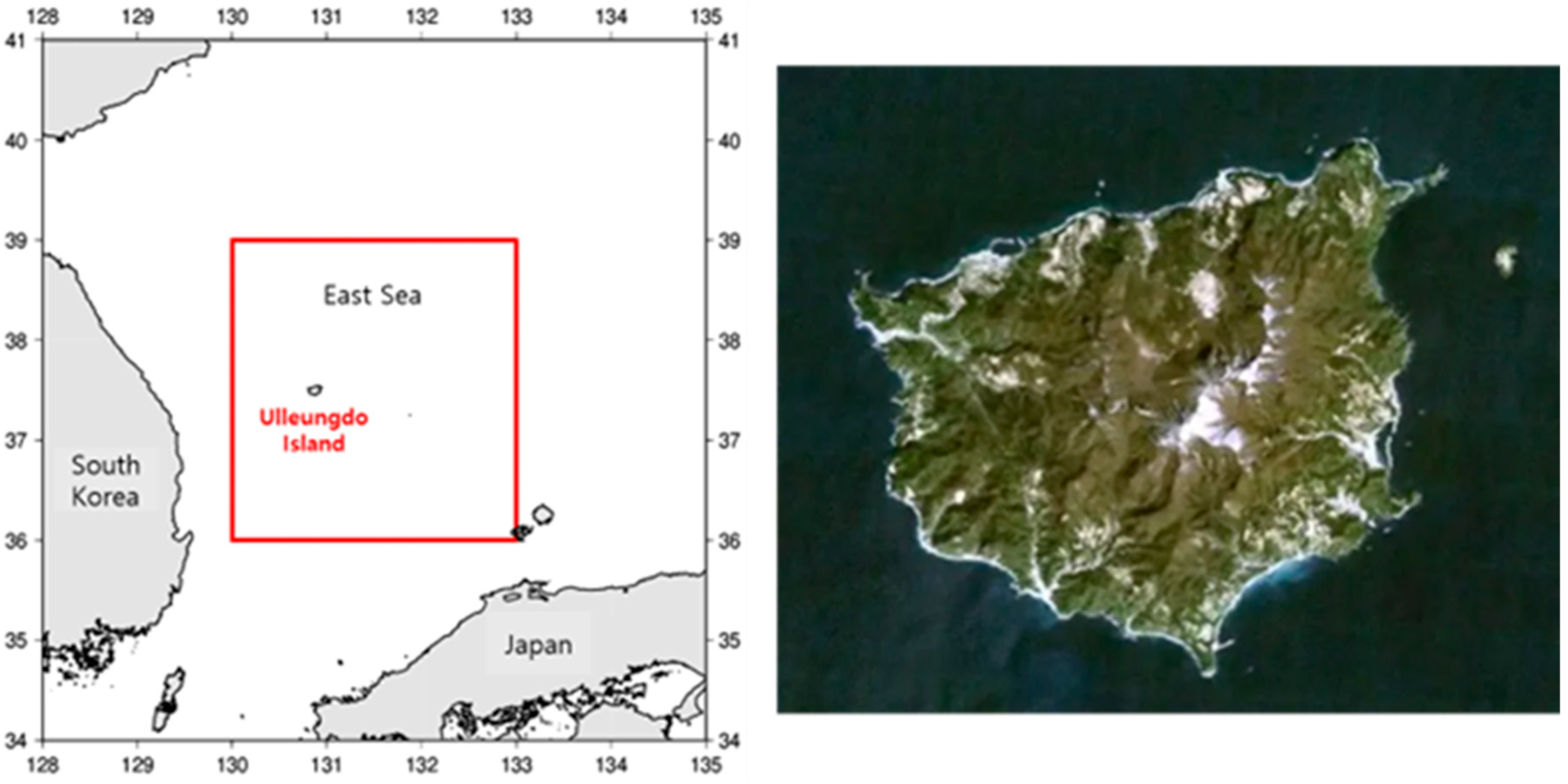
This study aims to estimate the long-term mean sea level (MSL) and update the elevation of the tidal datum for Ulleungdo—an island region where direct leveling is not feasible—by utilizing extended tide gauge observation records. Ulleungdo maintains an independent vertical reference system, with its official datum elevation established based on approximately one year of tidal observations collected between 1 June 1975 and 30 May 1976. However, this duration is substantially shorter than the internationally recommended 18.6-year tidal cycle required for reliable MSL estimation. Consequently, there is a clear need to reassess and revise the existing datum elevation using MSL values computed from long-term observations that satisfy the global standard.
Previous research has consistently demonstrated that MSL exhibits a gradual upward trend over time, largely driven by climate change and global ocean warming. Accurate prediction of such long-term changes is crucial for improving vertical datum frameworks, particularly in regions with limited geodetic access. In this context, precise MSL forecasting can inform the selection of appropriate reference periods for datum establishment and facilitate the incorporation of sea level trends into elevation benchmarks, thereby enhancing the long-term stability and relevance of vertical control networks.
Figure 2 shows Geographical location and satellite view of Ulleungdo Island in the East Sea (Sea of Korea). The left panel shows the regional context of Ulleungdo, situated approximately 120 km east of the Korean Peninsula within the East Sea. The red box highlights the study area used for sea level trend analysis. The right panel presents a high-resolution satellite image of Ulleungdo Island, which serves as the primary location for tide gauge observations and vertical datum assessment in this study.

2.2. Deep Learning Algorithm

Recurrent neural networks (RNNs) are widely used for time series modeling due to their ability to capture temporal dependencies. [13,14,15,16,17] Among them, Long Short-Term Memory (LSTM) and Gated Recurrent Unit (GRU) models are particularly effective for sea level prediction, as they are capable of learning both short- and long-term patterns in sequential data. LSTM is known for its strength in modeling longer-term dependencies, while GRU offers a simpler structure with faster training and competitive accuracy. [18,19,20,21] This study evaluates and compares the performance of both models in predicting long-term mean sea level trends based on tide gauge observations from Ulleungdo.

2.2.1. Long Short-Term Memory (LSTM) Networks for Sequential Data Prediction

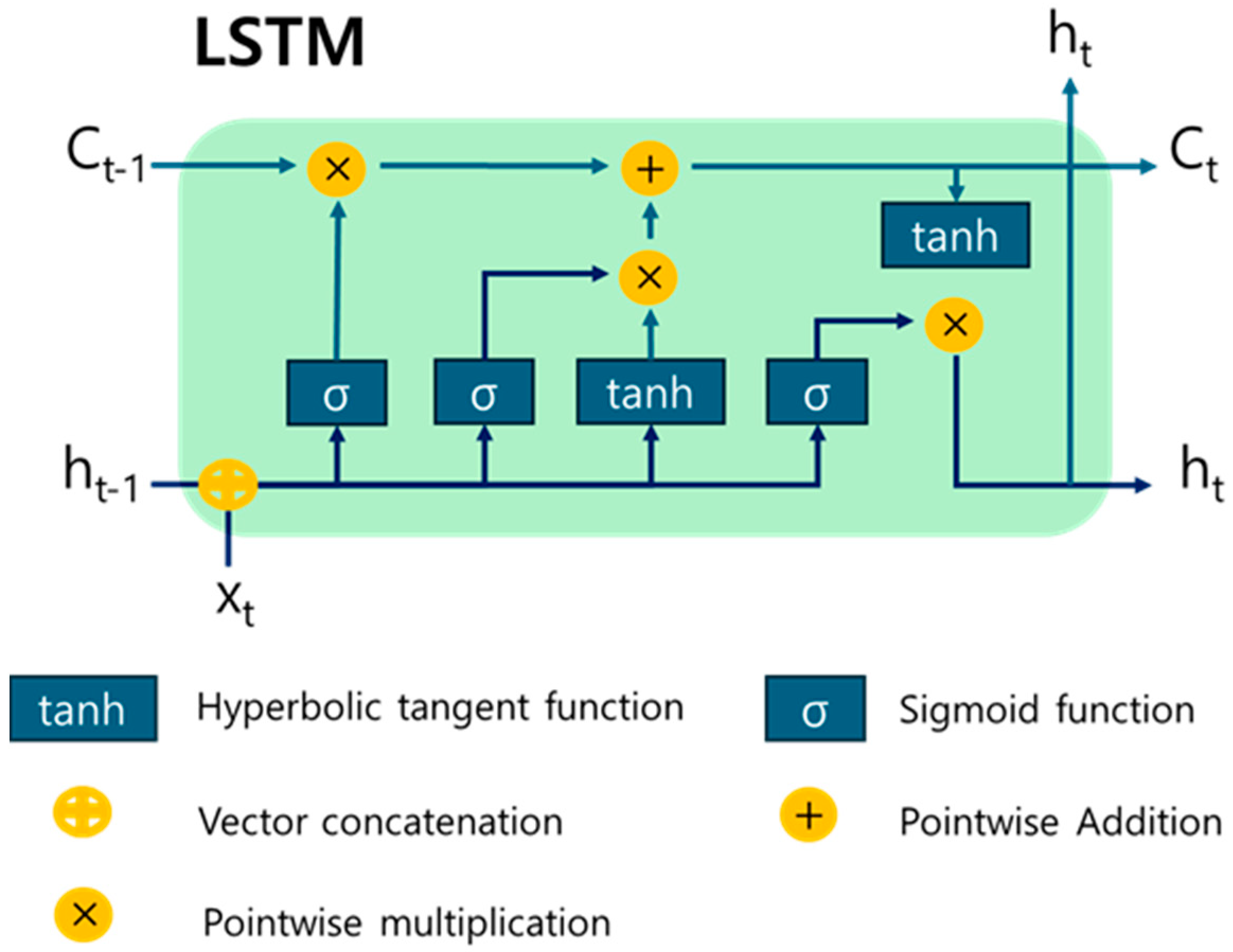
LSTM networks are an extension of traditional recurrent neural networks (RNNs) designed to overcome the vanishing gradient problem when learning from long sequences. The architecture introduces a memory cell and three gates—forget, input, and output—that control the selective retention, update, and release of information over time.
  • Forget gate: Decides which past information to retain.
  • Input gate: Determines which new information to incorporate.
  • Output gate: Controls how much information from the cell state is passed to the next layer or time step.
Using sigmoid and tanh activation functions, these gates enable the network to preserve long-term dependencies while discarding irrelevant data. Through this mechanism, LSTMs effectively capture both short- and long-term temporal patterns, making them well-suited for tasks such as time-series forecasting, speech recognition, and natural language processing, where sequential dependencies are critical.
Figure 3 shows schematic diagram of a Long Short-Term Memory (LSTM) unit showing the forget, input, and output gates. The sigmoid (σ) and tanh activations regulate how information is discarded, updated, and passed to the next time step, while addition (+) and multiplication (×) operations control the flow of data through the memory cell to capture both short- and long-term dependencies in sequential tasks.

2.2.2. Gated Recurrent Unit for Sequential Learning

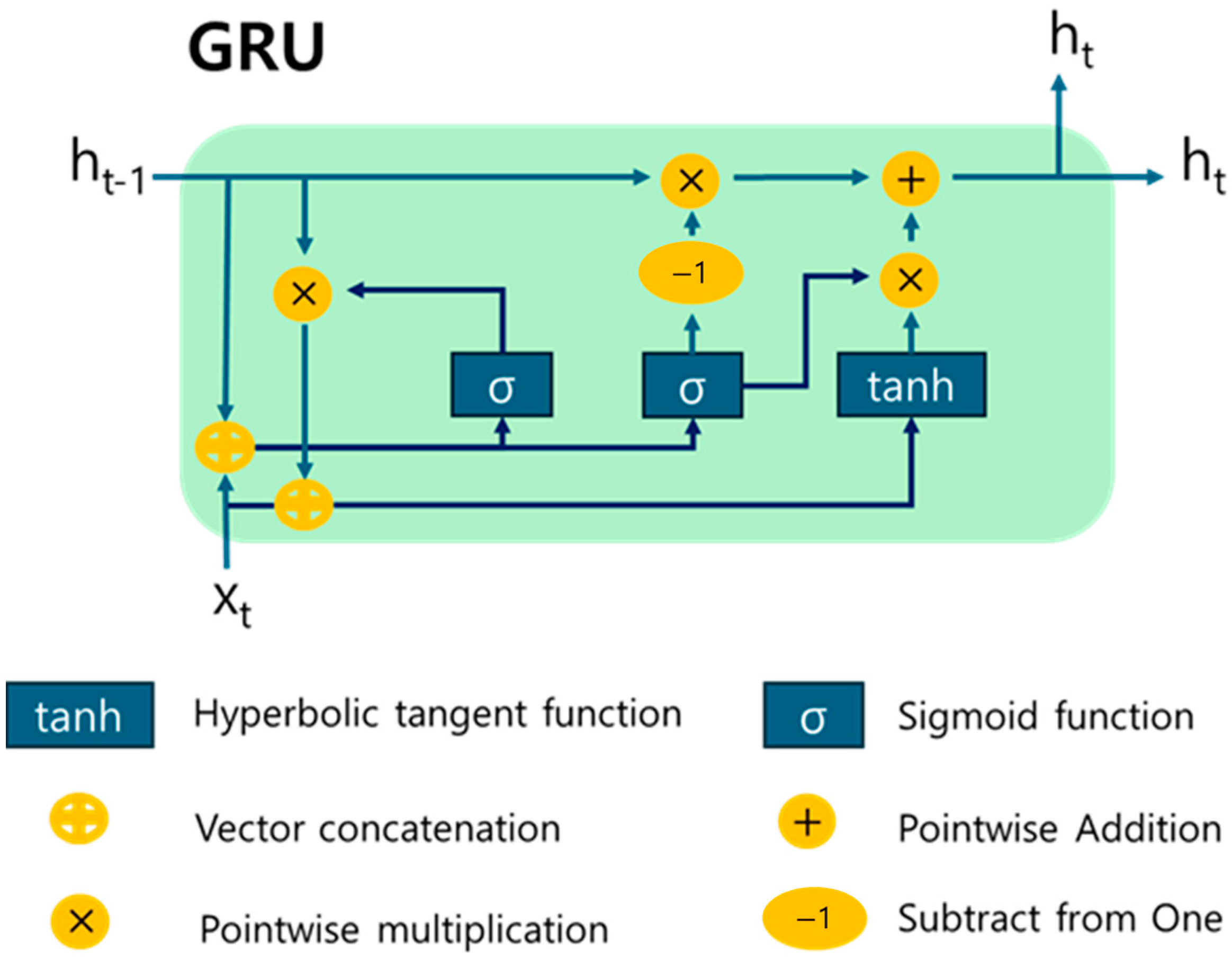
GRUs are a simplified variant of LSTMs that reduce model complexity while preserving the ability to capture both short- and long-term dependencies in sequential data. Unlike LSTMs, which use separate input and forget gates, GRUs combine them into a single update gate and introduce a reset gate to control how much past information is retained or discarded.
  • Update gate: balances new information and past memory to determine the final output.
  • Reset gate: controls how much previous information is ignored when processing new input.
Using sigmoid and tanh activations, GRUs efficiently manage information flow with fewer parameters than LSTMs, making them well-suited for time-series forecasting tasks, such as mean sea level prediction, where both computational efficiency and long-term memory are critical.
Figure 4 shows schematic diagram of the GRU model showing the reset and update gates. The reset gate discards irrelevant past information, while the update gate balances past memory and new data. Sigmoid (σ) and tanh activations control the flow of information, enabling efficient long-term dependency modeling with fewer parameters than LSTM.

2.2.3. Normalization and Data Structuring for Training

To promote numerical stability and enhance the convergence behavior of the deep learning model, it is essential to normalize all input variables within the dataset to a standardized scale prior to training. Normalization mitigates the risk of gradient instability caused by feature value disparities and ensures that each feature contributes proportionately to the learning process. Without such normalization, features with inherently large numerical ranges could disproportionately influence the loss function, leading to suboptimal or biased model performance. Furthermore, a consistent input range facilitates smoother optimization dynamics and accelerates convergence during gradient-based learning.
In this study, min–max normalization was employed to rescale all continuous variables to the range of [0, 1], a commonly adopted practice in deep learning applications. This transformation method preserves the relative relationships between data points while constraining all values within a bounded interval, which is particularly beneficial for activation functions sensitive to input magnitudes (e.g., sigmoid, ReLU). The normalization process was implemented as a preprocessing step applied uniformly across all relevant numerical features.
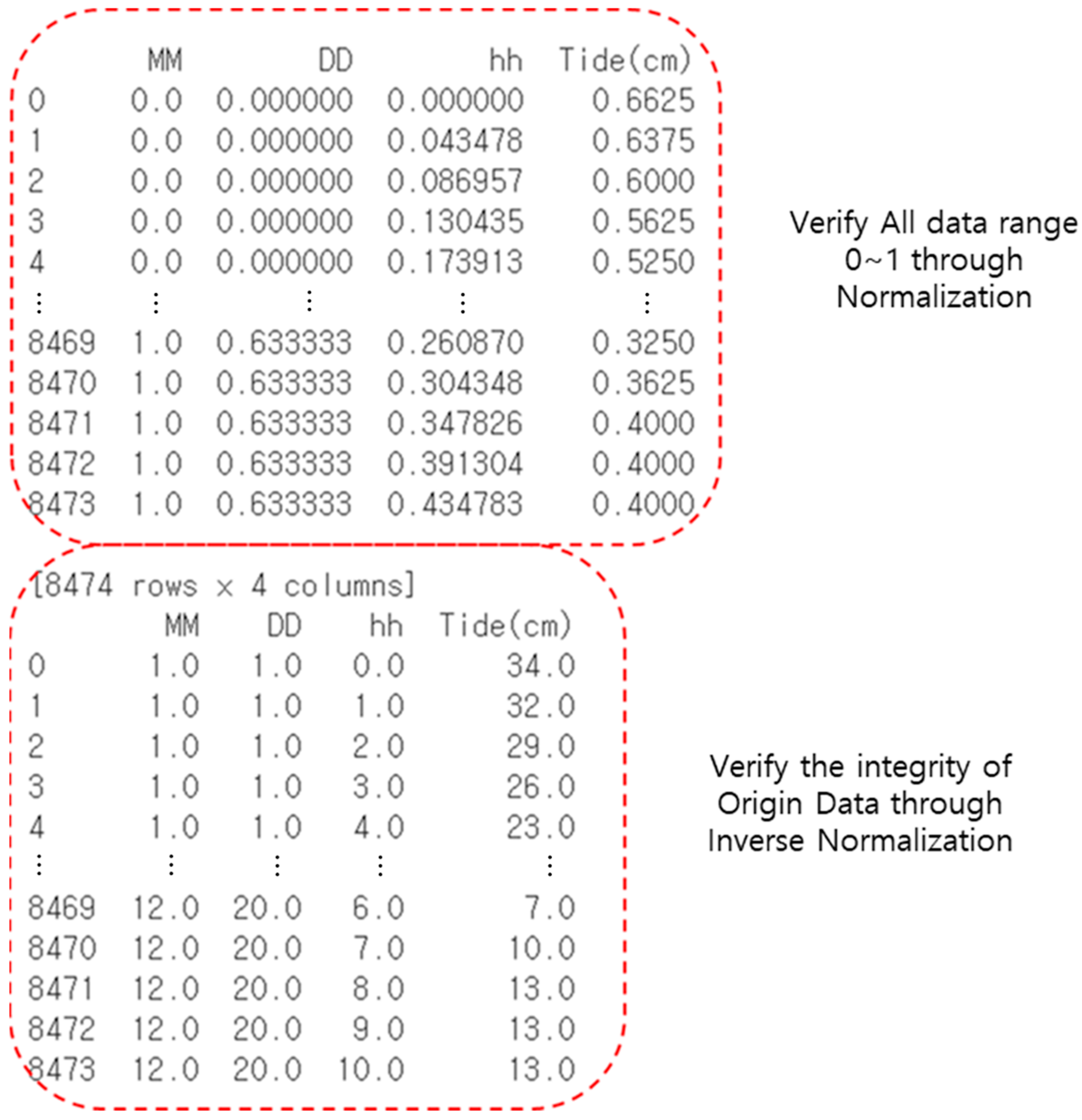
To ensure the accuracy and fidelity of the transformation, a two-step verification procedure was adopted. First, the raw dataset underwent min–max normalization using the recorded minimum and maximum values for each feature. Then, inverse normalization was performed to reconstruct the original data values from their normalized counterparts. This round-trip conversion allowed for quantitative and visual inspection of data integrity, ensuring that the normalization procedure did not introduce any rounding errors, numerical instability, or loss of precision.
The outcomes of this verification are presented in Figure 5. The upper panel illustrates the results of min–max normalization, where all data attributes were effectively scaled to the designated [0, 1] interval, thereby standardizing the feature space for subsequent model training. In contrast, the lower panel displays the results of inverse normalization, confirming that the original data structure and distribution were perfectly preserved through the bidirectional transformation process. No significant deviation, bias, or distortion was observed, validating the mathematical correctness and reversibility of the normalization scheme.
Following this validation, the normalized dataset was programmatically converted into NumPy array format to support seamless integration with the deep learning framework adopted in this study. The use of NumPy arrays enabled vectorized computation, efficient memory management, and high-throughput data handling during training. This array-based representation also allowed for streamlined preprocessing, augmentation, and batching procedures, thereby optimizing the data input pipeline and ensuring compatibility with GPU-accelerated model execution environments.
In summary, the combination of normalization, inverse validation, and array transformation constituted a robust and reproducible data preprocessing pipeline. This ensured numerical stability, preserved data integrity, and facilitated efficient training, all of which are critical prerequisites for the successful deployment of deep learning models in high-resolution geospatial or sensor-based applications.

2.2.4. Prediction Model Set Up

In this study, the predictive performance of the LSTM and GRU models was evaluated using hourly tide observations collected from 2000 to 2018. Each annual dataset contained approximately 8760 data points, and the entire dataset comprised 192,720 hourly observations (19 years × 8760 h). The data were divided into training, validation, and test subsets with a ratio of 90%:5%:5%.
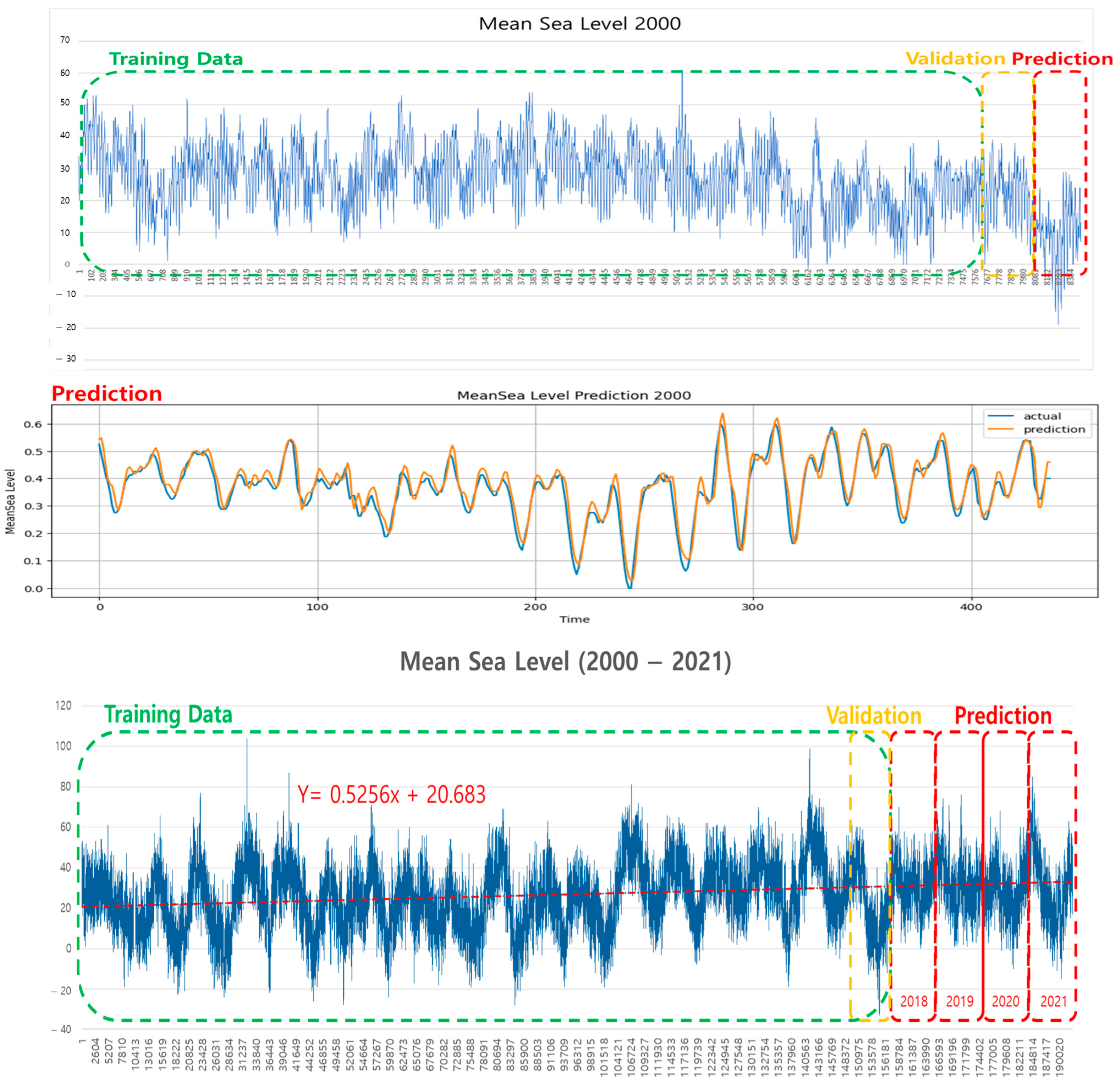
The models were designed to use N days of past data as input to generate N/24 outputs, a process repeated 24 times to obtain one full day of predictions (24 hourly values). This design reflects the daily periodic pattern of tides and diurnal cycles. On average, about 435 tide values were predicted per year, corresponding to approximately 18–19 days.
The predictive performance of the two models was compared over the 2000–2018 period, and the model with relatively higher accuracy was then applied to forecast annual mean sea level for 2018, 2019, 2020, and 2021 using the same approach.
Figure 6 shows Machine learning model performance for mean sea level prediction (2000–2021). (Top panel) Time series of mean sea level in 2000 showing training data (green dashed box), validation period (yellow dashed box), and prediction period (red dashed box). (Middle panel) Comparison between actual observations (blue line) and model predictions (orange line) for mean sea level in 2000, demonstrating close agreement between predicted and observed values. (Bottom panel) Complete mean sea level time series from 2000 to 2021 with linear trend line (Y = 0.5256 x + 20.683, red line) overlaid on the data. The dataset is partitioned into training (green dashed box), validation (yellow dashed box), and multi-year prediction periods (2018–2021, red dashed boxes), illustrating the model’s capacity to capture both short-term variability and long-term trends in sea level dynamics.

2.3. Model Performance Test

Regression models are typically evaluated using various metrics that provide different insights into model accuracy and error characteristics. Common metrics include Mean Absolute Error (MAE), Mean Squared Error (MSE), Mean Absolute Percentage Error (MAPE), and Root Mean Squared Error (RMSE).
The Mean Absolute Error (MAE) calculates the average of the absolute differences between the actual values (yᵢ) and the predicted values ( y i ^ ). This metric is less sensitive to outliers, making it particularly useful when robustness is required. It is defined by the following formula [22]:
MAE = 1 n i = 1 n y i y l ^
where
  • y i represents the actual value;
  • y l ^ represents the predicted value;
  • n is the number of data points.
This formula reflects the average of the absolute errors between the predicted and actual values, with each error given equal weight.
The Mean Squared Error (MSE), on the other hand, computes the average of the squared differences between actual and predicted values. The squaring process amplifies larger errors, making MSE more sensitive to outliers. This is particularly useful when large deviations are undesirable. The formula for MSE is Dumre et al., [22]:
M S E = 1 n i = 1 n y i y l ^ 2
The Root Mean Squared Error (RMSE) is the square root of the MSE. RMSE is interpretable in the same units as the original values, which makes it more intuitive. This metric also emphasizes larger errors and is useful when errors are expected to be normally distributed. The RMSE formula is Chai and Draxler [22,23]:
R M S E = 1 n i = 1 n y i y l ^ 2
Finally, the Mean Absolute Percentage Error (MAPE) calculates the average of the absolute percentage differences between the actual and predicted values, making it scale-independent. However, MAPE can be problematic when actual values are close to zero, as it can lead to large, unstable percentage errors. The formula for MAPE is (Airlangga, Jain et al., [24,25]:
M A P E = 100 n i = 1 n y i y l ^ y i
where
  • y i represents the actual value,
  • y l ^ represents the predicted value,
  • n is the number of data points, and
The expression |( y i y l ^ )/ y i | represents the absolute percentage error.
Among the various deep learning algorithms, algorithms such as CNN have demonstrated high performance in computer vision domains such as image classification and optical flow. Meanwhile, RNN tends to be useful for predicting future sequences based on past learning. In RNNs, the current output is influenced by the results of the previous time step, and the hidden layer acts as a kind of memory. This structure is expected to be particularly suitable for predicting mean sea level, which exhibits strong periodicity. In this study, we apply and compare the performance of RNN-based LSTM and GRU models to propose the most appropriate model for prediction.
LSTM consists of a structure in which multiple gates exist within a single cell, and these gates form a chain-like architecture. These gates are responsible for controlling, protecting, forgetting, inputting, and outputting the cell’s contents, which are then passed on to the next cell. The input and output gates define the data used as input and output, respectively. The forget gate decides whether to retain or discard previous information, while the next input gate uses weights to determine what portion of the newly incoming information to store or discard, ultimately creating the new state of the cell. This process is repeated to form a logical structure for predicting the next value.
Compared to traditional neural networks, the LSTM network includes additional components such as cells, input gates, output gates, and forget gates. The cell is a component that preserves memory according to the unit time of the given input data. The input gate is a neural network layer that regulates data flow into the cell. The output gate functions similarly but regulates the flow of data out of the cell. The forget gate is used to erase unnecessary memories.
In this method, the input gate incorporates periodic and consistent movements such as the gravitational motion of the sun and moon, the annual movement of tectonic plates, and seasonal changes in wind speed and direction. The output gate is set to the long-term sea level change over 21 years used in this study, thereby enabling an integrated prediction of various factors influencing the mean sea level. Theoretically, the relative positions of the sun and moon can be reflected on an hourly basis, and factors such as wind speed and direction, mean sea-level pressure, and near-surface air temperature can be incorporated to account for seasonality in sea level, allowing for more accurate predictions of future mean sea level variations.
The models were trained using hourly tide level data recorded at tide gauge stations, comprising approximately 8760 values per year from 2000 to 2018. The dataset was divided into Training (7884) and Validation/Prediction (438), and model performance was evaluated using RMSE and R2.
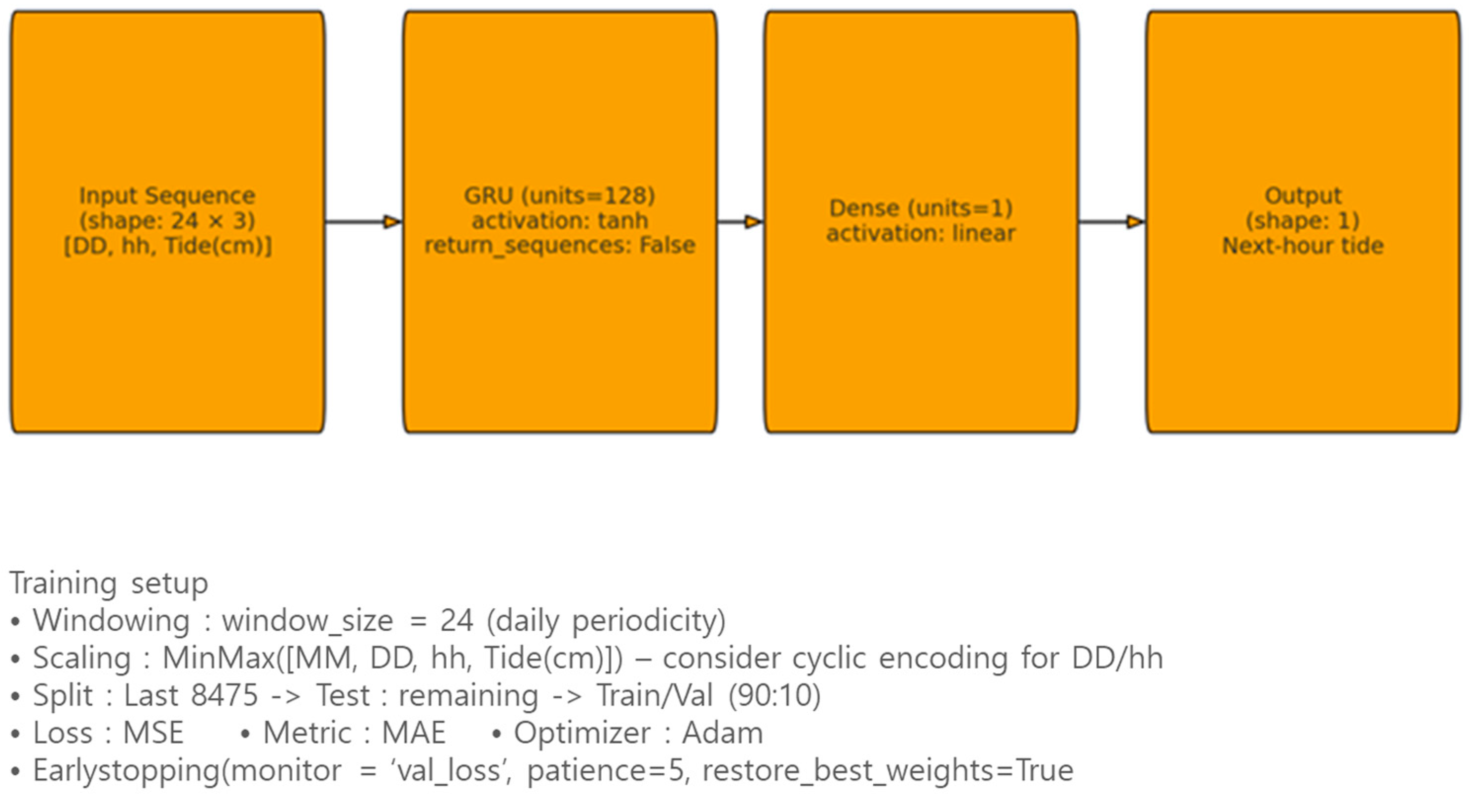
Figure 7 Shows network architecture of the GRU-based sea level prediction model. The model receives an input sequence of 24 consecutive hourly records consisting of day, hour, and tide height values. A single GRU layer with 128 units and tanh activation captures the temporal dependencies, followed by a dense layer with linear activation to output the predicted tide level for the next hour. The training setup incorporates Min–Max normalization, a data split into training, validation, and test sets, and early stopping to prevent overfitting.

3. Results

3.1. Data Preprocessing

The initial and critical phase in preparing the dataset for deep learning model training involves comprehensive data preprocessing. This step ensures the reliability and integrity of the input data by addressing anomalies such as outliers and missing values. Outliers—defined as observations that deviate significantly from the expected statistical distribution—were identified and either excluded or replaced with contextually appropriate values to minimize their influence on the model’s learning process.
A common challenge associated with mean sea level datasets is the presence of missing values, which can degrade model performance if left unaddressed. Similarly to outliers, these gaps must be systematically identified and handled. In this study, widely adopted functions from the Python(ver 3.12.12) pandas library, including isnull() and sum(), were employed to detect and quantify the extent of missing data. Rows or columns containing missing or anomalous entries were then either removed or imputed based on predefined criteria.
Through this preprocessing procedure, the dataset was thoroughly cleansed by examining all relevant attributes, ensuring the removal of inconsistencies and incomplete records. The result was a robust and high-quality dataset suitable for subsequent deep learning model training and evaluation. Table 1 summarizes the key hyperparameters and model settings used in the deep learning architecture for training and evaluation.

3.2. Performance Evaluation and Prediction Using the GRU Model

To evaluate the model’s predictive capabilities, a comparative analysis between LSTM and GRU architectures was conducted using the Root Mean Square Error (RMSE) as the primary performance metric. Based on the results, the GRU model demonstrated slightly superior accuracy and was thus selected for predicting annual mean sea level. This section presents the detailed performance evaluation of both models and describes the application of the GRU model for future sea level prediction from 2018 to 2021.
Table 2 presents the annual RMSE values obtained from the LSTM and GRU models for the period 2000–2018, along with the overall average, enabling a comparative assessment of each model’s prediction accuracy.
This performance advantage of the GRU model can be attributed to its simplified architecture, where the input and forget gates of the LSTM are combined into a single update gate. This reduction in parameters allows the GRU to capture temporal dependencies more efficiently while mitigating overfitting risks, leading to faster training and slightly better generalization on the available dataset.
Nevertheless, the results also suggest that the standard LSTM model itself is capable of delivering meaningful and robust predictive performance, indicating that both architectures remain valuable for time-series forecasting tasks.
As shown in Table 2, both the LSTM and GRU models exhibited consistently low RMSE values across the 19-year evaluation period, indicating robust predictive performance. However, the GRU model outperformed the LSTM model in the majority of years, yielding a lower average RMSE of 0.0215793 compared to 0.0243295 for the LSTM model. This performance margin, though modest, reflects the GRU model’s relative efficiency in capturing temporal dependencies in the normalized annual sea level data. Based on these findings, the GRU architecture was selected as the preferred model for future sea level forecasting due to its superior accuracy, reduced computational complexity, and faster convergence characteristics.

3.3. Statistical Analysis of Predicted Values

Following the comparative evaluation presented in the previous section, the GRU model—demonstrating slightly superior prediction accuracy—was selected for forecasting annual mean sea levels. The model development pipeline, including data preprocessing, normalization, training data generation, and evaluation procedures, remained consistent with the approach previously applied to the LSTM model to ensure methodological comparability. Using this optimized GRU-based framework, sea level predictions were generated for the years 2018 through 2021. The year 2018 was of particular interest as it represents the culmination of an 18.6-year tidal cycle, while the subsequent years fall within the early phase of the next cycle. Although 2022 predictions were also computed, incomplete observational data for that year precluded its inclusion in graphical comparisons with observed values. Apart from adjustments to the input data window, all model parameters were retained to ensure consistency in evaluation.
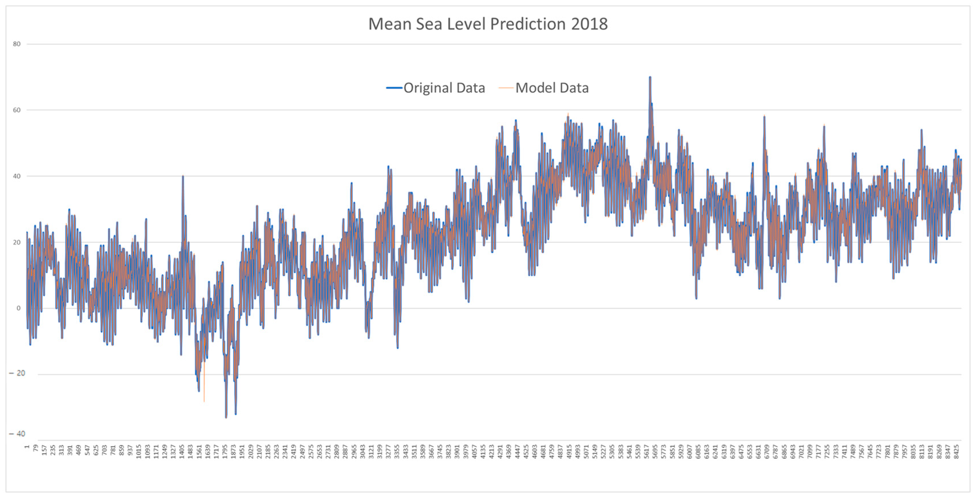
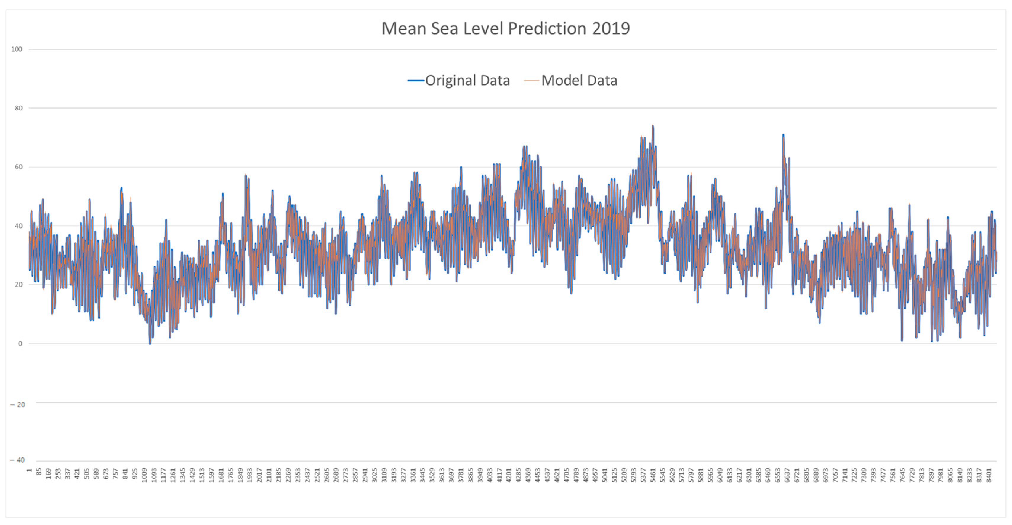
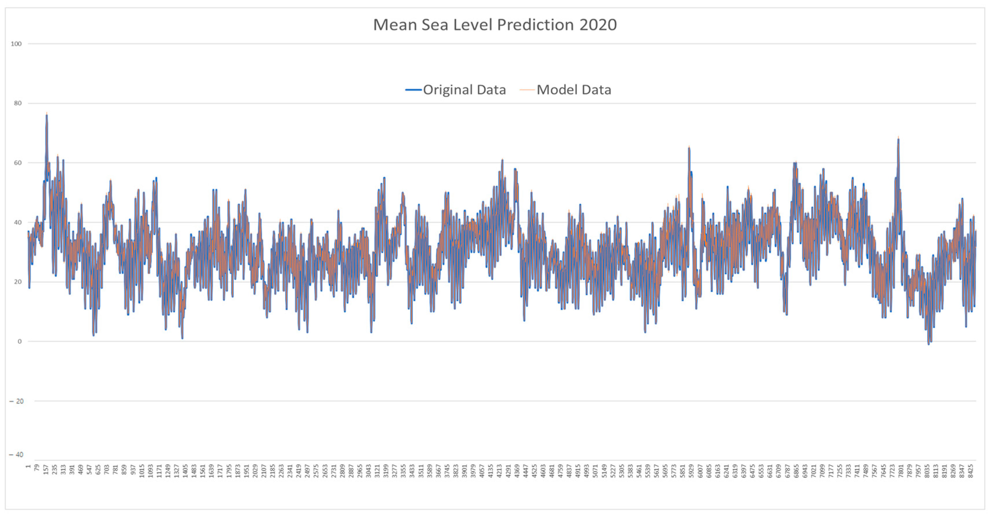
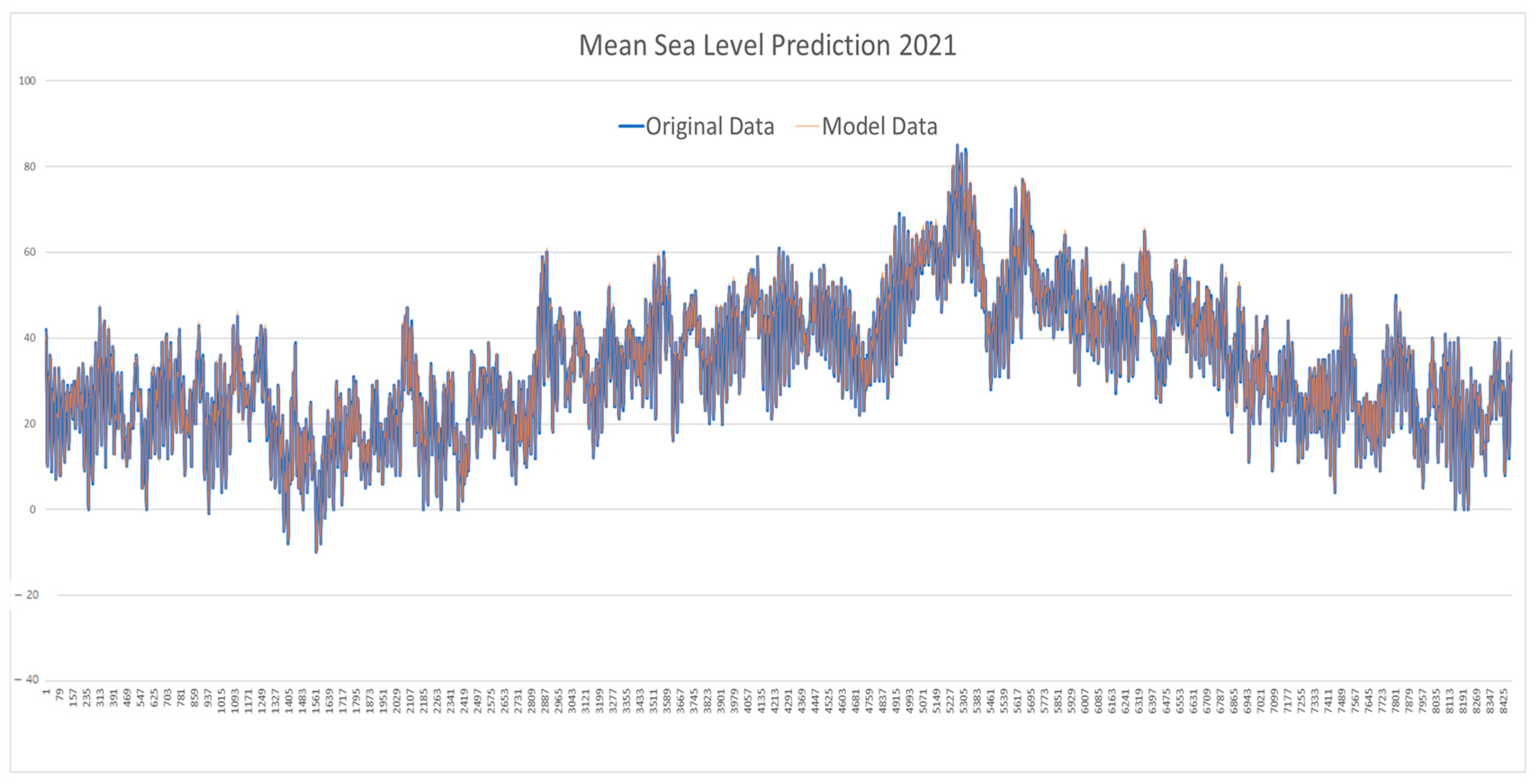
Table 3 presents the statistical summary of the GRU model’s annual mean sea level predictions from 2018 to 2021, including minimum, maximum, mean, standard deviation (SD), and root mean square error (RMSE) values. A graphical comparison between the predicted and observed values for this period is provided in Appendix A.

4. Discussion

This study presents a deep learning-based framework for predicting annual mean sea level (MSL) using GRU and LSTM architectures, with a focus on the Ulleungdo region—a geodetically isolated area with a legacy vertical datum based on limited observation periods. The research demonstrates that the proposed GRU model offers slightly superior performance compared to the LSTM model in terms of RMSE, achieving an average error of 0.0216 compared to 0.0243 across an 18-year span. The low prediction errors and stable trend patterns confirm the feasibility of using GRU for long-term MSL estimation in coastal and island regions.

4.1. Strengths of the Study

One of the primary strengths lies in the methodical construction and evaluation of the GRU model using long-term observational data that captures an entire 18.6-year tidal epoch. The study rigorously applies normalization, inverse normalization validation, and thorough statistical analyses to ensure model fidelity and reproducibility. The comparative evaluation of GRU and LSTM under identical preprocessing conditions strengthens the reliability of the conclusions drawn. Moreover, the study provides insights into the potential use of deep learning for geodetic applications such as vertical datum updating, especially in regions where traditional leveling is impractical.
Another strength is the careful treatment of data quality during preprocessing. By addressing missing values and outliers and verifying normalization integrity, the authors ensure that the input to the deep learning models reflects true oceanographic trends rather than data noise or artifacts. The use of RMSE-based yearly evaluations enhances transparency and allows for granular performance assessment across time.
In addition, the proposed framework offers a clear advantage over traditional approaches for mean sea level determination, such as harmonic analysis and Doodson’s filtering. While these conventional methods are well established, they require the estimation of numerous harmonic constants, making the process mathematically complex and computationally demanding. By contrast, the deep learning approach presented here is able to achieve high predictive accuracy once long-term observational records are available, without the explicit calculation of harmonic parameters. This data-driven flexibility highlights the potential of deep learning methods to complement or even substitute conventional techniques, particularly in regions where extended tidal records are reliably secured.

4.2. Limitations and Areas for Improvement

Despite the predictive performance demonstrated, several limitations must be acknowledged. First, the model relies solely on sea level time series data without incorporating auxiliary predictors such as atmospheric pressure, sea surface temperature, wind variability, greenhouse gas forcing, or ocean current changes. These climate-driven variables significantly influence regional sea level variability, and their exclusion may constrain the model’s generalizability to more dynamic coastal settings.
Second, while the study successfully applies GRU to a localized site, it does not extend the framework to other tide stations for comparative validation. Given the variability in coastal hydrodynamics and sensor environments, the robustness of the model across spatially diverse regions remains uncertain. Additionally, although the GRU model performed slightly better, the performance difference was marginal. More advanced architectures such as attention-based models (e.g., Transformer, Temporal Fusion Transformer) or hybrid frameworks could further improve performance, especially for long-term forecasting.
Lastly, the absence of uncertainty quantification (e.g., confidence intervals or prediction intervals) limits the interpretability of the results, particularly in the context of risk-informed coastal planning or infrastructure design.

4.3. Future Research Directions

To enhance the utility, robustness, and generalizability of the proposed deep learning framework for mean sea level (MSL) prediction, several promising research directions are identified based on recent literature.
First, incorporating exogenous climate variables—such as ENSO indices, barometric pressure, and sea surface temperature (SST)—within a multivariate modeling framework can improve the model’s ability to capture complex, non-stationary climate signals. According to Ham et al. [26], Zhou and Zhang [27], and Mu et al. [28], the inclusion of such variables, particularly when used in conjunction with advanced neural architectures like CNNs and Transformers, has been shown to significantly improve the predictability of large-scale phenomena such as ENSO and SST anomalies.
Second, expanding spatial coverage by applying the model to multiple tide gauge stations across the Korean Peninsula and East Asia can support the development of ensemble or federated learning approaches. As suggested by Vadivel et al. [29], such strategies can improve spatial generalization by aggregating predictions across locations while accounting for local heterogeneity and sensor biases. This is especially important in regions where tide gauge records are affected by differential land motion and localized oceanographic conditions. However, securing more than 18.6 years of continuous observations from tide gauge stations across the Republic of Korea has been challenging. Future work will prioritize collecting sufficiently long-term datasets from multiple stations sharing the same coastal boundaries to enable comprehensive spatial modeling.
Third, the integration of uncertainty quantification methods—such as Monte Carlo dropout, Bayesian neural networks, and quantile regression—can enhance the interpretability and credibility of sea level forecasts. According to Wang et al. [30] and Sun et al. [31], incorporating these techniques allows models to better communicate confidence intervals and identify prediction uncertainty, which is crucial for decision-making in coastal hazard mitigation and infrastructure adaptation planning.
Finally, from a geodetic perspective, future work should explore the fusion of predicted sea level trends with GNSS-derived vertical land motion (VLM) data. Studies by Vadivel et al. [32,33] have shown that integrating InSAR or GNSS data with tide gauge observations enables more accurate estimation of absolute sea level change by compensating for local subsidence or uplift. Such integration would also support the establishment of a dynamic vertical datum system that evolves with ongoing sea level rise and land deformation processes.

5. Conclusions

This study developed and validated a deep learning-based prediction framework for annual mean sea level estimation, focusing on the Ulleungdo region in the East Sea. Using long-term tidal observation data spanning the full 18.6-year nodal cycle, two recurrent neural network architectures—LSTM and GRU—were evaluated in terms of their predictive accuracy. Both models demonstrated strong performance; however, the GRU model yielded slightly lower RMSE values and more stable trend representations, leading to its selection for final prediction modeling.
The GRU-based model effectively reproduced sea level patterns and demonstrated excellent agreement with observed data from 2018 to 2021, confirming its potential for practical application in sea level forecasting. This framework holds particular relevance for regions like Ulleungdo, where conventional leveling techniques for vertical datum management are limited. By leveraging time series learning, the proposed model offers a data-driven alternative for supporting geodetic datum updates and monitoring regional sea level changes.
While satisfactory predictive performance was achieved using LSTM and GRU, future work will extend this framework to more structurally complex neural architectures, such as CNN-LSTM hybrids or Transformer-based models, which may further improve long-term forecasting capability. Despite its strengths, the present model’s performance could also be enhanced through the integration of exogenous environmental variables (e.g., atmospheric pressure, sea surface temperature, wind variability, ocean current changes, and greenhouse gas forcing) and broader spatial validation across additional tide stations. Incorporating uncertainty quantification and vertical land motion data would further enable absolute sea level change estimation.
In summary, the proposed deep learning approach provides a reliable and scalable solution for long-term sea level prediction in coastal and island environments. It contributes to the advancement of geodetic applications and supports data-informed decision-making for infrastructure resilience, coastal planning, and climate adaptation strategies.

Author Contributions

Conceptualization, T.-Y.K., S.-J.L., H.-S.Y. and H.-M.Y.; methodology, T.-Y.K., S.-J.L. and H.-M.Y.; software, T.-Y.K., S.-J.L. and H.-M.Y.; validation, T.-Y.K., S.-J.L. and H.-S.Y.; formal analysis, T.-Y.K., S.-J.L. and H.-M.Y.; investigation, T.-Y.K., S.-J.L. and H.-M.Y.; resources, T.-Y.K., S.-J.L. and H.-M.Y.; data curation, T.-Y.K., S.-J.L. and H.-M.Y.; writing—original draft preparation, T.-Y.K., S.-J.L. and H.-M.Y.; writing—review and editing, H.-S.Y. and H.-M.Y.; visualization, T.-Y.K. and S.-J.L.; supervision, H.-S.Y.; project administration, H.-S.Y.; funding acquisition, H.-S.Y. All authors have read and agreed to the published version of the manuscript.

Funding

This research was supported by the BK21 FOUR Program (Graduate School Innovation) funded by the Ministry of Education (MOE, Republic of Korea) and the National Research Foundation of Korea (NRF). No specific grant number is assigned to this program.

Institutional Review Board Statement

Not applicable.

Informed Consent Statement

Not applicable.

Data Availability Statement

The original contributions presented in the study are included in the article; further inquiries can be directed to the corresponding authors.

Conflicts of Interest

The authors declare no conflicts of interest.

Appendix A

Graphical comparisons between the GRU model’s predicted annual mean sea levels and the corresponding observed values for the years 2018 to 2021 are presented below.
Figure A1. Comparison between the GRU model’s predicted sea level data (Model Data) and observed sea level measurements (Original Data) for the year 2018. The figure illustrates the high temporal alignment between the two time series over the full year, reflecting the model’s capability to capture both the trend and short-term variability in annual mean sea level. Notably, the prediction aligns closely with observed fluctuations, particularly during periods of tidal amplitude variation, thereby validating the model’s reliability for practical forecasting applications.
Applsci 15 11067 g0a1
Figure A2. Comparison between the GRU model’s predicted sea level data (Model Data) and observed sea level measurements (Original Data) for the year 2019. The figure illustrates the high temporal alignment between the two time series over the full year, reflecting the model’s capability to capture both the trend and short-term variability in annual mean sea level. Notably, the prediction aligns closely with observed fluctuations, particularly during periods of tidal amplitude variation, thereby validating the model’s reliability for practical forecasting applications.
Applsci 15 11067 g0a2
Figure A3. Comparison between the GRU model’s predicted sea level data (Model Data) and observed sea level measurements (Original Data) for the year 2020. The figure illustrates the high temporal alignment between the two time series over the full year, reflecting the model’s capability to capture both the trend and short-term variability in annual mean sea level. Notably, the prediction aligns closely with observed fluctuations, particularly during periods of tidal amplitude variation, thereby validating the model’s reliability for practical forecasting applications.
Applsci 15 11067 g0a3
Figure A4. Comparison between the GRU model’s predicted sea level data (Model Data) and observed sea level measurements (Original Data) for the year 2021. The figure illustrates the high temporal alignment between the two time series over the full year, reflecting the model’s capability to capture both the trend and short-term variability in annual mean sea level. Notably, the prediction aligns closely with observed fluctuations, particularly during periods of tidal amplitude variation, thereby validating the model’s reliability for practical forecasting applications.
Applsci 15 11067 g0a4

References

  1. Raj, N.; Brown, J. Prediction of Mean Sea Level with GNSS-VLM Correction Using a Hybrid Deep Learning Model in Australia. Remote Sens. 2023, 15, 2881. [Google Scholar] [CrossRef]
  2. Raj, N. Prediction of Sea Level with Vertical Land Movement Correction Using Deep Learning. Mathematics 2022, 10, 4533. [Google Scholar] [CrossRef]
  3. Rus, M.; Mihanović, H.; Ličer, M.; Kristan, M. HIDRA3: A Deep-Learning Model for Multipoint Ensemble Sea Level Forecasting in the Presence of Tide Gauge Sensor Failures. Geosci. Model Dev. 2025, 18, 605–620. [Google Scholar] [CrossRef]
  4. Hassan, K.M.d.A. Predicting Future Global Sea Level Rise From Climate Change Variables Using Deep Learning. Int. J. Comput. Digit. Syst. 2023, 13, 829–836. [Google Scholar] [CrossRef]
  5. Liu, J.; Jin, B.; Wang, L.; Xu, L. Sea Surface Height Prediction With Deep Learning Based on Attention Mechanism. IEEE Geosci. Remote Sens. Lett. 2022, 19, 1–5. [Google Scholar] [CrossRef]
  6. Song, T.; Han, N.; Zhu, Y.; Li, Z.; Li, Y.; Li, S.; Peng, S. Application of Deep Learning Technique to the Sea Surface Height Prediction in the South China Sea. Acta Oceanol. Sin. 2021, 40, 68–76. [Google Scholar] [CrossRef]
  7. Bahari, N.A.A.B.S.; Ahmed, A.N.; Chong, K.L.; Lai, V.; Huang, Y.F.; Koo, C.H.; Ng, J.L.; El-Shafie, A. Predicting Sea Level Rise Using Artificial Intelligence: A Review. Arch. Comput. Methods Eng. 2023, 30, 4045–4062. [Google Scholar] [CrossRef]
  8. Hassanpour, H.; Corbett, B.; Mhaskar, P. Artificial Neural Network-Based Model Predictive Control Using Correlated Data. Ind. Eng. Chem. Res. 2022, 61, 3075–3090. [Google Scholar] [CrossRef]
  9. Bao, Y.; Mohammadpour Velni, J. A Hybrid Neural Network Approach for Adaptive Scenario-Based Model Predictive Control in the LPV Framework. IEEE Control Syst. Lett. 2023, 7, 1921–1926. [Google Scholar] [CrossRef]
  10. Abaza, B.F.; Gheorghita, V. Artificial Neural Network Framework for Hybrid Control and Monitoring in Turning Operations. Appl. Sci. 2025, 15, 3499. [Google Scholar] [CrossRef]
  11. Choi, Y.J.; Park, B.R.; Hyun, J.Y.; Moon, J.W. Development of an Adaptive Artificial Neural Network Model and Optimal Control Algorithm for a Data Center Cyber–Physical System. Build. Environ. 2022, 210, 108704. [Google Scholar] [CrossRef]
  12. Wang, D.; Shen, Z.J.; Yin, X.; Tang, S.; Liu, X.; Zhang, C.; Wang, J.; Rodriguez, J.; Norambuena, M. Model Predictive Control Using Artificial Neural Network for Power Converters. IEEE Trans. Ind. Electron. 2022, 69, 3689–3699. [Google Scholar] [CrossRef]
  13. Lipton, Z.C.; Berkowitz, J.; Elkan, C. A Critical Review of Recurrent Neural Networks for Sequence Learning. arXiv 2015, arXiv:1506.00019. [Google Scholar] [CrossRef]
  14. Kanagachidambaresan, G.R.; Ruwali, A.; Banerjee, D.; Prakash, K.B. Recurrent Neural Network. In Programming with TensorFlow; Prakash, K.B., Kanagachidambaresan, G.R., Eds.; EAI/Springer Innovations in Communication and Computing; Springer International Publishing: Cham, Switzerland, 2021; pp. 53–61. ISBN 978-3-030-57076-7. [Google Scholar]
  15. White, L.; Togneri, R.; Liu, W.; Bennamoun, M. Recurrent Neural Networks for Sequential Processing. In Neural Representations of Natural Language; Studies in Computational Intelligence; Springer: Singapore, 2019; Volume 783, pp. 23–36. ISBN 978-981-13-0061-5. [Google Scholar]
  16. Donkers, T.; Loepp, B.; Ziegler, J. Sequential User-Based Recurrent Neural Network Recommendations. In Proceedings of the Proceedings of the Eleventh ACM Conference on Recommender Systems, Como, Italy, 27 August 2017; ACM: New York, NY, USA, 2017; pp. 152–160. [Google Scholar]
  17. Yu, Y.; Si, X.; Hu, C.; Zhang, J. A Review of Recurrent Neural Networks: LSTM Cells and Network Architectures. Neural Comput. 2019, 31, 1235–1270. [Google Scholar] [CrossRef]
  18. Van Houdt, G.; Mosquera, C.; Nápoles, G. A Review on the Long Short-Term Memory Model. Artif. Intell. Rev. 2020, 53, 5929–5955. [Google Scholar] [CrossRef]
  19. Lindemann, B.; Müller, T.; Vietz, H.; Jazdi, N.; Weyrich, M. A Survey on Long Short-Term Memory Networks for Time Series Prediction. Procedia CIRP 2021, 99, 650–655. [Google Scholar] [CrossRef]
  20. Hochreiter, S.; Schmidhuber, J. Long Short-Term Memory. Neural Comput. 1997, 9, 1735–1780. [Google Scholar] [CrossRef]
  21. Dumre, P.; Bhattarai, S.; Shashikala, H.K. Optimizing Linear Regression Models: A Comparative Study of Error Metrics. In Proceedings of the 2024 4th International Conference on Technological Advancements in Computational Sciences (ICTACS), Tashkent, Uzbekistan, 13 November 2024; IEEE: Piscataway, NJ, USA, 2024; pp. 1856–1861. [Google Scholar]
  22. Chai, T.; Draxler, R.R. Root Mean Square Error (RMSE) or Mean Absolute Error (MAE)?—Arguments against Avoiding RMSE in the Literature. Geosci. Model Dev. 2014, 7, 1247–1250. [Google Scholar] [CrossRef]
  23. Hodson, T.O. Root-Mean-Square Error (RMSE) or Mean Absolute Error (MAE): When to Use Them or Not. Geosci. Model Dev. 2022, 15, 5481–5487. [Google Scholar] [CrossRef]
  24. Airlangga, G. A Comparative Analysis of Machine Learning Models for Predicting Student Performance: Evaluating the Impact of Stacking and Traditional Methods. Brilliance 2024, 4, 491–499. [Google Scholar] [CrossRef]
  25. Jain, P.; Sahoo, P.K.; Khaleel, A.D.; Al-Gburi, A.J.A. Enhanced Prediction of Metamaterial Antenna Parameters Using Advanced Machine Learning Regression Models. Prog. Electromagn. Res. C 2024, 146, 1–12. [Google Scholar] [CrossRef]
  26. Ham, Y.-G.; Kim, J.-H.; Luo, J.-J. Deep Learning for Multi-Year ENSO Forecasts. Nature 2019, 573, 568–572. [Google Scholar] [CrossRef]
  27. Zhou, L.; Zhang, R.-H. A Self-Attention–Based Neural Network for Three-Dimensional Multivariate Modeling and Its Skillful ENSO Predictions. Sci. Adv. 2023, 9, eadf2827. [Google Scholar] [CrossRef]
  28. Mu, B.; Cui, Y.; Yuan, S.; Qin, B. Incorporating Heat Budget Dynamics in a Transformer-Based Deep Learning Model for Skillful ENSO Prediction. npj Clim. Atmos. Sci. 2024, 7, 208. [Google Scholar] [CrossRef]
  29. Wang, H.; Hu, S.; Guan, C.; Li, X. The Role of Sea Surface Salinity in ENSO Forecasting in the 21st Century. npj Clim. Atmos. Sci. 2024, 7, 206. [Google Scholar] [CrossRef]
  30. Wang, G.-G.; Cheng, H.; Zhang, Y.; Yu, H. ENSO Analysis and Prediction Using Deep Learning: A Review. Neurocomputing 2023, 520, 216–229. [Google Scholar] [CrossRef]
  31. Sun, M.; Chen, L.; Li, T.; Luo, J. CNN-Based ENSO Forecasts With a Focus on SSTA Zonal Pattern and Physical Interpretation. Geophys. Res. Lett. 2023, 50, e2023GL105175. [Google Scholar] [CrossRef]
  32. Palanisamy Vadivel, S.K.; Kim, D.; Jung, J.; Cho, Y.-K.; Han, K.-J. Monitoring the Vertical Land Motion of Tide Gauges and Its Impact on Relative Sea Level Changes in Korean Peninsula Using Sequential SBAS-InSAR Time-Series Analysis. Remote Sens. 2020, 13, 18. [Google Scholar] [CrossRef]
  33. Palanisamy Vadivel, S.K.; Kim, D.; Jung, J.; Cho, Y.-K. Multi-Temporal Spaceborne InSAR Technique to Compensate Vertical Land Motion in Sea Level Change Records: A Case Study of Tide Gauges in Korean Peninsula. In Proceedings of the 22nd EGU General Assembly, Online, 4–8 May 2020. [Google Scholar]
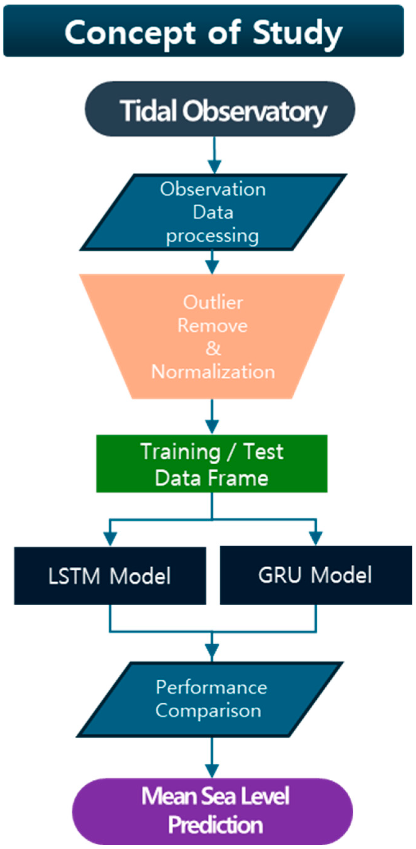
Figure 1. Conceptual workflow for mean sea level prediction: data collection, preprocessing (outlier removal, normalization), training/testing dataset creation, model training (LSTM, GRU), and performance comparison for optimal prediction.
Applsci 15 11067 g001
Figure 2. Location map and satellite image of Ulleungdo Island in the East Sea, about 120 km east of the Korean Peninsula, showing the study area for sea level trend analysis and the primary tide gauge observation site.
Applsci 15 11067 g002
Figure 3. LSTM unit showing forget, input, and output gates. Sigmoid (σ) and tanh activations control information flow, enabling the model to capture both short- and long-term dependencies.
Applsci 15 11067 g003
Figure 4. GRU architecture with reset and update gates controlling information flow for efficient long-term dependency modeling.
Applsci 15 11067 g004
Figure 5. Normalization scales all input features to the 0–1 range for model training, while inverse normalization verifies the accurate recovery of the original dataset.
Applsci 15 11067 g005
Figure 6. Training and validation results for mean sea level prediction in 2000 and Machine learning model performance for mean sea level prediction (2000–2021).
Applsci 15 11067 g006
Figure 7. Network architecture of the GRU-based sea level prediction model.
Applsci 15 11067 g007
Table 1. Summary of model parameters and training settings.
CategoryHyperParametersValues/SettingDescription
Data PreprocessingScale_cols‘MM’, ‘DD’, ‘hh’, Tide(cm)’Columns scaled using MinMaxScaler
window_size24Number of time steps in the input sequence (24 h)
feature_cols‘DD’, ‘hh’, Tide(cm)’Input features for the model
label_colsTide(cm)Target variable (output)
Model ArchitectureLSTM/GRU128Number of units in the LSTM/GRU layer
LSTM/GRU activation‘tanh’Activation function of the GRU layer
Dense activation‘linear’Activation function of the output layer
TrainingLoss function‘mse’Loss function (Mean Squared Error)
Optimizer‘adam’Optimizer used for training
Metrics[‘mse’]Metrics used to evaluate model performance
Epochs10Maximum number of training epochs
Batch size128Number of samples per gradient update
EvaluationMAECalculatedMean Absolute Error on test set
MSECalculatedMean Squared Error on test set
RMSECalculatedRoot Mean Squared Error on test set
R2CalculatedCoefficient of determination on test set
Table 2. Annual RMSE comparison between LSTM and GRU models from 2000 to 2018, including the overall average.
RMSE (cm)
LSTM
RMSE (cm)
GRU
R2
LSTM
R2
GRU
20000.03054830.03822240.938712510.91795243
20010.02677370.02354370.946830730.95923109
20020.01986610.01955910.938048170.94926756
20030.02380270.01545620.943825750.96688104
20040.02802770.01946040.940517360.95867230
20050.03321990.02414240.918316830.92986552
20060.01838070.01987620.942547760.95349526
20070.01875170.01855900.933613930.94880581
20080.02230060.02624480.936832140.93822615
20090.02210010.01662190.947558050.95272318
20100.02789980.01705300.937736570.95130882
20110.01902700.02089020.955123790.94951727
20120.02694340.01890830.940395620.95751103
20130.02038270.01921460.950656210.95301725
20140.02257110.01959380.942506730.95012517
20150.01828130.02171190.951781420.940106614
20160.03533170.02863140.931082830.93818435
20170.02345260.01961740.961270310.94774695
20180.03820110.01590210.916675170.96028611
Average0.02432950.02157930.940739610.94857567
Table 3. Statistical summary of predicted annual mean sea levels from 2018 to 2021 using the GRU model. The table includes the minimum, maximum, mean, and standard deviation (SD) of the predicted sea level values, along with the root mean square error (RMSE) for each year, indicating the model’s prediction accuracy relative to observed data.
YearMinMaxMeanSDRMSE (cm)R2
2018−33.421896870.1318895522.7902338915.55091620.4515157160.947321561
2019074.4218497933.1811876811.769264020.4243618790.956375532
2020−1.0004494477.0711394531.2258849310.419888220.4728188550.940678283
2021−10.035106285.5537728233.6119503415.068944620.4376743010.958148283
Disclaimer/Publisher’s Note: The statements, opinions and data contained in all publications are solely those of the individual author(s) and contributor(s) and not of MDPI and/or the editor(s). MDPI and/or the editor(s) disclaim responsibility for any injury to people or property resulting from any ideas, methods, instructions or products referred to in the content.