Simulation of Immiscible Counter-Current Flow in Porous Media Using a Modified Dynamic Pore Network Model

Abstract

Accurately simulating immiscible counter-current flow is crucial for applications from geological ${\mathrm{CO}}_2$ storage to shale gas production, yet it remains a major challenge for conventional pore network models (PNMs), which are unable to handle the numerical instability of opposing flows. To address this critical gap, we developed a novel dynamic PNM that incorporates a ‘transition state’ algorithm. This method successfully eliminates the spurious meniscus oscillations that hinder traditional models, enabling robust simulation of the complete counter-current process. Using this model, we quantify the profound impact of pore structure on flow efficiency. Our results demonstrate that increasing the pore size distribution uniformity (Weibull shape factor k from 0.5 to 3.0) extends the persistence of continuous air outflow pathways by more than six-fold (from 359 to over 2300 simulation steps). This leads to a quantifiable increase in the initial fluid exchange rate by nearly 10 times (from ${10}^{-11}$ to ${10}^{-10}$ ${\mathrm{m}}^3$/s) and a reduction in final residual air saturation by 53% (from 0.91 to 0.43). This work provides a tool for predicting and optimizing counter-current flow efficiency in subsurface engineering applications.

1. Introduction

Immiscible displacement in porous media is broadly classified by flow direction into co-current and counter-current regimes [1]. The former describes the parallel flow of wetting and nonwetting phases, while the latter involves the two phases flowing in opposite directions. Counter-current flow is the dominant mechanism in numerous critical applications, including flood irrigation, geological ${\mathrm{CO}}_2$ storage, and shale gas production, where the outflow path of the nonwetting phase is typically obstructed by the invading wetting phase. A fundamental understanding of the mechanisms controlling immiscible counterflow is therefore essential for optimizing irrigation design and enhancing recovery in gas/oil reservoirs [2,3,4]. As this process is governed by a complex interplay of capillary and viscous forces, pore-scale investigations are necessary to reveal its underlying displacement dynamics. However, the highly dynamic and unsteady nature of counterflow presents significant challenges for both experimental measurement and numerical simulation [1,5]. Consequently, the vast majority of existing studies have been constrained to the simpler case of co-current displacement, leaving a critical gap in predictive capabilities for many real-world scenarios.

It has been noticed in the literature that the architecture of a porous medium plays a critical role in governing immiscible displacement processes. Numerous studies, utilizing methods from field experiments to advanced micro-computed tomography (Micro-CT), have demonstrated that pore connectivity, size distribution, and macroporosity directly control key transport properties like hydraulic conductivity [6,7,8,9]. While various metrics have been proposed to quantify these structure–function relationships [10,11], the vast majority of this research has focused on co-current flow. Consequently, despite a broad consensus on the importance of pore structure [12,13,14,15], its specific influence on the dynamics of counter-current flow remains poorly understood, which hinders the development of predictive capabilities [16].

To investigate these unresolved mechanisms, physically based modeling is essential. While high-fidelity methods like the Lattice Boltzmann Method (LBM) can capture pore-scale physics in great detail, they are computationally prohibitive for the millimeter-to-centimeter-scale domains relevant to this study. In contrast, pore network models (PNMs), first introduced by Fatt [17], offer a compelling balance between computational efficiency and physical realism. By idealizing the pore space as a network of discrete pore and throat elements, PNMs can simulate displacement across large domains while retaining key mechanisms such as capillary effects, viscous forces, and topological connectivity. PNMs are broadly classified into quasi-static models, which neglect viscous forces and are suited to capillary-dominated regimes [18,19,20,21,22,23], and dynamic models that account for both capillary and viscous effects by solving for pressure fields [24,25,26,27,28,29,30]. The state of the art in dynamic PNMs has become highly sophisticated, as summarized in Table 1. Key advancements include the shift from computationally simpler single-pressure algorithms to more physically robust two-pressure methods that capture dynamic capillary effects within pores [31,32]. To address the high computational cost, adaptive/hybrid models have also been developed to efficiently combine dynamic and quasi-static algorithms [33].

Table 1. Comparison of dynamic pore network models for simulating counter-current flow.

Author(s)	Model Type	Pressure Algorithm	Key Physical & Algorithmic Features	Limitation for Counter-Current Flow
Blunt [19], Valvatne and Blunt [34]	Quasi-Static	N/A (Iterative on Pc)	Capillary-driven filling based on entry pressure thresholds.	Inherently static; neglects all dynamic and viscous effects.
Al-Gharbi and Blunt [28]	Dynamic	Single-Pressure	Film flow and snap-off in angular pores; viscous forces included.	Simplifies local physics; algorithm prohibits counter-flow.
Joekar-Niasar and Hassanizadeh [31]	Dynamic	Two-Pressure	Dynamic capillary effects, robust viscous coupling, non-equilibrium phenomena.	Focus on co-current flow; not designed for bulk counterflow.
Qin et al. [35]	Dynamic	Two-Pressure	Image-based; competition between arc menisci (AM) and main terminal menisci (MTM) filling.	Validated and designed exclusively for co-current spontaneous imbibition.
Regaieg and Moncorgé [33]	Adaptive/Hybrid	Single-Pressure (in dynamic zones)	High efficiency via adaptive switching between dynamic and quasi-static algorithms based on a physics-based criterion.	Explicitly states “counter-flow invasions are not considered”.
This Work	Dynamic	Single-Pressure (in dynamic zones)	Novel ‘two-motion’ algorithm enabling stable, simultaneous opposing flow. Viscous coupling and topological trapping in counterflow.	N/A (The first dynamic PNM capable of stably simulating immiscible counterflow without artificial restrictions).

However, despite these advancements, a fundamental limitation has confined the application of PNMs almost exclusively to co-current displacement. This stems from a critical numerical instability, often termed ’meniscus shaking’, which arises when modeling simultaneous, opposing flows. To circumvent this issue, the governing algorithms in virtually all existing dynamic PNMs—including advanced adaptive models—strictly prohibit menisci from moving against the bulk flow direction, a restriction explicitly acknowledged in the literature [33,35].

This study directly addresses this long-standing challenge by developing a novel dynamic pore network model specifically designed for simulating immiscible counter-current flow. The remainder of this paper is organized as follows. Section 2 details the methodology, including the construction of the pore networks and the formulation of the ‘two-motion’ algorithm designed for counter-current flow. Section 3 presents and discusses the simulation results, focusing on the impact of pore size distribution on flow patterns and efficiency in both 2-D and 3-D networks. Finally, Section 4 summarizes the key findings and conclusions of this study.

2. Materials and Methods

2.1. Pore Network Construction

To investigate the influence of pore structure heterogeneity, we first generated a series of two-dimensional (2-D) computational domains synthetically. This was accomplished using the open-source pore network modeling package OpenPNM [36]. Each synthetic network was constructed on a 20 mm × 20 mm domain and comprised a 50 × 50 grid of 2500 pores (Figure 1a). The diameters (d) of these pores were stochastically drawn from a Weibull probability distribution (Equation (1)), a function defined by a scale factor ($\lambda$) and a shape factor (k).

$$f(d;\lambda ,k)={\displaystyle \frac{k}{\lambda }}{\left({\displaystyle \frac{d}{\lambda }}\right)}^{k-1}{e}^{-{(d/\lambda )}^k}$$

(1)

In this formulation, $\lambda$ correlates with the mean pore diameter, while k governs the uniformity of the distribution. For this study, we systematically varied the shape factor k from 0.5 to 3.0, thereby creating a suite of networks with pore size distributions ranging from highly heterogeneous to increasingly uniform, as depicted in Figure 1b, with their coordination numbers equal to 3.92 and typical aspect ratios varying from 1.10 to 1.77.

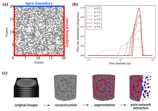
Figure 1. Pore networks used in this study: (a) 2-D synthetic network, (b) pore size distributions for varying shape factor k, and (c) 3-D network from Micro-CT (blue pixels: water, red pixels: air, gray pixels: solid).

In parallel, we conducted physical experiments using natural porous media, with the primary material being a water-wet natural silica sand (Accusand 30/40 grade, Unimin Corp., Ottawa, ON, Canada) characterized by a particle size of 0.60–0.85 mm and negligible organic content (<0.1 wt%). Prior to imaging, the sand was washed, dried at 45 °C, and packed into a 27 cm long acrylic cylinder (with a 2.9 cm inner diameter). This packed column was first scanned under dry conditions using a Hiscan XM Micro-CT system (Suzhou Hiscan Information Technology Co., Ltd., Suzhou, China). The acquisition parameters were set to 80 kV and 100 µA, with a 50 ms exposure and a 0.5° rotation step over 360°, yielding a resolution of 25 µm. Subsequently, a counter-current flow was established by injecting water from the top of the column. After 0.5 pore volumes of injection, the column was scanned again to capture the multiphase fluid distribution. Similar experiments were also performed on crushed silica sand and crushed limestone to broaden the scope of our observations.

The resulting stack of 2-D projection images was then processed. First, we performed 3-D volume reconstruction using the Visualization Toolkit (VTK), an open-source library for 3D graphics and image processing. To reduce computational cost, the reconstructed volumes were resampled to an isotropic resolution of 50 µm. The final stage of the workflow involved quantitative analysis using PoreSpy V1.3.1, a Python toolkit for porous media image analysis. The grayscale CT volumes exhibited a trimodal histogram, with distinct peaks for the solid, water, and air phases. This allowed for segmentation via a thresholding procedure calibrated to match the known porosity values exactly (0.34 for the natural silica sand). From the segmented image, a representative pore network (Figure 1c) was extracted using the SNOW algorithm implemented in PoreSpy. This algorithm identifies individual pores and allows for the determination of their equivalent spherical diameters, providing a direct link between the experimental system and our network modeling framework.

Based on the original 3-D network extracted from natural silica sand (which has the most uniform pore size distribution), the pore/throat diameter distributions are further skewed using the following equation to derive networks of different pore size distributions:

$$d^{\prime }=\left\{\begin{array}{cc}\overline{d}{\left({\displaystyle \frac{d}{\overline{d}}}\right)}^{1/k^{\prime }}\hfill & ,d<\overline{d}\hfill \\ \overline{d}{\left({\displaystyle \frac{d}{\overline{d}}}\right)}^{k^{\prime }}\hfill & ,d\ge \overline{d}\hfill \end{array}\right.$$

(2)

where $d^{\prime }$ is the skewed pore/throat diameter; d is the original pore/throat diameter; $\overline{d}$ is the mean original diameter; $k^{\prime }$ is the skewness coefficient; and the uniformity of pore size distribution decreases with the decrease in $k^{\prime }$.

The initial and boundary conditions for the counter-current simulations are defined to replicate a counter-current flow scenario. Initially, the entire pore network is saturated with the non-wetting phase (air) at a uniform pressure. The boundary conditions are then set as follows: the top boundary of the network is exposed to an infinite reservoir of the wetting phase (water) at a constant pressure ($P=P_{\mathrm{atm}}$). This open boundary allows for the infiltration of water driven by capillary forces, while simultaneously serving as the sole outlet for the displaced air. All other boundaries of the network are defined as no-flow (closed) boundaries, preventing any flux across them (as shown in Figure 1a). This setup ensures that the net flux across the system is zero and that fluid displacement is governed exclusively by the counter-current exchange at the open interface.

2.2. The Calculation Model

2.2.1. Governing Equations

After building the pore network, fluid flows are simulated and these are clearly governed by local pressure gradients: consequently, nodal pressures need to be computed in order to know how the fluids move over a given timestep. The pressure solver is based on the mass conservation equation. Simply, at node i, the flows going in and out are equal, so we can write

$$\sum _{j=1}^{N_i}{q}_{ij}=0$$

(3)

where N is the number of throats connected to the node, and $q_{ij}$ is the flow rate from node i to node j. In air–water two-phase flow, the flow within a pore situated at the interface separating wetting and nonwetting phases must account for the capillary pressure drop across that interface, and so for active menisci (i.e., the menisci that are not entrapped in the network), we now have

$$q_{ij}=\left\{\begin{array}{cc}{g}_{ij}(P_i-P_j-P_c)\hfill & ,P_i-P_j>P_c\hfill \\ 0\hfill & ,P_i-P_j\le P_c\hfill \end{array}\right.$$

(4)

where $g_{ij}$ is the conductance of the throat linking node i and node j, $P_c$ is the capillary entry pressure in the throat linking node i and node j, and $P_i$ and $P_j$ are the pressures at node i and node j, respectively. The capillary entry pressure $P_c$ is determined using a simple Young–Laplace law as follows:

$$P_c={\displaystyle \frac{2\gamma cos\theta }{r}}$$

(5)

where $\gamma$ is the surface tension of the fluid ($\gamma =0.072$ N/m in this study), $\theta$ is the contact angle ($\theta$ = 30° for the silica sand surface and dynamic contact angle is not considered in this study), and r is the radius of the throat. And the conductance $g_{ij}$ is determined using Poiseuille’s Law for a cylindrical throat element:

$$g_{ij}={\displaystyle \frac{\pi r_{ij}^4}{8\mu L_{ij}}}$$

(6)

where $r_{ij}$ is the radius of the throat linking node i and node j, $\mu$ is the viscosity of the fluid, and $L_{ij}$ is the length of the throat linking node i and node j.

The relative importance of gravitational to capillary forces is quantified by the dimensionless Bond number, $Bo$:

$$Bo={\displaystyle \frac{\Delta \rho g{r}^2}{\gamma }}$$

(7)

where $\Delta \rho$ is the density difference between the phases and g is the acceleration due to gravity. Using a characteristic length scale equivalent to the average throat radius ($r\approx 40$ µm), the Bond number for the simulated air–water system is calculated to be approximately $2\times {10}^{-4}$. Since $Bo\ll 1$, gravitational forces are negligible compared to capillary forces. Consequently, the effect of gravity is not included in the pressure calculations, and the orientation of the network relative to gravity is not a factor in this study.

2.2.2. The Scheme of the Dynamic Counterflow Model

In this study, a new dynamic counterflow pore network simulator is proposed to simulate the process of counterflow. The simulator is built upon an earlier dynamic pore network model developed by Regaieg and Moncorgé [33] for the simulation of the drainage process. Regaieg and Moncorgé’s model simplified the problem of immiscible displacement and pressures were simply derived using a pseudo-single-phase approach. However, as mentioned above, the description of menisci movement in these existing pore network models can lead to severe shaking during counterflow simulation. Thus significant modifications should be made to Regaieg’s model to simulate counterflow, and the simulation steps of the modified new model (Figure 2) are described as follows:

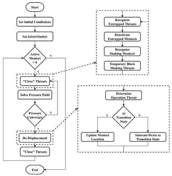
Figure 2. Flow chart for the proposed counterflow pore network model.

Step 1. The initial and boundary conditions are set. All the pores are initially filled with air and the initial pressure field is solved. In this study, the network boundaries are considered sealed, except for the water inlets and air outlets at the top boundary of the network. Thus, as water infiltrates into the network from top to bottom, the counter-current airflow forms naturally.

Step 2. A clustering technique is used to identify the active air clusters that are connected to the outlets. And the menisci between water clusters and active air clusters are considered active menisci. The active menisci should be larger than 0 for the following displacement events to be conducted.

Step 3. Based on the solved pressure field, the pressure gradients across the pores or throats are used to compute local flow rates that are subsequently used to determine the displacement events that control the movement of air–water menisci. An elaborately designed ‘two-motion’ algorithm is proposed here to update the menisci in each throat, making the simulation of counter-current menisci movements possible in the network (an important consideration when modeling the process of counterflow, which will be discussed in detail in the following section).

Step 4. After each displacement step, the clustering algorithm is conducted again and the entrapped menisci will be deactivated. Then steps 2–4 are repeated as long as active menisci exist in the network.

Step 5. Finally, the simulation halts when there are no active menisci in the network, with the pressure field in the network approaching a stable equilibrium state.

2.2.3. Time Integration Scheme

In this work, an explicit time-integration scheme is employed to update the fluid distribution over time. To ensure numerical stability and prevent non-physical overfilling, the simulation time-step, $\Delta t$, is dynamically controlled at every step. This is achieved by adopting a stability criterion analogous to a Courant–Friedrichs–Lewy (CFL) condition, which limits the time-step so that only the fastest-filling throat can be completely filled. The time-step is calculated as

$$\Delta t=C·\underset{ij}{min}\left({\displaystyle \frac{\Delta V_{ij}}{q_{ij}}}\right)$$

(8)

where $\Delta V_{ij}$ is the volume required to fill the throat connecting nodes i and j, $q_{ij}$ is the volumetric flow rate through it, and C is a safety factor (typically set to 1.0). This method ensures that at most one meniscus advances to a new pore in a single time-step, thus maintaining the stability of the explicit scheme. The locations of all other menisci are then updated based on their respective flow rates over this calculated $\Delta t$.

In addition, to verify that the simulation results are independent of the selected time-step size, a time-step convergence study was performed. The simulation for a representative network (k = 2.5) was conducted using the dynamically calculated time-step $\Delta t$ (from Equation (8) with C = 1.0), as well as with smaller time-steps of $0.5\Delta t$ and $0.1\Delta t$. As shown in Figure 3a, the resulting water saturation curves are visually indistinguishable, and the final residual air saturations differ by less than 0.1%. This demonstrates that our time-stepping scheme is convergent and the results are robust and reliable.

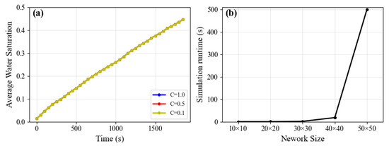
Figure 3. Model convergence and performance. (a) Water saturation evolution versus time under different control factors (C). (b) Simulation runtime under different network sizes.

2.2.4. The “Two-Motion” Algorithm for Stable Counter-Current Simulation

In conventional dynamic pore-network models, meniscus displacement is typically treated as a “one-motion” event: once a throat is selected for displacement, the meniscus immediately jumps from its current location to the next, and its capillary pressure abruptly changes from $P_{c1}$ to $P_{c2}$. This approach is effective for simulating pure drainage or imbibition processes where the flow is unidirectional. However, in counter-current flow simulations, this abrupt change is a major source of numerical instability.

As illustrated in Figure 4a,b, when a meniscus advances from a narrow throat (high capillary pressure $P_{c1}$) into a wider throat (low capillary pressure $P_{c2}$), the sudden drop in capillary pressure can instantly alter the local pressure gradient, often reversing its direction. This causes the meniscus to be immediately pushed back into the narrow throat in the subsequent time step, leading to non-physical “meniscus oscillations” between two or more throats and preventing the simulation from proceeding.

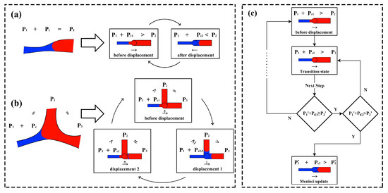
Figure 4. Schematics of (a,b) numerical meniscus shaking in conventional models and (c) the proposed ‘two-motion’ algorithm to resolve it.

To fundamentally resolve this issue, we propose a novel “two-motion” algorithm. The core idea is to decouple the displacement event from the meniscus location update by introducing a temporary “transition state” that allows for a physical check on the feasibility of the advance.

The algorithm is implemented as follows. For a meniscus poised for displacement, we define

• $\Delta P_{\mathrm{driving}}=P_w-P_{nw}$ as the driving pressure difference across the meniscus, where $P_w$ and $P_{nw}$ are the wetting and non-wetting phase pressures, respectively.
• $P_{c1}=2\sigma cos\theta /r_1$ as the capillary entry pressure of the throat $T_1$ where the meniscus currently resides, with $r_1$ being the throat radius.
• $P_{c2}=2\sigma cos\theta /r_2$ as the capillary entry pressure of the target throat $T_2$ that the meniscus is about to enter, with $r_2$ being the throat radius.

When a displacement event is triggered (i.e., $\Delta P_{\mathrm{driving}}>P_{c1}$), the throat is not immediately updated. Instead, it is flagged as being in a “transition state”. At the beginning of the next simulation step, the model checks all throats in the “transition state” and makes a decision based on the following precise mathematical conditions.

• Advance: If the driving pressure is sufficient to overcome the capillary barrier of the next throat, i.e., $\Delta P_{\mathrm{driving}}>P_{c2}$, the meniscus successfully advances. Its location is updated to the entrance of throat $T_2$, its capillary pressure is set to $P_{c2}$, and the “transition state” flag is removed.
• Pinning: If the driving pressure is insufficient to overcome the next capillary barrier (i.e., $P_{c1}<\Delta P_{\mathrm{driving}}\le P_{c2}$), or the meniscus is recognized as a “shaking” meniscus, then meniscus will be considered “pinned” or “blocked” in the pore between the current throat $T_1$ and the target throat $T_2$. Its physical location does not change, and its capillary pressure remains $P_{c1}$. The throat remains in the “transition state” until, in a future time step, the driving pressure $\Delta P_{\mathrm{driving}}$ increases sufficiently to meet the advance/retreat condition without shaking and then the meniscus can advance/retreat.
• Retreat: If, after entering the “transition state,” the local driving pressure reverses or decreases due to pressure changes elsewhere in the network such that $\Delta P_{\mathrm{driving}}\le P_{c1}$, the original displacement event is cancelled. The meniscus is released from the “transition state” and may undergo a retreat event within the current time step.

The pseudocode for this algorithm is presented in Algorithm 1.

Algorithm 1 The ‘two-motion’ algorithm for meniscus update,

Input: Set of all throats $T_{\mathrm{all}}$, set of throats in transition state $T_{\mathrm{trans}}$, pressure field P Output: Updated meniscus locations and throat states 1: while active menisci exist do              ▹ Main simulation loop 2:    Determine entrapped menisucs and shaking menisucs and block them 3:    Update pressure field P for the entire network and determine $\Delta t$                       ▹ Step 1: Identify new transitions 4:    for all active meniscus m not in $T_{\mathrm{trans}}$ do 5:       Calculate $\Delta P_{\mathrm{driving}}$ and $P_{c1}$ 6:       if $\Delta P_{\mathrm{driving}}>P_{c1}$ and $q\Delta t\ge \Delta V$ then 7:          Add throat of meniscus m to $T_{\mathrm{trans}}$          ▹ Enter transition state 8:       else if $\Delta P_{\mathrm{driving}}>P_{c1}$ and $q\Delta t<\Delta V$ then 9:          Update the location of the meniscus in the same throat 10:     end if 11:     end for                    ▹ Step 2: Process throats in transition state 12:     for all throat T in $T_{\mathrm{trans}}$ do 13:        Calculate current $\Delta P_{\mathrm{driving}}$ 14:        Identify target throat $T_{\mathrm{dest}}$ and calculate $P_{c2}$ 15:        if $\Delta P_{\mathrm{driving}}>P_{c2}$ then                  ▹ Case 1: Advance 16:           Update meniscus location to $T_{\mathrm{dest}}$ 17:           Remove T from $T_{\mathrm{trans}}$ 18:        else if $\Delta P_{\mathrm{driving}}\le P_{c1}$ then                ▹ Case 3: Retreat 19:           Remove T from $T_{\mathrm{trans}}$ 20:        end if     ▹ Case 2 (Pinning) is implicit: do nothing, T remains in $T_{\mathrm{trans}}$ 21:   end for 22: end while

2.2.5. Stability and Convergence Criteria

The numerical stability of this algorithm is an intrinsic property of its design. By introducing the “transition state” and its associated physical checks, the model converts non-physical, numerically induced oscillations into physically meaningful “pinning” events. This fundamentally avoids meniscus shaking and ensures a stable simulation. Under bounded pressure conditions, the algorithm ensures that a meniscus in the ‘pinning’ state will eventually either achieve the required driving pressure to advance into the neighboring pore or remain in place until it is entrapped. Since the total number of pores in the network is finite, and every element must ultimately be filled or become part of a trapped cluster, the algorithm is guaranteed to converge in finite time.

The convergence criterion for the simulation is defined as the point when no “active menisci” remain in the network. A meniscus is considered “active” if it is adjacent to a continuous, mobile non-wetting phase cluster (i.e., one connected to an outlet). When all non-wetting phase clusters become disconnected and trapped by the wetting phase, the set of active menisci becomes empty, the network reaches a hydrostatically stable equilibrium, and the simulation converges. This criterion for reaching equilibrium in the counter-current simulations is physically based and unambiguous. The simulation continues as long as there is a continuous path for the non-wetting phase (air) to be displaced and exit through the open boundary. Equilibrium is considered achieved when all remaining non-wetting phase clusters become disconnected from the outlet boundary, being fully encapsulated and hydrostatically trapped by the invading wetting phase (water). At this point, no further displacement is possible, and the simulation converges. Consequently, the saturation of the non-wetting phase reported at this final equilibrium state is the asymptotic residual saturation. This is distinct from an operational residual saturation, which is often defined by an arbitrary experimental duration or simulation time limit. Our physically based criterion ensures that the calculated residual saturation represents the true, maximum trapping capacity of the network under the given capillary-dominated conditions.

The computational performance of the model was evaluated on a standard desktop workstation. The cost increases non-linearly with the network size, primarily due to the growing size of the linear system of pressure equations solved at each timestep. As shown in Figure 3b, for a 2D network of 30 × 30 nodes, a typical simulation converges in approximately 1–2 s. However, for a 50 × 50 network, the simulation runtime increases significantly to 370–632 s. The total runtime is also proportional to the number of timesteps required to reach convergence; processes with smaller dynamic time-steps will require longer simulations. Given this computational scaling, direct simulation of field-scale problems is currently prohibitive. However, the model is ideally suited for its intended purpose as a digital rock physics tool to generate constitutive relationships.

3. Results and Discussion

As the ‘transition state’ of menisci movement is introduced to the model, the counter-current shaking of menisci is inhibited significantly. Thus, the new dynamic pore network model proposed in this study can be used for simulating immiscible counterflow for the first time. The morphology and evolution of counterflow patterns can then be depicted accurately according to the pore structure of the media. And the mechanisms controlling the process of counterflow can then be studied and discussed in detail.

3.1. Air–Water Counterflow Patterns in 2-D Networks of Different Pore Size Distributions

In order to investigate the effect of pore size distribution on the immiscible counterflow process, a series of counterflow simulations are carried out in 2-D artificial pore networks (Figure 5) and 3-D extracted pore networks (in Section 3.2). During simulation, both the inlets for water inflow and outlets for air outflow are set at the top boundary of the network, and pressures at the inlets and outlets are set to a constant of 1 atm. The patterns of air–water counterflow in 2-D networks of different pore size distributions are shown in Figure 5, with the infiltrating water phase shown in blue, and the outflowing air phase shown in red. It can be observed in Figure 5 that, at the very beginning of the counterflow infiltration (i.e., Figure 5(a1,b1,c1) when calculated steps = 50), the water infiltrates the network directly from the inlets at the top boundary; thus, finger-like infiltration patterns are observed. However, as the infiltration proceeds, the initial infiltration fingers tend to expand and merge with each other transversely due to capillary heterogeneity. Finally at the late stage of infiltration (Figure 5(a3,b3,c3)), clear displacement fronts develop in the network and piston-like infiltration patterns can be observed. Throughout the counterflow process, at least one continuous air outflow path survives in the network and extends from bottom to top to ensure the free expulsion of air phase. And if the air outflow paths are completely merged by the infiltrating water, the infiltration process will cease and the air phase at the bottom will be entrapped below the wetting front.

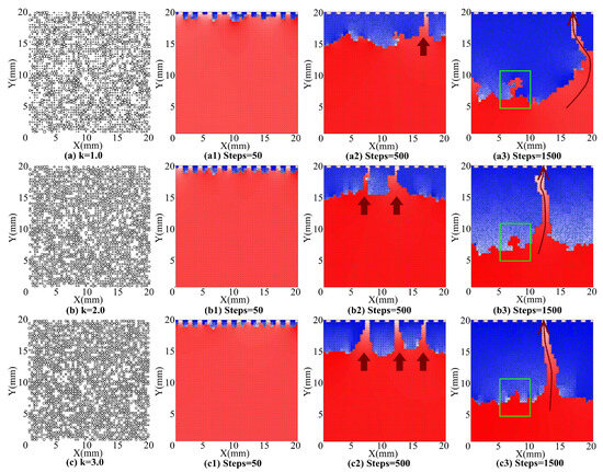
Figure 5. Air–water counterflow patterns in 2-D networks of different pore size distributions.

The number of simulated steps before infiltration ceases is summarized in Table 2. The simulated steps before infiltration ceasing varies under different pore size distributions—when the pore size distribution is quite heterogeneous (e.g., k = 0.5), the air outflow paths are merged quite quickly by the infiltrating water, and the simulation halts after only 359 steps, which means that the water only invades a small number of pores and a large amount of air is entrapped below the wetting front. And as the pore size distribution becomes increasingly uniform (e.g., k increases from 0.5 to 3.0), the number of time steps at which the simulation halts also increases from around 350 to around 2300, indicating that the air outflow paths survive for a longer time, and that a smaller amount of air is entrapped in the media. This suppression effect on path merging and air entrapment can also be observed in Figure 5. Comparing Figure 5(a2,b2,c2), it can be found that as the pore size distribution becomes more uniform, the transverse merging of infiltration fingers is suppressed, and thus more air outflow paths survive (three paths for k = 3.0 vs. one path for k = 1.0) after 500 steps of simulation. The suppression of transverse merging can be explained by the decrease in capillary heterogeneity—comparing the displacement pattern in the green rectangles in Figure 5(a3,b3,c3), it can be found that as the pore size distribution becomes more uniform, the displacement front becomes sharper and capillary absorption is obviously suppressed. As mentioned above, the transverse merging of infiltration fingers is mainly driven by capillary heterogeneity. Since the capillary heterogeneity is suppressed when the pore size distribution is uniform, the transverse merging is also suppressed and the air outflow survives for a longer time when k = 3.0.

Table 2. Simulation steps to convergence and final residual air saturation for 2-D networks with varying shape factor k.

k	0.5	1.0	1.5	2.0	2.5	3.0
Total Steps	359	1621	1773	1877	2343	2336
Residual air saturation	0.91	0.68	0.60	0.55	0.46	0.43

Furthermore, comparing the morphology of the air outflow path in Figure 5(a3,b3,c3), it can be found that as the pore size distribution becomes more uniform, the air outflow paths become straighter and broader. This air outflow path morphology should surely influence the inflow/outflow rate—as the air outflow path becomes increasingly straight and broad when the pore size distribution becomes more uniform, the air flows out more easily and the rate of initial air outflow increases by nearly 10 times (from ${10}^{-11}$ to ${10}^{-10}$ ${\mathrm{m}}^3$/s) as a result (Figure 6). With the increase in k, the residual air saturation also shows a decrease of 53% (from 0.91 to 0.43), as shown in Table 2.

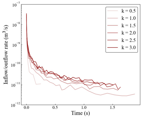
Figure 6. Inflow/outflow rate versus time for 2-D networks.

3.2. Air–Water Counterflow Patterns in 3-D Networks of Different Pore Size Distributions

Figure 7a–c shows the air–water counterflow patterns in 3-D networks of different pore size distributions. It can be seen in Figure 7c that when the pore size distribution is relatively uniform, the air outflow paths are highly dispersed, occupying a significant portion of the network above the wetting front. Conversely, as the pore size uniformity decreases (Figure 7a), the air outflow paths become more concentrated and are more easily merged by water due to increased capillary heterogeneity within the network. A similar phenomenon is also evident in the column slices of different media (Figure 7d–f). For media with relatively uniform pore size distributions (e.g., natural silica sand in Figure 7f), air clusters remain dispersed. In contrast, as pore size uniformity decreases, air clusters concentrate within the largest pores, resulting in less dispersed air outflow paths (e.g., crushed limestone in Figure 7d).

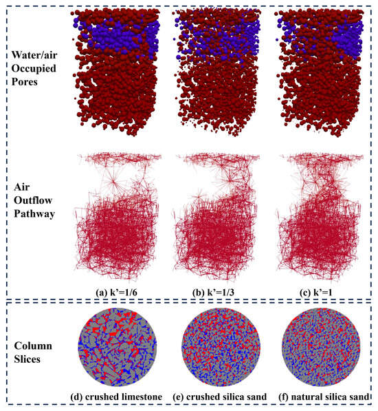
Figure 7. Simulated (a–c) and experimental (d–f) air–water distribution in 3-D pore networks.

To provide a more robust, quantitative validation, we directly compared the final residual air saturation distribution from our simulation with experimental results from micro-CT imaging (Figure 8). Given the highly dynamic nature of the counterflow process, capturing an accurate snapshot of the entire column via micro-CT is challenging due to the long scan times required. We therefore focused the comparison on the top 0–5 mm of the medium, where a stable residual state is established after the counterflow ceases. This approach provides a well-defined and static experimental target for validation. A point-by-point comparison between the slice average saturation values of the simulation and the experiment yields a coefficient of determination (R²) of 0.49 and a Mean Absolute Error (MAE) of 3%. Given the inherent stochastic nature of multiphase flow and the necessary idealizations in any pore network representation, a perfect point-by-point match is not expected. The benchmark study by Raeini et al. [37] suggests that a mismatch in average saturation of less than 10% represents “good accuracy” for two-phase PNM model validation against micro-CT data. Thus the MAE of 3% for the top 0–5 mm of the medium can be considered a good result in this context, confirming the model’s validity in capturing the macroscopic trends and spatial distribution of fluid trapping. The deviations observed in the point-by-point comparison (reflected by the R² value) can be attributed to several sources of uncertainty, including the network extraction algorithm’s approximation of the complex pore geometry, the model’s simplifying assumption of uniform wettability, and the fundamental randomness with which specific pathways are ultimately trapped.

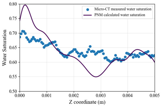
Figure 8. Comparison of Micro-CT-measured and PNM-calculated water saturation profiles.

The simulated inflow/outflow rate and air cluster connectivity in 3-D networks of different pore size distributions are shown in Figure 9. It can be found in Figure 9a that, similar to the 2-D conditions, the inflow/outflow rate in 3-D networks decreases with time and increases as the pore size distribution becomes more uniform. The decrease in the inflow/outflow rate with time can be attributed to the increase in flow resistance—as infiltration proceeds, the air outflow paths continue to merge, and the distance from water inlets to the wetting front also lengthens. Thus, the resistance of both the water inflow and air outflow increases, leading to the inflow/outflow rate decreasing with time. Meanwhile, the increase in inflow/outflow rate with $k^{\prime }$ can be attributed to the decrease in air outflow resistance, similarly to the 2-D conditions.

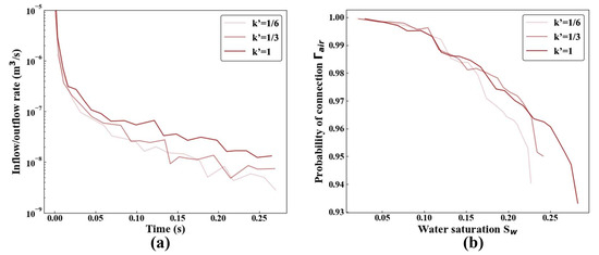
Figure 9. (a) Inflow/outflow rate versus time and (b) air cluster connectivity versus water saturation.

The connectivity of the air cluster in the pore space, denoted ${\Gamma }_{air}$, can be calculated using the following equation:

$$\Gamma ={\displaystyle \frac{1}{n_S^2}}\sum _{i=1}^N{n}_i^2$$

(9)

where $n_S$ is the total number of cells occupied by the air phase and $n_i$ is the number of cells within air cluster i. N is the total number of air clusters. $\Gamma$ is in fact the second-order moment of the distributions of the air clusters, and is referred to in the literature as “second geobody connectivity” or the “global connectivity index”. As shown in Figure 9b, the air cluster connectivity increases with increasing $k^{\prime }$, which means that as the pore size distribution becomes more uniform, capillary trapping is suppressed and fewer isolated air clusters are entrapped in the network. Since the entrapped air clusters act as barriers for water inflow, having fewer entrapped air clusters will directly lead to smaller water inflow resistance. Generally speaking, the change in the inflow/outflow rate under 3-D conditions can also be attributed to the change in flow resistance—the water inflow/air outflow resistance increases with time, but decreases as the pore size distribution becomes more uniform.

4. Conclusions

In this study, a new dynamic pore network model was successfully developed to simulate the counter-current flow of two immiscible phases. By incorporating a ‘transition state’ into the displacement algorithm, the model effectively overcomes the numerical meniscus oscillations that hindered previous simulations. Our 2-D simulation results provide a clear, quantitative link between pore structure and flow efficiency: as the pore size distribution becomes more uniform, the capillary heterogeneity is suppressed, allowing air outflow paths to persist for longer and adopt straighter, broader morphologies. Consequently, the initial inflow/outflow rate is enhanced by nearly an order of magnitude, and the final residual air saturation is reduced by 53%. Similar phenomena were qualitatively observed in 3-D simulations, confirming that a uniform pore structure is critical for efficient counter-current exchange.

In essence, this work presents the first dynamic pore-network model capable of stably simulating the complete immiscible counter-current flow process without imposing the artificial restrictions that have limited previous dynamic models. This breakthrough offers a robust predictive tool for subsurface engineering applications. In the context of geological ${\mathrm{CO}}_2$ sequestration, for example, the model allows engineers to predict storage efficiency and final residual gas saturation based on the pore structure of a potential site. This facilitates the early-stage identification of sites with more uniform pore distributions and higher storage capacity, ultimately improving sequestration security and economic viability, and preventing costly field tests at suboptimal locations. Furthermore, the framework’s generalizability extends readily to other domains mentioned, such as enhanced oil recovery, shale gas recovery, and agricultural irrigation. Simulating these systems is a matter of adapting key input parameters: for oil recovery, one would adjust the viscosity and density ratios to match the oil–brine system and modify the contact angle ($\theta$) to reflect reservoir wettability.

It should also be mentioned that the current model relies on several key simplifications. Specifically, it assumes a uniform wettability with a constant contact angle and idealized pore geometry, thus neglecting the effects of contact angle hysteresis on trapping events like snap-off. This simplification is particularly significant for applications such as geological ${\mathrm{CO}}_2$ storage in saline aquifers. In such systems, the dissolution of ${\mathrm{CO}}_2$ into brine forms a weak carbonic acid, which can react with the rock matrix over time, leading to dynamic wettability alteration. The assumption of a constant contact angle therefore fails to capture these long-term geochemical effects on fluid–rock interactions. Furthermore, neglecting contact angle hysteresis, a key mechanism for capillary trapping in the mixed-wet systems typical of reservoirs, likely leads to an underestimation of the ultimate residual ${\mathrm{CO}}_2$ saturation. Capturing these complex phenomena is crucial for accurately predicting the long-term security and trapping efficiency of ${\mathrm{CO}}_2$ sequestration. Moreover, the model omits phase interference mechanisms such as corner film flow, which limits its primary validity to capillary-dominated processes. Future work should therefore focus on incorporating these more complex physics to improve quantitative accuracy and extend the model’s applicability to mixed-wet systems and film flow-dominated scenarios. Furthermore, a thorough sensitivity and uncertainty analysis of key parameters will be a crucial next step in the future application of this model for quantitative predictions.

References

- Shad, S.; Gates, I. Multiphase flow in fractures: Co-current and counter-current flow in a fracture. J. Can. Pet. Technol. 2010, 49, 48–55. [Google Scholar] [CrossRef]
- Luckins, E.K.; Oliver, J.M.; Please, C.P.; Sloman, B.M.; Van Gorder, R.A. Modelling and analysis of an endothermic reacting counter-current flow. J. Fluid Mech. 2022, 949, A21. [Google Scholar] [CrossRef]
- Andersen, P.Ø. Early-and late-time prediction of counter-current spontaneous imbibition, scaling analysis and estimation of the capillary diffusion coefficient. Transp. Porous Media 2023, 147, 573–604. [Google Scholar] [CrossRef]
- Jaritsch, D.; Holbach, A.; Kockmann, N. Counter-current extraction in microchannel flow: Current status and perspectives. J. Fluids Eng. 2014, 136, 091211. [Google Scholar] [CrossRef]
- Chang, Y.; Shang, Q.; Sheng, L.; Deng, J.; Luo, G. Gas-liquid countercurrent flow characteristics in a microbubble column reactor. Chem. Eng. Sci. 2024, 300, 120573. [Google Scholar] [CrossRef]
- Rabot, E.; Wiesmeier, M.; Schlüter, S.; Vogel, H.J. Soil structure as an indicator of soil functions: A review. Geoderma 2018, 314, 122–137. [Google Scholar] [CrossRef]
- Pagliai, M.; Vignozzi, N. The soil pore system as an indicator of soil quality. Adv. GeoEcol. 2002, 35, 69–80. [Google Scholar]
- Paradelo, M.; Katuwal, S.; Moldrup, P.; Norgaard, T.; Herath, L.; De Jonge, L.W. X-ray CT-derived soil characteristics explain varying air, water, and solute transport properties across a loamy field. Vadose Zone J. 2016, 15, 1–13. [Google Scholar] [CrossRef]
- Sandin, M.; Koestel, J.; Jarvis, N.; Larsbo, M. Post-tillage evolution of structural pore space and saturated and near-saturated hydraulic conductivity in a clay loam soil. Soil Tillage Res. 2017, 165, 161–168. [Google Scholar] [CrossRef]
- Dexter, A.R.; Czyż, E.A. Soil physical quality and the effects of management. In Soil Quality, Sustainable Agriculture and Environmental Security in Central and Eastern Europe; Springer: Dordrecht, The Netherlands, 2000; pp. 153–165. [Google Scholar]
- Dexter, A.R. Soil physical quality: Part I. Theory, effects of soil texture, density, and organic matter, and effects on root growth. Geoderma 2004, 120, 201–214. [Google Scholar] [CrossRef]
- Naveed, M.; Moldrup, P.; Schaap, M.G.; Tuller, M.; Kulkarni, R.; Vogel, H.J.; de Jonge, L. Prediction of biopore-and matrix-dominated flow from X-ray CT-derived macropore network characteristics. Hydrol. Earth Syst. Sci. 2016, 20, 4017–4030. [Google Scholar] [CrossRef]
- Blunt, M.J. Multiphase Flow in Permeable Media; Cambridge University Press: Cambridge, UK, 2017; pp. 32–35. [Google Scholar]
- Hirmas, D.R.; Giménez, D.; Nemes, A.; Kerry, R.; Brunsell, N.A.; Wilson, C.J. Climate-induced changes in continental-scale soil macroporosity may intensify water cycle. Nature 2018, 561, 100–103. [Google Scholar] [CrossRef] [PubMed]
- Romero-Ruiz, A.; Linde, N.; Keller, T.; Or, D. A review of geophysical methods for soil structure characterization. Rev. Geophys. 2018, 56, 672–697. [Google Scholar] [CrossRef]
- Wei, Y.; Chen, K.; Wu, J. Estimation of the critical infiltration rate for air compression during infiltration. Water Resour. Res. 2020, 56, e2019WR026410. [Google Scholar] [CrossRef]
- Fatt, I. The network model of porous media. Trans. AIME 1956, 207, 144–181. [Google Scholar] [CrossRef]
- McDougall, S.R.; Sorbie, K.S. The impact of wettability on waterflooding: Pore-scale simulation. SPE Reserv. Eng. 1995, 10, 208–213. [Google Scholar] [CrossRef]
- Blunt, M.J. Pore level modeling of the effects of wettability. SPE J. 1997, 2, 494–508. [Google Scholar] [CrossRef]
- Oren, P.E.; Bakke, S.; Arntzen, O.J. Extending predictive capabilities to network models. SPE J. 1998, 3, 324–336. [Google Scholar] [CrossRef]
- Ryazanov, A. Pore Scale Network Modelling of Residual Oil Saturation in Mixed-Wet Systems. Ph.D. Thesis, Heriot-Watt University, Edinburgh, UK, 2012. [Google Scholar]
- Raoof, A.; Hassanizadeh, S.M. A new formulation for pore-network modeling of two-phase flow. Water Resour. Res. 2012, 48, W01514. [Google Scholar] [CrossRef]
- Li, J.; McDougall, S.R.; Sorbie, K.S. Dynamic pore-scale network model (PNM) of water imbibition in porous media. Adv. Water Resour. 2017, 107, 191–211. [Google Scholar] [CrossRef]
- Aker, E.; Måløy, K.J.; Hansen, A.; Batrouni, G.G. A two-dimensional network simulator for two-phase flow in porous media. Transp. Porous Media 1998, 32, 163–186. [Google Scholar] [CrossRef]
- Mogensen, K.; Stenby, E.H. A dynamic two-phase pore-scale model of imbibition. Transp. Porous Media 1998, 32, 299–327. [Google Scholar] [CrossRef]
- Hughes, R.G.; Blunt, M.J. Pore scale modeling of rate effects in imbibition. Transp. Porous Media 2000, 40, 295–322. [Google Scholar] [CrossRef]
- Singh, M.; Mohanty, K.K. Dynamic modeling of drainage through three-dimensional porous materials. Chem. Eng. Sci. 2003, 58, 1–18. [Google Scholar] [CrossRef]
- Al-Gharbi, M.S.; Blunt, M.J. Dynamic network modeling of two-phase drainage in porous media. Phys. Rev. E 2005, 71, 16308. [Google Scholar] [CrossRef]
- Nguyen, V.H.; Sheppard, A.P.; Knackstedt, M.A.; Pinczewski, W.V. The effect of displacement rate on imbibition relative permeability and residual saturation. J. Pet. Sci. Eng. 2006, 52, 54–70. [Google Scholar] [CrossRef]
- Aghaei, A.; Piri, M. Direct pore-to-core up-scaling of displacement processes: Dynamic pore network modeling and experimentation. J. Hydrol. 2015, 522, 488–509. [Google Scholar] [CrossRef]
- Joekar-Niasar, V.; Hassanizadeh, S.M. Effect of fluids properties on non-equilibrium capillarity effects: Dynamic pore-network modeling. Int. J. Multiph. Flow 2011, 37, 198–214. [Google Scholar] [CrossRef]
- Thompson, K.E. Pore-scale modeling of fluid transport in disordered fibrous materials. AIChE J. 2002, 48, 1369–1389. [Google Scholar] [CrossRef]
- Regaieg, M.; Moncorgé, A. Adaptive dynamic/quasi-static pore network model for efficient multiphase flow simulation. Comput. Geosci. 2017, 21, 795–806. [Google Scholar] [CrossRef]
- Valvatne, P.H.; Blunt, M.J. Predictive pore-scale modeling of two-phase flow in mixed wet media. Water Resour. Res. 2004, 40, W07406. [Google Scholar] [CrossRef]
- Qin, C.Z.; van Brummelen, H.; Hefny, M.; Zhao, J. Image-based modeling of spontaneous imbibition in porous media by a dynamic pore network model. Adv. Water Resour. 2021, 152, 103932. [Google Scholar] [CrossRef]
- Gostick, J.; Aghighi, M.; Hinebaugh, J.; Tranter, T.; Hoeh, M.A.; Day, H.; Spellacy, B.; Sharqawy, M.H.; Bazylak, A.; Burns, A.; et al. OpenPNM: A pore network modeling package. Comput. Sci. Eng. 2016, 18, 60–74. [Google Scholar] [CrossRef]
- Raeini, A.Q.; Yang, J.; Bondino, I.; Bultreys, T.; Blunt, M.J.; Bijeljic, B. Validating the generalized pore network model using micro-CT images of two-phase flow. Transp. Porous Media 2019, 130, 405–424. [Google Scholar] [CrossRef]
Disclaimer/Publisher’s Note: The statements, opinions and data contained in all publications are solely those of the individual author(s) and contributor(s) and not of MDPI and/or the editor(s). MDPI and/or the editor(s) disclaim responsibility for any injury to people or property resulting from any ideas, methods, instructions or products referred to in the content. |
© 2025 by the authors. Licensee MDPI, Basel, Switzerland. This article is an open access article distributed under the terms and conditions of the Creative Commons Attribution (CC BY) license (https://creativecommons.org/licenses/by/4.0/).