Data Analysis of Two-Vehicle Accidents Based on Machine Learning

Featured Application

This study analyzes two-vehicle accident data using machine learning and avoids the variable covariance problem through factor analysis, which provides new ideas for related research. Meanwhile, clustering results provide a reference for automatic driving test scenarios and standardization.

Abstract

Road traffic accidents are the eighth leading cause of human deaths. In order to study two-vehicle accidents, this paper extracted data from 493 two-vehicle accidents from the CIDAS database from 2011 to 2022, used machine learning methods to analyze the accident data, and obtained the significance of two-vehicle accident parameters. Finally, five typical scenarios of two-vehicle accidents were obtained based on this. The results of the significance analysis show that vehicle parameters have a greater impact on occupant injury in the host vehicle; clustering results show that lighting, the number of lanes, the other vehicle’s type, and the speed of the host vehicle have a large impact on occupant injury (for example, the injury rate for the high-speed, nighttime Scenario II was 52.9%, compared to just 10.9% for the lower-speed Scenario IV). Factor analysis results show that precipitation has a large impact on occupant injury, as the frequency of injuries in rainy conditions was 13.4% higher, and the frequency of serious injuries was 7.9% higher, than in accidents without rain. This paper innovatively uses factor analysis to reduce the dimensionality of categorical variables, which provides research ideas for related research. At the same time, the clustering results obtained in this paper also provide references for the establishment of corresponding test scenarios for autonomous driving and the establishment of standards.

1. Introduction

With the increase in car ownership, the rate of traffic accidents is also increasing [1]. The World Health Organization reports that road traffic injuries are the eighth leading cause of death [2]. Therefore, conducting automobile safety research is crucial for improving road safety.

Currently, automotive safety research is mainly categorized into passive safety and active safety research methods. Among them, along with the rapid development of sensor technology and machine learning algorithms, etc., automobile active safety technology has made significant progress in recent years. Automotive active safety technology can take warning and auxiliary control of the vehicle in typical accident scenarios to reduce the intensity of the accident or avoid the occurrence of an accident. However, the current research on active safety accident scenarios is dominated by motor vehicle interaction scenarios with vulnerable road users, and relatively little research has been conducted on conflict scenarios between motor vehicles.

Zhou et al. [3] conducted clustering analysis of NAIS crash data to identify six typical car-two-wheeler scenarios. These were reconstructed in Prescan to simulate AEB performance and optimize sensor configurations under varying conditions. However, the study did not specify whether multicollinearity among accident variables had been addressed before the cluster analysis. Directly applying cluster algorithms to high-dimensional, highly correlated data may lead to biased or unstable scenario definitions.

Sujayanont et al. [4] used multiple logistic regression to analyze injury surveillance data from Khon Kaen, Thailand. Their study identified common gender, older age, alcohol consumption, and nighttime driving as significant risk factors increasing the likelihood of severe traffic accident outcomes. Nevertheless, the limited number of variables available for selection during the research process may also be one of the reasons for the low specificity of the predictive model.

Wahab et al. [5] applied several machine learning models to predict motorcycle crash severity, identifying key contributing factors. However, their study did not explore a broader range of machine learning techniques or conduct more in-depth data analysis, which may limit the generalizability and robustness of the findings.

Wu et al. [6] proposed a random parameter multinomial Logit model with heterogeneous means and variances, conducting a detailed analysis of the differences in risk factors across various types of two-vehicle collisions and successfully capturing changes in model parameters caused by unobserved factors. This method demonstrates significant advantages in addressing “unobserved heterogeneity.” However, it is necessary to incorporate more extensive and diverse two-vehicle collision datasets and minimize the impact of deficiencies inherent in the original data.

Muhammad Ijaz et al. [7] analyzed the injury severity of tricycles using various machine learning algorithms, such as decision tree (DT), random forest (RF), and decision jungle (DJ). Furthermore, they determined the significance ratings of each attribute through a feature importance assessment based on random forest, which used the occupant injury value as the target variable. Although the models used in the study are highly interpretable, analysis of other datasets may require the use of cutting-edge models such as deep learning.

This paper combines the requirements of the project for the analysis of two-vehicle accidents. Firstly, after a general preview of the accident data, ML (Machine learning) methods such as DT and RF were used to process the accident data and the parameter significance of the variables were obtained because the covariance between the variables was not eliminated, which would affect the results of the subsequent clustering. The choice was made to use the results obtained by factor analysis to perform a dimensionality reduction to reduce the multivariate covariance of the variables, making the clustering results more accurate. After reducing dimensionality through factor analysis, we clustered the cases using a Euclidean distance metric to identify typical two-vehicle accident scenarios.

2. Materials and Methods

The database used in this study is the CIDAS (China In-Depth Accident Study) database. A total of 493 accident cases were extracted, and the sampling criteria of the database cases in this paper are as follows:

The accidents occurred between 2011 and 2022, and each case involved only two motor vehicles.

Drawing on previous research [8,9,10,11], we chose to extract the parameters shown in Figure 1.

2.1. Non-Public Parameters

2.1.1. Continuous Variables

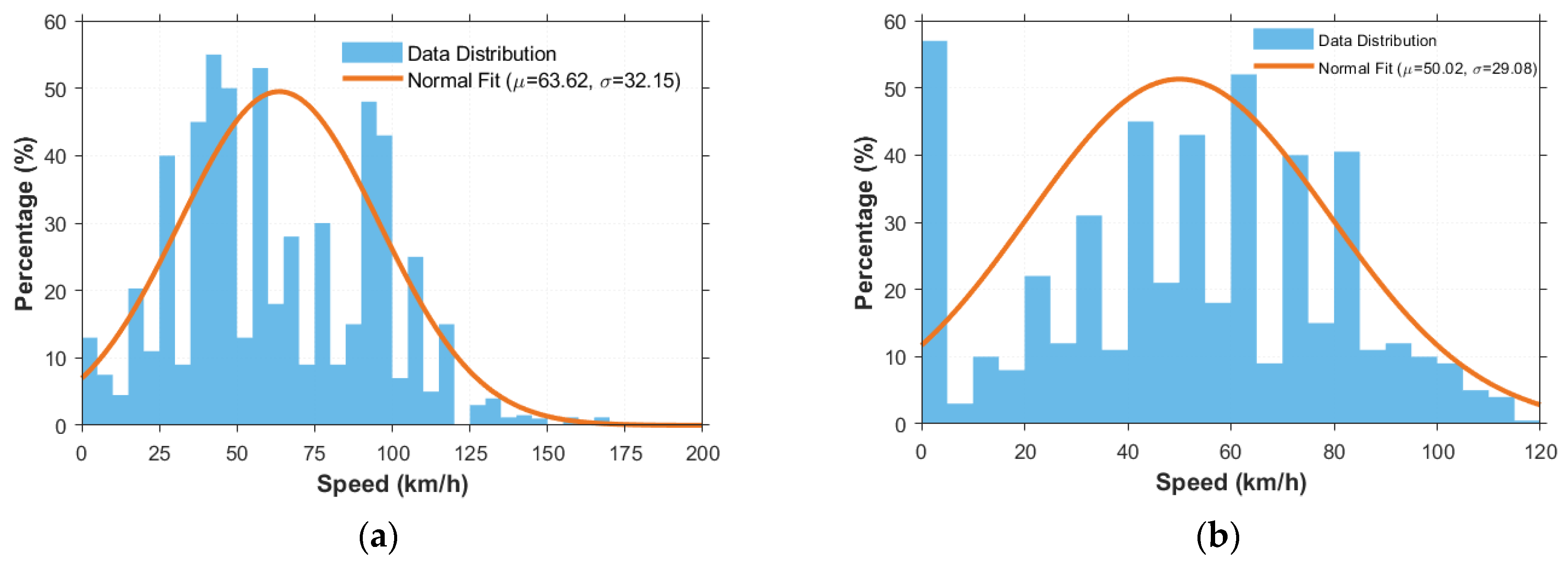
Among the extracted data, only speed is a continuous variable. The speed bar graphs of car A and car B, and their fitted normal curves, are shown in Figure 2. The mean value of the fitted normal curve for the speed of car A is 63.62, and the standard deviation is 32.15; the mean value of the fitted normal curve for the speed of car B is 50.02, and the standard deviation is 29.08. Public (lighting, precipitation, time of day, road surface and condition, lanes, visibility, road class, on-site road environment, accident pattern) and non-public (A/B vehicle type, steering, injury, speed) parameters were selected from CIDAS fields based on coverage, scenario describability, and ML-based importance for 493 cases. Speed ranges and step sizes follow the empirical modes in Figure 2 and Euro NCAP increments; lighting levels follow IVISTA; lane widths and markings follow national design codes and C-NCAP/ISO provisions.

Combined with the CIDAS data description, this paper specifies that vehicle A is the main vehicle of the accident, which is the main object of the study, and vehicle B is the participating vehicle, which is mainly considered based on the effect of its accident parameters on the injury of occupants of the main vehicle.

2.1.2. Classification Variables

For the non-public parameters of vehicle A and vehicle B, these are their respective car models, occupant injuries, and steering types, which are detailed in

Table 1. Non-public parameters.

Vehicle Type	Number of A Cases	Number of B Cases	Personnel Injuries	Number of Injuries in Vehicle A	Number of Injuries in Vehicle B	Steering Type	Number of A Cases	Number of B Cases
Car	414	333	No injuries	277	320	No steering	291	319
Trucks	69	146	Minor injuries	132	114	Left turn	84	59
Bus	10	14	Serious injuries	34	32	Right turn	61	61
Total	493	493	Deaths	50	20	Right lane change	17	18
			Total	493	486	Not applicable	13	9
						Left lane change	11	7
						Unknown	16	20
						Total	493	493

.

The main vehicle types in the accidents were all cars, with the smallest percentage of passenger cars and almost twice as many trucks in B as in A.

Regarding occupant injuries, there are no missing cases in A and seven missing cases in B. Most double motor vehicle accidents involve only vehicle damage, with occupant injuries mainly being either no injuries or minor injuries. However, serious injuries and fatalities accounted for 17% of the total cases for A and about 10% for B, which is significantly lower.

All types of steering maneuvers were included, but there were undefined values in the database (12 for Class A and 17 for Class B). These were classified as “unknown” and were not used in the data analysis, similar to the “not applicable” category, which together accounted for 6% of the total. No steering maneuvers accounted for 60% of all accidents, followed by cases involving steering maneuvers, while lane change cases were the least numerous.

2.2. Common Parameters

None of the public parameters shown in

Table 2. Public parameters.

Parameter	Parameter Values	Number of Cases
Street light status	No street lights	218
	Street lights off	173
	Street lights on	102
Precipitation condition	No	442
	Rain	41
	Snow	10
Time of day	Daytime	286
	Evening	162
	Dusk	45
Road surface	Good	434
	Other	30
	Potholes	29
Road surface condition	Dry	394
	Damp	33
	Wet	37
	Snow-covered	21
	Icy	7
	Other	1
Number of lanes in the direction of travel	1	120
	2	203
	3	119
	4	39
	5	9
	6	3
Visibility	No fog	486
	<2000 m	3
	<100 m	1
	<200 m	1
	<500 m	1
	<1000 m	1
Road classification	Other	174
	National highway	96
	County road	77
	High speed	73
	Provincial road	44
	Township road	29
On-site road environment	Straight	230
	Cross intersection	118
	General intersection	99
	Curve	39
	Roundabouts	2
	Ramp	2
	Gated intersections	1
	Other	2
Accident pattern	Side impact	213
	Rear-end collision	146
	Head-on collision	56
	Collision with parked vehicle	32
	Same-direction sideswipe	29
	Collision with fixed object	8
	Opposite-direction sideswipe	5
	Multi-vehicle collision	2
	Other	2

were missing.

Across all cases, there were 102 cases in which street lights were turned on; combining the following time periods, 162 cases at night and 45 cases at dusk, for a total of 207 cases, half the cases occurring in the poorly illuminated night or dusk featured street lights which were not turned on. The rest of the nearly 300 accidents occurred during the daytime.

No precipitation conditions accounted for the vast majority of accidents. Roadway conditions, road surface, and fog visibility showed similar trends.

The number of lanes in the direction of roadway travel was dominated by 1, 2, and 3 lanes. The five types of roads—“national highways”, “county highways”, “provincial highways”, “rural highways”, and “high speed”—were the same. “Highways” accounted for two-thirds of the total number of cases, with little difference between them.

The road environment at accident sites was characterized by a mix of “straight roads”, “intersections”, “crossroads”, and “curves”.

In terms of accident patterns, side collisions and rear-end collisions accounted for nearly 70% of the accidents; front collisions, collisions with stationary cars, and same-direction scraping accounted for about 24%; other types of accidents made up only a very small proportion and were not typical.

The traffic volume of the accident sections defined in the database was less than the traffic volume, so they were not put into the table for display.

3. Machine Learning-Based Dangerous Scenario Analysis

The severity of traffic accident injuries results from the interaction of multiple factors [7]. Significance analysis of accident parameters helps identify the main causes of accidents. It also aids in replicating accident scenarios to differentiate responsibility or to develop dangerous scenario simulations.

3.1. Data Preprocessing

Data preprocessing included parameter extraction, format harmonization, polarity alignment, and feature scaling [12].

For variables with a clear physical order (e.g., lighting, precipitation, road surface condition, visibility, traffic flow), we applied a monotonic [0, 1] scoring with “more adverse = higher score,” followed by standardization.

Purely nominal variables without an inherent order (e.g., B vehicle type, collision pattern, maneuver/turning type) were one-hot encoded for the clustering stage and were not assigned artificial ranks. To balance feature scales and avoid any single feature range dominating distance calculations, we standardized continuous and scored variables (z-score); one-hot features were kept in {0,1}.

3.2. Significance Analysis

The primary objective of this stage was to identify typical accident scenarios through cluster analysis. However, accident datasets are often characterized by high dimensionality and multicollinearity, where numerous variables are interrelated. Applying distance-based clustering algorithms directly to such data can lead to biased or unstable results, as groups of correlated variables can disproportionately influence the outcome. To address this, a two-step approach was adopted. First, factor analysis was employed to reduce the dimensionality of the data and transform the correlated variables into a smaller set of uncorrelated latent factor dimensions. Second, cluster analysis was performed on the resulting factor scores. This ensured that the scenarios were grouped based on uncorrelated underlying dimensions, leading to more robust and interpretable results.

3.2.1. Factor Analysis

Factor analysis was used to analyze the data. The factor analysis model can be expressed as follows:

$$X=M+L·F+ϵ,$$

(1)

where X is the observation matrix, M is the mean matrix, L is the factor loading matrix, F is the factor matrix, and ϵ is the error term matrix.

To verify applicability, the KMO and Bartlett tests were used:

$$\mathrm{K}\mathrm{M}\mathrm{O}={\displaystyle \frac{\sum _i\sum _{i\ne j}{r}_{ij}^2}{\sum _i\sum _{i\ne j}{r}_{ij}^2+\sum _i\sum _{i\ne j}{p}_{ij}^2}},$$

(2)

$${\chi }^2=-\left(n-1-{\displaystyle \frac{2p+5}{6}}\right)\mathrm{l}\mathrm{o}\mathrm{g}|R|,$$

(3)

where r_ij is the correlation coefficient, p_ij is the partial correlation coefficient, and R is the correlation matrix.

Commonality of factors:

$$h_i^2={\sum }_j{\mathcal{l}}_{ij}^2,$$

(4)

Factor scores:

$$F=Z·C,$$

(5)

where Z is the standardized matrix and C is the score coefficient matrix.

Before proceeding with factor analysis, it was crucial to assess the suitability of the dataset for this technique. For this purpose, two statistical tests were performed: the Kaiser–Meyer–Olkin (KMO) test and Bartlett’s test of sphericity. Bartlett’s test of sphericity tests the null hypothesis that the variables are uncorrelated; a significant result (p < 0.05) is required to proceed. The KMO measure of sampling adequacy evaluates if the variables’ variance might be common variance; values above 0.6 are conventionally considered acceptable for factor analysis. As shown in

Table 3. KMO and Bartlett test.

KMO Measure of Sampling Adequacy		0.652
Bartlett’s test of sphericity	Approximate chi-square	1465.815
	Degrees of freedom	120
	Significance	<0.001

, the results of these tests confirmed the dataset’s suitability. Bartlett’s test was significant (p < 0.005), indicating strong correlations between variables. The KMO test statistic was 0.652, which is above the acceptable threshold, confirming that the data were appropriate for factor analysis.

To prevent too much information from being lost, eigenvalues greater than 0.5 were selected; eigenvalues characterize the explanatory strength of the corresponding common factor to some extent, and it is usually required that the eigenvalues are greater than 1 [13]. As shown in

Table 4. Interpretation of total variance (λ > 0.5).

Component	Initial Eigenvalues			Extracted Load Sum of Squares			Rotated Load Sum of Squares
	Total	Variance %	Cumulative %	Total	Percentage of Variance	Cumulative %	Total	Variance Percentage	Cumulative %
1	2.923	18.271	18.271	2.923	18.271	18.271	2.465	15.408	15.408
2	1.803	11.267	29.538	1.803	11.267	29.538	1.652	10.322	25.730
3	1.676	10.472	40.011	1.676	10.472	40.011	1.521	9.503	35.233
4	1.285	8.034	48.045	1.285	8.034	48.045	1.114	6.961	42.195
5	1.198	7.488	55.533	1.198	7.488	55.533	1.078	6.740	48.934
6	1.120	6.997	62.530	1.120	6.997	62.530	1.065	6.654	55.588
7	1.030	6.439	68.970	1.030	6.439	68.970	1.058	6.614	62.202
8	0.919	5.747	74.716	0.919	5.747	74.716	1.034	6.465	68.667
9	0.759	4.743	79.459	0.759	4.743	79.459	1.027	6.420	75.087
10	0.730	4.563	84.022	0.730	4.563	84.022	1.020	6.377	81.464
11	0.596	3.727	87.748	0.596	3.727	87.748	1.005	6.284	87.748

, the cumulative variance contribution rate of the 11 common factors with eigenvalues greater than 0.5 reaches 87.7%, i.e., these 11 common factors carry 87.7% of the original information and the dimensionality can be reduced to 11 dimensions. The size of the eigenvalues characterizes the size of the eigenfactor.

The size of the eigenvalue indicates the strength of the common factor’s explanation of the results, which can demonstrate its significance. At the same time, to make the common factor more interpretable [13], the variance explained after high-dimensional spatial rotation is shown in Table 4. The constituent matrix obtained after rotation is presented in

Table 5. Rotated component matrix.

Parameter	Component
	1	2	3	4	5	6	7	8	9	10	11
Incident patterns	0.865
On-site roadway environment	0.856
Roadway classification	−0.699
A speed	−0.629
Time slots		0.897
Street lights		0.883
Precipitation			0.887
Road conditions			0.842
B vehicle type				0.897
B speed					0.958
B steering type						0.952
Road surface							0.968
Number of lanes								0.962
A vehicle type									0.967
A steering type										0.975
Visibility											0.995

.

3.2.2. Variable Significance

The ordering of the metrics shown in Table 5 of the component matrix indicates the overall significance of the metrics.

The first common factor, which is directly related to accidents, is accident morphology, roadway characteristics, and speed. The accident shape and the on-site road environment are related to a certain extent to the collision site of the vehicle, and the collision location is directly related to the injury of the occupants; the road classification is largely associated with the speed, which affects the collision kinetic energy together with the speed of vehicle A. This common factor mainly affects occupant injury.

Where the common factor 1 can be expressed as

$$F_1=0.865\cdot Z_{Accidentpattern}-0.699\cdot Z_{Roadclassification}+0.856\cdot Z_{Accidentsiteroadenvironment}-0.629\cdot Z_{A-speed},$$

(6)

where $F_1$ is the first common factor and $Z_i$ is the variable $i$. It reflects the degree of influence of this public factor on each variable [13]. The same is true for the other public factors.

The second metric consists of time of day and street lighting, which characterizes the impact of good or bad lighting conditions on accidents.

The third metric, which consists of precipitation and road surface condition, characterizes the effect of precipitation on accidents and directly affects the adhesion coefficient of tires to the ground.

The rest of the metrics correspond to one variable each. The eleventh metric represents visibility. Among the total cases extracted, 486 cases (98.6%) lack fog, which explains why the eigenvalue is generally greater than 1.

3.2.3. Significance of Variables Obtained from Other Machine Learning Methods

To comprehensively assess the influence of each variable on occupant injury in vehicle A, we employed three common machine learning algorithms: decision tree, random forest, and artificial neural network. Each method quantifies the significance of the variables through different indicators, and their theoretical basis and formulas are described below.

Decision tree (DT) assess split quality at each node split by information gain or Gini index [14]. Information gain measures the enhancement of sample classification purity by features, which is defined as

$$\mathrm{I}\mathrm{G}(T,A)=H(T)-{\sum }_{v\in V\left(A\right)}{\displaystyle \frac{\left|T_v\right|}{\left|T\right|}}H(T_v),$$

(7)

where H(T) is the information entropy,

$$H(T)=-{\sum }_{i=1}^C{p}_i{\mathrm{l}\mathrm{o}\mathrm{g}}_2{p}_i,$$

(8)

$p_i$ is the probability that the sample belongs to category i, and V (A) is the set of values of feature A.

When the Gini index is used as the splitting criterion, the formula is

$$\mathrm{G}\mathrm{i}\mathrm{n}\mathrm{i}(T)=1-{\sum }_{i=1}^C{p}_i^2,$$

(9)

Greater information gain or a greater Gini index indicate that the variable is more discriminating in categorization.

Random forest (RF) assesses variable significance by randomly replacing features and observing changes in out-of-bag (OOB) error rates [15]:

$$V{I}_j={\displaystyle \frac{1}{T}}{\sum }_{t=1}^T\left(Er{r}_{t,\mathrm{p}\mathrm{e}\mathrm{r}\mathrm{m}\left(j\right)}-Er{r}_{t,\mathrm{o}\mathrm{o}\mathrm{b}}\right),$$

(10)

where Err_t,oob is the out-of-bag sample error rate for tree t and Err_t,perm(j) is the feature j error rate after random replacement. Larger values indicate that the contribution of the variable to the classification is more important.

In addition, cumulative impurity reductions can also be calculated from Gini significance:

$$G{I}_j={\sum }_{t=1}^T{\sum }_{s:\mathrm{split}\mathrm{on}j}p(s)\mathsf{\Delta }\mathrm{G}\mathrm{i}\mathrm{n}\mathrm{i}(s),$$

(11)

Artificial neural networks (ANN) minimize the loss function through a back propagation algorithm with a commonly used mean square error defined as

$$L={\displaystyle \frac{1}{N}}{\sum }_{i=1}^N(y_i-{\widehat{y}}_i{)}^2,$$

(12)

During the training process, the weights are updated with the following formula:

$$w\leftarrow w-\eta ·{\displaystyle \frac{\partial L}{\partial w}},$$

(13)

where η is the learning rate.

In order to quantify the effect of the input variables on the model output, the mean absolute value of the gradient was used as a significance indicator [16]:

$$S{I}_j={\displaystyle \frac{1}{N}}{\sum }_{i=1}^N\left|{\displaystyle \frac{\partial L}{\partial x_{ij}}}\right|,$$

(14)

The larger this indicator is, the more sensitive the feature j is to the prediction results.

The respective order of significance of the variables (only the top 10 variables are listed in the table) is shown in

Table 6. Importance of variables obtained by machine learning methods.

DT Model Variable Significance		RF Model Variable Significance		ANN Model Variable Significance
Independent Variables	Normalized Significance	Independent Variables	Normalized Significance	Independent Variable	Normalized Importance
B Vehicle Type	100.0%	A Speed	100.0%	B Vehicle Type	100.0%
B Steering Type	32.8%	B Speed	97.9%	A Vehicle Type	82.6%
A Vehicle Type	26.5%	B Vehicle Type	57.7%	B Speed	77.6%
Number Of Lanes in the Direction Of Travel	17.9%	Number of Lanes in Traveling Direction	50.0%	B Steering Type	73.5%
Visibility	15.8%	Accident Pattern	49.6%	Number Of Lanes In The Direction Of Travel	64.4%
B Speed	14.3%	B Steering Type	45.0%	Road Surface Condition	59.2%
Accident Pattern	9.5%	A Steering Type	43.9%	Accident Pattern	51.9%
Road Environment in the Scenarios	8.8%	On-Site Road Environment	40.3%	A Steering Type	51.3%
A Speed	6.6%	Street Lights	27.7%	On-Site Road Environment	50.9%
A Turning Type	4.7%	Road Surface Condition	27.6%	Precipitation	48.7%

.

The results are as follows:

“B vehicle type” has a greater impact on occupant injuries, and the results obtained by DT, RF, and ANN all ranked in the top three. The factor analysis concluded that “B vehicle type” can be considered the fourth common factor (see Table 5), which indicates that “B vehicle type” has a significant influence on accidents.

Comparing the top three variables, it was found that DT, ANN, and RF all considered vehicle parameters (see Figure 1) to be the main parameters affecting occupant injury. Among them, DT and ANN suggested that vehicle type had a greater influence on occupant injury. In comparison, RF suggested that the kinetic energy of the collision (A and B velocities) had a greater influence on injury of the main vehicle’s occupants. RF’s prediction was consistent with the existing research on factors affecting occupant injury, which has shown that the higher the relative velocity at the time of the collision, the greater the occupant injury [17].

However, the results obtained by the three algorithms of DT, RF, and ANN did not eliminate covariance effects between variables, and marker variables with correlations obtained by factor analysis are shown in Table 6. If the variance between variables is not addressed, it will affect the pairwise distances during the clustering process, thereby affecting the accuracy of the clustering results.

3.3. Cluster Analysis

Since DT, RF, and ANN do not deal well with correlations between variables, the results of factor analysis are used to cluster the data further to obtain typical scenarios about two-vehicle accidents.

3.3.1. Data Processing

Within the public factors with strong correlations, they can be combined into a new variable, or one of them can be chosen to replace the whole, depending on the correlation that exists.

The first common factor, which contains road classification, accident pattern, on-site road environment, and the speed of vehicle A, was chosen to be replaced using the on-site road environment. Vehicle speed (including the speed of A and B) was used as a continuous variable, and the corresponding speed interval could be obtained from the image in the clustering result; accident pattern was used for expansion in typical scenarios; and road classification (highway, national highway, etc.) was not as descriptive as the on-site road environment (intersections, etc.) for the road scenarios.

The second common factor addresses the lighting situation and combines on-site road environments and time periods into lighting conditions. Lighting was divided into three classes: the best lighting was during the daytime, followed by illumination by street lights at dusk or in the evening, and the worst was no street lights at night.

For the third common factor, precipitation was used directly to represent it, as road surface conditions (wet or not) were highly correlated with rainfall.

We converted the remaining variables into dummy variables, thereby ensuring that the Euclidean distance between any two distinct categories was identical.

3.3.2. Clustering

After transforming each nominal variable into a dummy variable, the data were clustered, using the k-means algorithm and the hierarchical clustering algorithm, respectively.

Hierarchical agglomerative clustering was performed using Ward’s minimum variance linkage. The number of clusters was determined by practical considerations and by inspection of a clustering scree (“gravel”) plot (Figure 3), which showed a pronounced jump in the agglomeration coefficient [13]; accordingly, a 23-cluster solution was adopted.

Hierarchical clustering distance measures can be expressed as follows:

Average distance:

$$D_{\mathrm{a}\mathrm{v}\mathrm{g}}(X,Y)={\displaystyle \frac{1}{\left|X\right|\left|Y\right|}}{\sum }_{x\in X}{\sum }_{y\in Y}d(x,y),$$

(15)

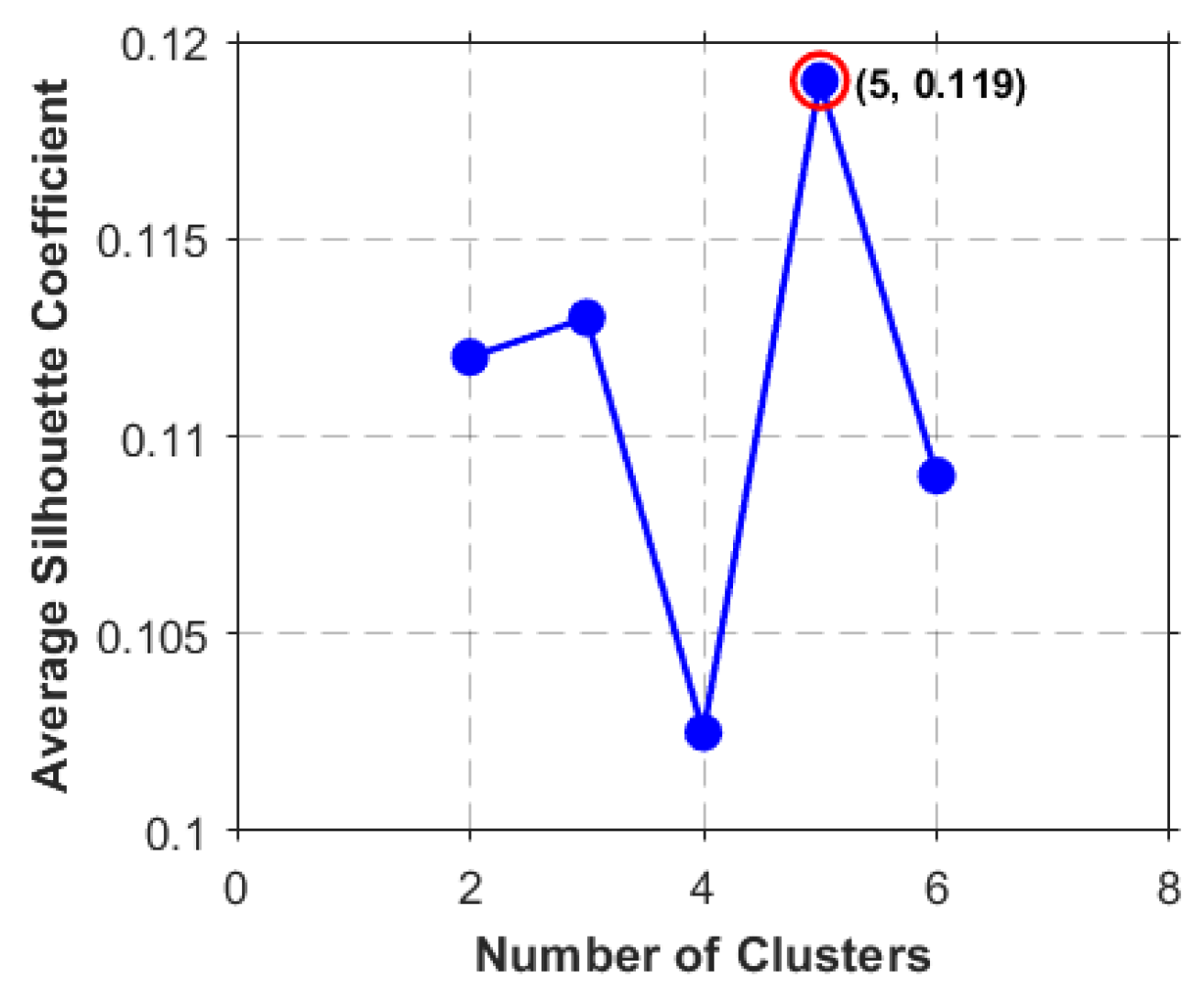
The k-means algorithm is generally determined by the average contour coefficient of the clustering effect. The contour coefficient is greater than zero meaning that the clustering effect is still good [13], as shown by the average contour coefficient of the number of clusters obtained in Figure 4. We took the average contour coefficient of the largest number of clusters, 5, for clustering.

The k-means algorithm’s objective function minimizes the within-cluster sum of squares:

$$J={\sum }_{k=1}^K{\sum }_{x_i\in C_k}{‖x_i-{\mu }_k‖}^2,$$

(16)

The Euclidean distance is defined as

$$d\left(x_i,x_j\right)=\sqrt{{\sum }_{d=1}^D{\left(x_{i,d}-x_{j,d}\right)}^2},$$

(17)

where μ_k is the center of the kth class.

4. Results

4.1. Hierarchical Clustering

In extracting the clustered scenario results, we designated the variable value with the highest frequency of cases as the representative outcome. In this case, there may be bias due to uneven distribution of incident data, which is reflected in the fact that there are studies that take the parameter with the largest percentage of scenarios of a class [18], or the parameter value with the highest number of occurrences of a variable in a class [19].

In this paper, instead of considering only the overall percentage, after eliminating variable values with a small number of cases (which are small and not representative), the relative percentage is obtained by taking the ratio of the number of instances of that variable value in each category to the total number of cases of that variable value to minimize the bias due to the uneven distribution of the data (some variable values with a higher number are still masked by the variable value with the highest number, but its relative percentage is much higher than that of another variable value). Some of the relative percentages of the variable values and the selection of the variable values are shown in

Table 7. Clustering parameter selection is part of the frequency table.

Parameter	Parameter Value	I	II	III	IV	V
Precipitation condition	No	5.7%	62.7%	6.8%	9.7%	3.6%
Visibility	No fog	5.1%	57.2%	6.2%	9.5%	3.1%
Road surface	Good	5.1%	60.4%	6.9%	10.1%	0.0%
A vehicle type	Car	6.0%	67.6%	7.2%	0.0%	4.1%
	Truck	0.0%	0.0%	0.0%	66.7%	0.0%
Time of day	Daytime	4.9%	55.2%	8.4%	8.7%	4.2%
	Evening	6.2%	61.1%	1.2%	9.3%	2.5%
B vehicle type	Car	6.9%	48.6%	8.1%	13.8%	2.4%
	Truck	0.7%	74.7%	1.4%	0.0%	5.5%
Street light status	No street light	1.4%	60.1%	5.5%	13.8%	6.4%
	On	9.8%	52.0%	4.9%	6.9%	0.0%
	Off	6.9%	55.5%	7.5%	5.2%	1.7%
B steering type	No steering	2.2%	67.4%	0.9%	13.2%	2.5%
	Right turn	12.7%	36.7%	21.5%	1.3%	5.1%
	Left turn	10.6%	31.8%	13.6%	0.0%	7.6%
A steering type	No steering	3.8%	68.7%	0.3%	8.6%	3.1%
	Right turn	5.1%	44.9%	6.4%	11.5%	7.7%
	Left turn	8.4%	32.6%	23.2%	11.6%	1.1%
Number of lanes in the direction of travel	1	0.0%	45.8%	19.2%	5.8%	1.7%
	2	12.3%	48.8%	2.5%	11.8%	7.4%
	3	0.0%	79.0%	0.0%	10.1%	0.0%
On-site road environment	Straight	0.0%	63.0%	3.5%	13.5%	7.4%
	General intersection	24.2%	37.4%	6.1%	1.0%	0.0%
	Cross intersection	0.0%	63.6%	12.7%	5.9%	0.0%

.

Specifically, after excluding sparsely represented values, Table 7 presents the decision basis we used to screen and identify the core features (scenario parameters) for the five clustered scenarios (Scenarios I–V). Rather than choosing a value simply because it is most frequent in the overall sample—which can be misleading—we evaluate how concentrated each value is within the scenario categories. For each parameter value v, we therefore compute a “relative percentage,” defined as the proportion of all crashes with value v that fall into scenario k. For example, although car cases greatly outnumber truck cases as vehicle B in the full database, Table 7 shows that, among crashes where vehicle B is a truck, 74.7% occur in Scenario II, whereas among crashes where vehicle B is a car, only 48.6% fall into Scenario II. This indicates that, despite their lower total count, trucks are more strongly associated with Scenario II and thus serve as a more salient defining feature of that scenario than cars.

4.2. Clustering Results

The clustering results obtained from the two clustering methods are shown in

Table 8. Clustering results.

Parameter	Hierarchical Clustering					k-Means Clustering
	I	II	III	IV	V	I	II	III	IV	V
A vehicle type	Car	Car	Car	Truck	Car	Car	Car	Car	Car	Car
B vehicle type	Car	Truck	Car	Car	Truck	Car	Car	Car	Car	Car
On-site road environment	Intersection	Intersection	Crossroads	Straight	Straight	Crossroads	Straight	Straight	Straight	Intersection
Lighting conditions	Street light at night	No street light at night	Daytime	No street light at night	Daytime	Street light at night	Street light at night	Daytime	Daytime	Daytime
Precipitation	No	None	None	None	No	None	None	None	None	None
Road surface	Good	Good	Good	Good	Good	Good	Good	Good	Good	Good
Number of lanes in the direction of travel	2	3	1	2	2	1	2	2	2	2
Visibility	No fog	No fog	No fog	No Fog	Fogless	Fogless	Fogless	Fogless	Fogless	Fogless
A steering type	Left	No steering	Left	Left	Right	No steering	No steering	No steering	No steering	No steering
B steering type	Right	No steering	Right	No steering	Left	No steering	No steering	No steering	No steering	No steering

, which does not show the scenarios with a low number of cases in hierarchical clustering (not representative). Comparing the two sets of clustering results, the scenarios obtained from hierarchical clustering are more obviously differentiated compared to the k-means method, which is caused by the fact that the clustering center of the k-means inevitably tilts towards the dimension with a high number of cases of variable values. As for k-means clustering, it only needs to be interpreted according to the resulting clustering center.

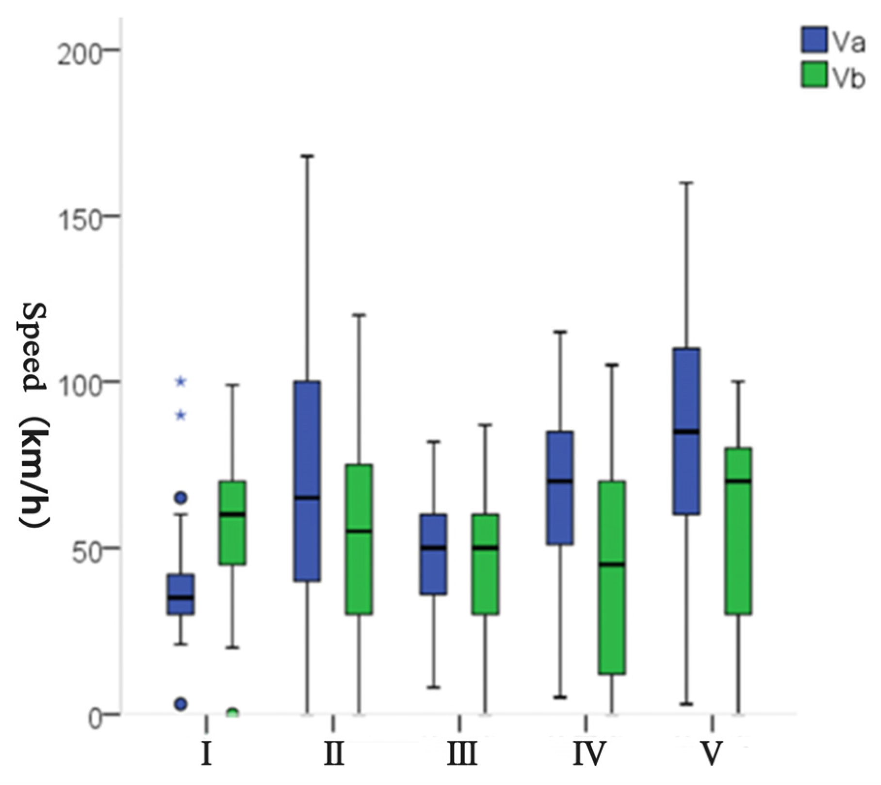
Therefore, the hierarchical clustering results were chosen to extract typical accident scenarios [20], with the upper and lower quartiles of the A and B speeds corresponding to each of these five categories as upper and lower limits, see Figure 5, and the speed intervals are detailed in

Table 9. Hierarchical clustering information (the 95% confidence interval was obtained using the Wilson interval (z = 1.96); there may be slight rounding errors).

Parameter	I	II	III	IV	V
Speed of A (km/h)	30–42	40–100	36–60	51–85	60–110
Speed of B (km/h)	45–70	30–75	30–60	12–70	30–80
Percentage	5%	57%	6%	9%	4%
Injury rate for this scenario	28%	52.9%	30%	10.9%	41.2%
Scenario-level injury rates (Wilson 95% CIs)	14.3–47.6%	47.2–58.8%	16.7–47.9%	5.0–24.0%	21.9–61.3%

. The final five typical scenarios extracted via hierarchical clustering are detailed in Table 9. To provide further statistical validation, the 95% confidence intervals for the mean speed in each scenario have also been calculated and included, offering a more precise estimation of the speed characteristics for each cluster.

We applied the Kruskal–Wallis H test to assess whether medians differ across the five independent scenarios:

k = 5, N = 493; n = (276, 44, 35, 25, 20). All 493 initial speeds of vehicle A are pooled and ranked from smallest to largest (averaging ties); the ranks were reassigned to their scenarios, and each scenario’s rank sum R_i was computed (R ≈ (69,000, 13,000, 7000, 5000, 8000))

“k” represents the number of groups or categories to be compared, “N” is the total sample size, and “n” represents the sample size of each group. (The remaining 93 cases were distributed among smaller, less significant clusters that were excluded from detailed discussion for reasons of statistical reliability.)

$$H=\left[{\displaystyle \frac{12}{N\left(N+1\right)}}{\sum }_{i=1}^k{\displaystyle \frac{R_i^2}{n_i}}\right]-3\left(N+1\right),$$

(18)

in which “k” represents the number of groups or categories to be compared, “N” is the total sample size, and “n” represents the sample size of each group.

Degrees of freedom [21]:

$$df=k-1=5-1=4,$$

(19)

Find the p-value: We compared the H statistic (36.85) and degrees of freedom (4) with the chi-square distribution to calculate the p-value [22]. The Kruskal–Wallis procedure is widely used in road-safety analytics to detect group differences in non-normal indicators (e.g., built-environment contrasts between high- and low-accident areas) [23].

Final p-value: p ≈ 0.000000198

We also report the nonparametric effect size (epsilon-squared) for the Kruskal–Wallis procedure [24]:

$${\eta }_H^2={\displaystyle \frac{H-(k-1)}{N-1}},$$

(20)

Substituting our values yielded a result of approximately 0.067 (small to moderate effect).

Since the calculated p-value was far smaller than our predefined significance level of 0.05, we rejected the null hypothesis, confirming that the characteristics of the accident scenarios did indeed have a significant impact on vehicle speed.

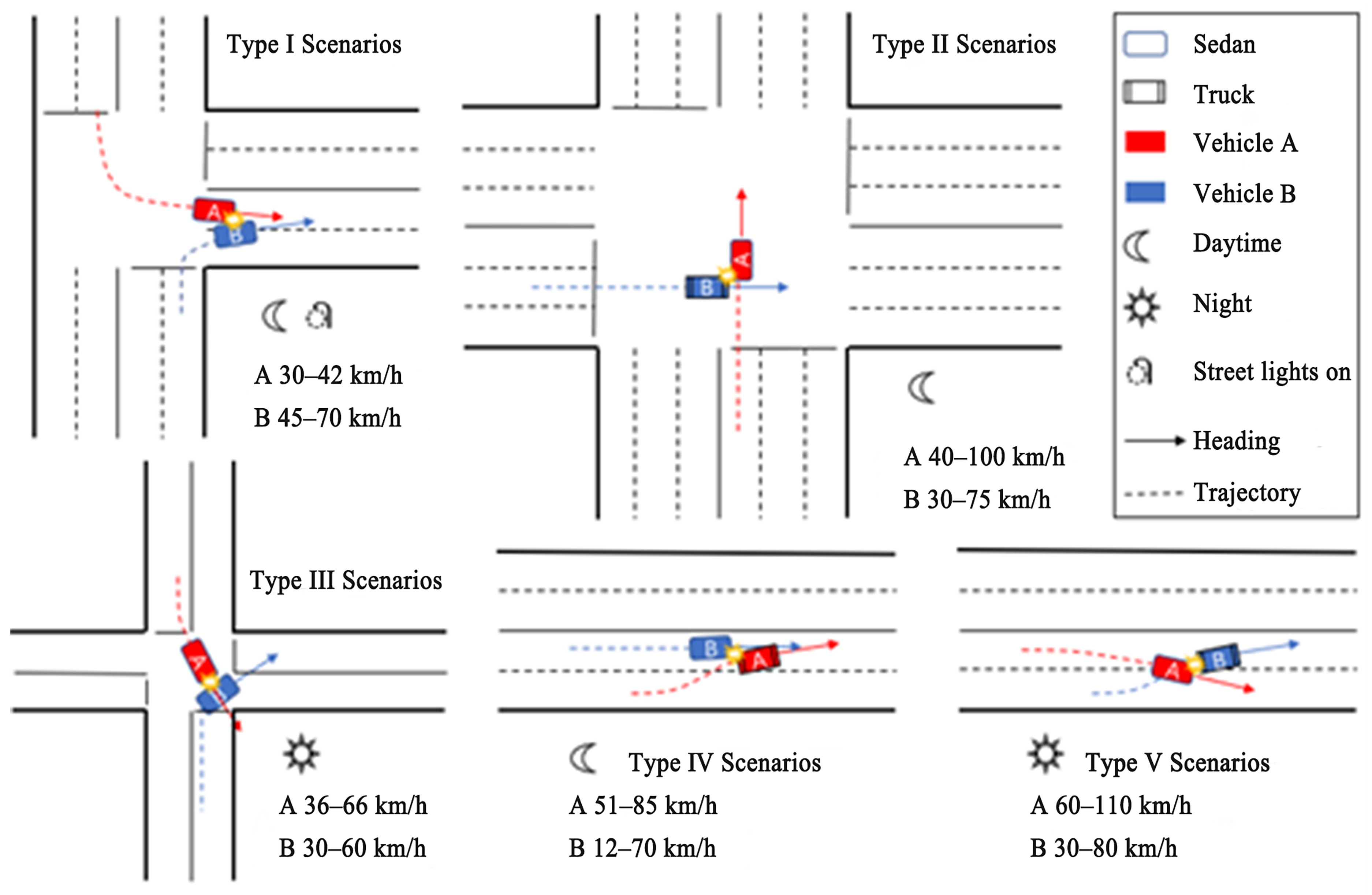
Scenario Type I is an accident between two cars at night in a two-way four-lane intersection with street lights; when car A turns left and car B turns right, the speed interval of car A is 30–42 km/h, and the speed interval of car B is 45–70 km/h.

Scenario Type II is an accident between cars and trucks at night in the absence of street lights in a two-way six-lane intersection. Neither A nor B are steering; the A car’s speed range is 40–100 km/h, and the B car’s speed range is 30–75 km/h. This is the most accounted for scenario in our class of scenarios.

Scenario Type III is an accident between two cars during the daytime at an intersection with two lanes in both directions; when car A turns left and car B turns right, the speed range of car A is 36–60 km/h and the speed range of car B is 30–60 km/h.

Scenario Type IV occurs between trucks and cars at night on a two-way, four-lane straight road without street lights and involves accidents where car A is making a left turn and car B is traveling straight. Car A’s speed range is 51–85 km/h, and car B’s speed range is 12–70 km/h.

Scenario Type V is an accident between a car and a truck during the daytime on a level road with four lanes in both directions; at the time when car A turns right and car B turns left, the speed range of car A is 60–110 km/h, and the speed range of car B is 30–80 km/h.

These five typical scenarios have no precipitation, good road conditions, and good visibility. The scenarios are illustrated in Figure 6. Note that Figure 6 only gives a schematic of the scenarios, and specifics such as collision location and collision angle need to be determined by further research.

Although these diagrams are simplified illustrations, they are based on clustering results derived from actual accident data. Additionally, during the diagramming process, principles for scenario design outlined in domestic and international traffic safety regulations and policy documents were referenced to ensure that the scenarios are realistic, representative, and practical. These diagrams can provide a useful reference for subsequent simulation and modeling, accident research, and autonomous vehicle testing.

5. Discussion

5.1. Scenario-Level Interpretation

Building on the cluster definitions in Section 4, Table 9 reports the share of cases and injury rates by scenario. The percentage of the total number of cases in each scenario category and the percentage of injuries in each scenario are expressed in Table 9. Because the number of cases in other categories is very low (around 1% each), clustering does not categorize the different values of the same variable well; for example, it may cluster a variable within a category to the same single value [25].

In Type IV and Type V scenarios, due to the low traffic volume and the single flat road environment, and considering A vehicle type, lighting conditions have little effect on the speed of vehicles on that flat road. However, the injury ratio in the fourth category is 1/4 that of the fifth category, so lighting condition is an impactful variable for accidents on straight roads.

Type I and Type III scenarios both feature left turns at intersections. Type I includes a four-lane roadway in both directions, hence the roadway width is larger than in Type III, but the upper and lower speed limits of its A vehicles are smaller than those of Type III, indicating that lighting conditions at intersections can influence vehicle speeds.

Type II and Type III scenarios both occur at intersections. The speed of vehicle A is greater at night without street lights than during the day (the traffic flow at the scenario at the time of the accident is less traffic, see Section 2.2), indicating that the number of lanes in the direction of travel and the steering condition of the vehicle have a large impact on the speed of the vehicle at the intersection.

Meanwhile, in Type II and Type III scenarios, lighting, the number of lanes, B vehicle type, and A vehicle speed jointly affect the injury of main vehicle occupants, resulting in a higher injury rate in the latter scenario.

5.2. Weather Effects

The number of cases corresponding to each occupant injury level (minor injuries and above) for each weather condition is shown in

Table 10. The degree of injury corresponding to each weather condition.

Parameter	Slight Injury	≥Serious Injury	Total Number of Injuries	Percentage of Serious Injuries	Percentage of Injuries
No	116	73	442	16.5%	42.7%
Rain	13	10	41	24.4%	56.1%
Snow	3	1	10	10%	40.0%

.

As far as serious injuries are concerned, the frequency of serious injuries to vehicle occupants in accidents occurring when it rained is 7.9% higher than the frequency when it did not rain. The frequency of injuries when it rained is 13.4% higher than when it did not rain, which suggests that rainfall had a greater impact on occupant injuries compared to snowfall. It is noteworthy that the injury frequencies of accidents when it snowed were all lower than those without rain, i.e., extreme weather made drivers drive more cautiously.

5.3. Cross-Method Triangulation and Method Sensitivity

Whereas an effect of precipitation was not reflected by the clustering results due to the low number of precipitation cases, which masked this effect even when relative percentages were taken, the significance obtained from the factor analysis keenly identifies the effect of precipitation on occupant injuries.

We can summarize the following points:

(1)

The most significant factors obtained by all three methods, ANN, DT, and RF, were vehicle parameters, where B vehicle type had a greater impact on occupant injury than A vehicle type.

(2)

From an analysis of the clustering results, it can be concluded that lighting, the number of lanes, B vehicle type, the speed of vehicle A, and precipitation have a greater effect on occupant injury.

(3)

The significance of the variables obtained from the factor analysis showed that the first common factor, consisting of accident pattern, on-site road environment, road classification, and A vehicle speed, had the greatest impact.

(4)

The factor analysis method is more sensitive to small samples in the data than other machine learning methods.

This discrepancy indicates that layered scenario definitions should be used in future work so that rare but safety-critical environmental layers (e.g., precipitation) are preserved in the scenario taxonomy rather than diluted by dominant background conditions.

5.4. Scope and Transferability Beyond Two-Vehicle Interactions

To clarify scope and transferability, we contrast two-vehicle cases with multi-vehicle, VRU-involved, and single-vehicle crashes. Multi-vehicle settings (≥3 actors) introduce additional interaction pathways—such as concurrent or cascading conflicts and potential sensor occlusions—that typically require multi-target tracking and conflict prioritization beyond two-vehicle interactions. VRU scenarios differ from car-to-car settings in target observability and motion variability, which may lead to distinct conflict geometries and testing emphases (e.g., pedestrian/cyclist AEB). Single-vehicle crashes are often dominated by roadway-departure or fixed-object mechanisms. They are more closely addressed by lateral control functions (e.g., LKA/LDW) rather than longitudinal car-to-car mitigation. We therefore position our findings as a baseline for two-vehicle interactions. Extending the framework to multi-vehicle and VRU settings will require explicit modeling of occlusion, cascade effects, and behavioral heterogeneity. Our team is currently developing three-vehicle scenarios and visibility features within the same pipeline; results will be reported separately.

5.5. Limitations

This study has several limitations at the data level that should be acknowledged. First, the sample size is limited. The dataset consists of 493 two-vehicle accident cases from 2011 to 2022. However, the focus on a specific accident type, combined with rigorous data cleaning to handle missing or “unknown/not applicable” entries, reduced the effective number of samples available for modeling. This may affect the stability of the categorical distributions and the statistical power of the analysis.

Beyond the overall sample size, the dataset’s representativeness is also an issue. The CIDAS database exhibits a notable geographic bias; for example, nearly 70% of its cases originated from a single city. This concentration implies that the “typical scenarios” identified in our research may more closely reflect regional characteristics rather than a comprehensive national average. Furthermore, the data is imbalanced regarding environmental conditions, with nearly 90% of accidents occurring in non-rainy weather. This makes it difficult for the analysis to represent high-risk scenarios under adverse weather adequately.

Finally, this study has limitations related to its methodological choices and data availability. First, in the factor analysis stage, a lower eigenvalue threshold of 0.5 was adopted for exploratory purposes to retain more variance (a cumulative explained variance of 87.7%). However, this inevitably led to the inclusion of weaker factors (e.g., visibility), which may have introduced noise into the subsequent cluster analysis.

Second, a more systemic limitation stems from the imbalanced data distribution. Several dominant variable values (e.g., “Good road surface” at 88% and “No fog” at 98.6%) had a disproportionate impact on the distance calculations within the clustering algorithm. This resulted in the five final clustered scenarios exhibiting a high degree of homogeneity in environmental and road conditions (e.g., all scenarios featured no rain, no fog, and good road surfaces). While this reflects the common context in which accidents occur, it may have obscured specific accident patterns that emerge under non-ideal conditions, such as on wet or damaged road surfaces or during periods of limited visibility.

Furthermore, extensive evidence indicates that the vast majority of crashes are attributable to driver-related human errors; recent work estimates that over 90% of road crashes stem from behaviors such as speeding, distraction, fatigue, and failures to yield [26]. However, our dataset lacks key driver-level variables—such as age, physiological state (e.g., fatigue, distraction), and reaction time—constraining the depth of our analysis of accident mechanisms. Consequently, while our models based on vehicle and environmental parameters delineate the contexts in which two-vehicle accidents occur, they cannot fully capture the underlying causes, which are intrinsically linked to driver behavior.

To address these limitations, future research could proceed in the following directions:

Data Balancing: Before modeling, techniques such as oversampling the minority class samples (e.g., cases involving rain/snow or poor road conditions) or undersampling the majority class samples can be applied to balance the class distribution.

Case Weighting: A weighting mechanism can be introduced into the clustering algorithm. Weights can be assigned to samples based on the rarity of their features. For instance, an accident case that occurred in “rainy conditions with potholes” would receive a much higher weight than a case from “clear weather on a good road surface.” This approach would increase the algorithm’s sensitivity to rare but critical events, thereby enabling the discovery of more challenging hazard scenarios that are currently obscured.

Integration of Human Factors Data: Future work should aim to integrate official accident databases with data from Naturalistic Driving Studies (NDS) or driving simulators. This would enable a more comprehensive understanding of the dynamic interactions within the ‘human-vehicle-environment’ system during an accident.

These will be key priorities for our subsequent work. These limitations collectively indicate that future research should integrate more diverse, balanced data that includes crucial human factors to construct a more generalizable test scenario repository.

5.6. Layered Scenario Definition and Future Work

To prevent low-frequency but high-risk scenarios (such as precipitation, low visibility, and road damage) from being diluted by high-frequency background conditions, a layered scenario definition can be employed: A baseline scenario is first formed at the structural layer (road type, intersection configuration, number of lanes, and turning pattern). This is then refined by overlaying the traffic layer (traffic flow, priority relationships), the environmental layer (precipitation, visibility, and road conditions), and the behavioral layer (driver attention and fatigue). The modeling phase combines stratified sampling with sample/feature weighting to ensure that the key, rare conditions at each layer are sufficiently represented in the cluster or scenario library, thus covering both “normal” and “undesirable” scenarios.

6. Conclusions

This study investigated the key factors affecting occupant injury severity in two-vehicle collisions using CIDAS accident data. The analysis revealed that the type of striking vehicle and the collision speed of the host vehicle were the most influential factors contributing to injury outcomes. Environmental variables, such as lighting conditions and precipitation, also played a non-negligible role.

Through factor analysis and clustering, five representative accident scenarios were identified, each reflecting a unique combination of roadway and environmental features. These scenarios offer valuable references for the development of automated driving test protocols and safety evaluation frameworks.

While this research provides useful insights, its focus on two-vehicle accidents suggests that future work should consider multi-vehicle crashes, vulnerable road users, and driver behavior data to improve model generalizability and practical applicability.

References

1. Zhang, X.; Khan, M. Principles of Intelligent Automobiles; Springer: Singapore, 2019. [Google Scholar]
2. World Health Organization. Global Status Report on Road Safety 2018; World Health Organization: Geneva, Switzerland, 2019. [Google Scholar]
3. Zhou, H.; Li, X.; He, X.; Li, P.; Xiao, L.; Zhang, D. Research on safety of the intended functionality of automobile AEB Perception System in Typical Dangerous Scenarios of Two-Wheelers. Accid. Anal. Prev. 2022, 173, 106709. [Google Scholar] [CrossRef] [PubMed]
4. Sujayanont, P.; Muttitanon, W.; Chemin, Y.; Som-Ard, J.; Tippayanate, N. Multiple logistic regression model for assessing the risk factors of traffic accidents: Khon kaen model. In Digital Health and Informatics Innovations for Sustainable Health Care Systems; IOS Press: Amsterdam, The Netherlands, 2024; pp. 1589–1593. [Google Scholar]
5. Wahab, L.; Jiang, H. Severity prediction of motorcycle crashes with machine learning methods. Int. J. Crashworthiness 2020, 25, 485–492. [Google Scholar] [CrossRef]
6. Wu, Q.; Song, D.; Wang, C.; Chen, F.; Cheng, J.; Easa, S.M.; Yang, Y.; Yang, W. Analysis of Injury Severity of Drivers Involved Different Types of Two-Vehicle Crashes Using Random-Parameters Logit Models with Heterogeneity in Means and Variances. J. Adv. Transp. 2023, 2023, 3399631. [Google Scholar] [CrossRef]
7. Ijaz, M.; Lan, L.; Zahid, M.; Jamal, A. A Comparative Study of Machine Learning Classifiers for Injury Severity Prediction of Crashes Involving Three-Wheeled Motorized Rickshaw. Accid. Anal. Prev. 2021, 154, 106094. [Google Scholar] [CrossRef] [PubMed]
8. Ma, J.; Cao, Q.; Ren, G.; Yang, Y.; Deng, Y.; Li, J. Exploring the heterogeneous effects of riding behaviours and road conditions on delivery rider severities in scooter-style electric bicycle crashes involving vehicles. Int. J. Inj. Control Saf. Promot. 2024, 31, 165–180. [Google Scholar] [CrossRef]
9. Dong, X.; Zhang, Q.; Zhang, D.; Wang, C.; Zhang, T. Research and deduction of car-to-TW vehicle AEB test scenarios based on improved clustering methods. J. Adv. Transp. 2023, 2023, 2708201. [Google Scholar] [CrossRef]
10. Wang, H.; Wang, X.; Peng, Y.; Lou, X.; Lee, J. An investigation of ADAS testing scenarios based on vehicle-to-powered two-wheeler accidents occurring in a county-level district in China. Transp. Saf. Environ. 2024, 6, tdae013. [Google Scholar] [CrossRef]
11. Rao, R.; Cui, C.; Chen, L.; Gao, T.; Shi, Y. Quantitative testing and analysis of non-standard AEB scenarios extracted from corner cases. Appl. Sci. 2024, 14, 173. [Google Scholar] [CrossRef]
12. Zhao, Z.; Jin, X.; Cao, Y.; Wang, J. Data mining application on crash simulation data of occupant restraint system. Expert Syst. Appl. 2010, 37, 5788–5794. [Google Scholar] [CrossRef]
13. Field, A. Discovering Statistics Using IBM SPSS Statistics, 4th ed.; Sage Publications Ltd.: Thousand Oaks, CA, USA, 2013. [Google Scholar]
14. Azhar, A.; Ariff, N.M.; Bakar, M.A.A.; Roslan, A. Classification of driver injury severity for accidents involving heavy vehicles with decision tree and random forest. Sustainability 2022, 14, 4101. [Google Scholar] [CrossRef]
15. Wang, X.; Su, Y.; Zheng, Z.; Xu, L. Prediction and interpretive of motor vehicle traffic crashes severity based on random forest optimized by meta-heuristic algorithm. Heliyon 2024, 10, e35595. [Google Scholar] [CrossRef]
16. Habibzadeh, M.; Hasan Mirabimoghaddam, M.; Sadat Haghighi, S.M.; Ameri, M. Presentation of artificial neural network models based on optimum theories for predicting accident severity on rural roads in Iran. Transp. Res. Interdiscip. Perspect. 2024, 25, 101090. [Google Scholar] [CrossRef]
17. Gu, C.; Xu, J.; Li, S.; Gao, C.; Ma, Y. Injury risk assessment and interpretation for roadway crashes based on pre-crash indicators and machine learning methods. Appl. Sci. 2023, 13, 6983. [Google Scholar] [CrossRef]
18. Song, Y.; Chitturi, M.V.; Noyce, D.A. Automated vehicle crash sequences: Patterns and potential uses in safety testing. Accid. Anal. Prev. 2021, 153, 106017. [Google Scholar] [CrossRef]
19. Nitsche, P.; Thomas, P.; Stuetz, R.; Welsh, R. Pre-crash scenarios at road junctions: A clustering method for car crash data. Accid. Anal. Prev. 2017, 107, 137–151. [Google Scholar] [CrossRef]
20. Esenturk, E.; Wallace, A.; Khastgir, S.; Jennings, P.A. Identification of traffic accident patterns via cluster analysis and test scenario development for autonomous vehicles. IEEE Access 2022, 10, 6660–6675. [Google Scholar] [CrossRef]
21. Gibbons, J.D.; Chakraborti, S. Nonparametric Statistical Inference, 6th ed.; Chapman and Hall/CRC: New York, NY, USA, 2020. [Google Scholar]
22. Perticone, A.; Barbani, D.; Baldanzini, N. An enhanced method for evaluating the effectiveness of protective devices for road safety application. Accid. Anal. Prev. 2024, 203, 107615. [Google Scholar] [CrossRef]
23. Yan, R.; Hu, L.; Li, J.; Lin, N. Accident severity analysis of traffic accident hot spot areas in Changsha city considering built environment. Sustainability 2024, 16, 3054. [Google Scholar] [CrossRef]
24. Ben-Shachar, M.S.; Lüdecke, D.; Makowski, D. Effectsize: Estimation of effect size indices and standardized parameters. J. Open Source Softw. 2020, 5, 2815. [Google Scholar] [CrossRef]
25. Sander, U.; Lubbe, N. The potential of clustering methods to define intersection test scenarios: Assessing real-life performance of AEB. Accid. Anal. Prev. 2018, 113, 1–11. [Google Scholar] [CrossRef]
26. Zhao, W.; Gong, S.; Zhao, D.; Liu, F.; Sze, N.N.; Quddus, M.; Huang, H. A spatial-state-based omni-directional collision warning system for intelligent vehicles. IEEE Trans. Intell. Transp. Syst. 2024, 25, 14344–14358. [Google Scholar] [CrossRef]
Figure 1. Data parameters.
Applsci 15 09819 g001
Figure 2. (a) Speed distribution of vehicle A; (b) speed distribution of vehicle B.
Applsci 15 09819 g002
Figure 3. Cluster scree plot.
Applsci 15 09819 g003
Figure 4. Average contour coefficient of k-means.
Applsci 15 09819 g004
Figure 5. Speed ranges of vehicles A and B in each scenario. Circles (o) denote mild outliers (1.5–3 × IQR), and asterisks (*) denote extreme outliers (>3 × IQR).
Applsci 15 09819 g005
Figure 6. Schematic diagram of typical scenarios.
Applsci 15 09819 g006