Abstract
This study is the first to directly compare natural dynamic penumbra shadows with experimentally replicated constant-intensity shadows on photovoltaic modules, providing new insights into the limitations of conventional shadow approximations found in the existing body of knowledge. Neutral density filters were deemed the most appropriate method for replicating a constant-intensity shadow, as they reduce visible light relatively uniformly across the primary silicon wavelength range. Preliminary experiments established the intensity values for each neutral density filter chosen to be able to match with the 29 dynamic penumbra shadows being replicated by both the size of shadow and the averaged intensity. The results revealed that while constant-intensity shadows and dynamic penumbra shadows produced similar overall power loss magnitudes, the constant-intensity shadows consistently led to higher losses, averaging 9.65% more, despite having the same average intensity and shadow size. Regression modelling showed similar curvature trends for both shading types (Adjusted R2 = 0.895 for constant-intensity shadows and Adjusted R2 = 0.743 for dynamic-intensity shadows), but statistical analyses, including the Mann–Whitney U-test (p = 0.00229), confirmed a significant difference between the power loss output for the two penumbra shadow conditions. Consequently, the null hypothesis was rejected, confirming that the simplified constant-intensity shadows represented in the literature cannot accurately replicate the behaviour of dynamic-intensity penumbra on photovoltaic modules.
1. Introduction
Shading in photovoltaic (PV) applications is governed by several mechanisms that influence both the spatial and temporal distribution of light across PV systems. Hard shading, typically caused by large opaque structures such as buildings, results in distinct umbra regions where irradiance is completely obstructed, whereas thin-object shading produces more complex patterns that often include both umbra and penumbra regions with gradual intensity transitions [1,2,3]. The dynamic nature of thin-object shading, such as from poles, overhead cables, or vegetation, introduces irregular and time-dependent fluctuations in incident irradiance. These variations are further compounded by atmospheric conditions, including cloud cover and diffuse irradiance, which modulate shadow intensity and geometry [4,5]. As a result, shading mechanisms cannot be adequately characterised by static or uniform assumptions but rather require a consideration of object geometry, distance from the module, and spectral as well as angular properties of incoming radiation. This understanding is essential for accurately modelling and mitigating shading effects in practical PV deployments.
The implications of shading extend beyond individual PV modules, carrying significant consequences for broader renewable energy applications. In large-scale solar farms and rooftop urban solar systems, shading can induce disproportionate power losses, generate mismatch conditions, and accelerate module degradation through hot-spot formation [6,7]. In microgrids and distributed energy systems, the intermittency introduced by partial shading disrupts voltage stability, complicates energy management, and necessitates the integration of advanced mitigation technologies such as module-level power electronics or adaptive MPPT algorithms [8,9]. Furthermore, urban environments amplify shading challenges due to complex geometries and moving obstructions, requiring simulation tools and design practices that account for dynamic penumbra effects rather than simplified hard-shadow approximations [2,4]. Consequently, shading is not merely a localised phenomenon but a systemic constraint on renewable integration, directly influencing energy yield, system economics, and long-term reliability. Addressing these implications requires both physical experimental modelling of shading mechanisms and targeted design strategies tailored to specific renewable energy applications.
State-of-the-art research on the PV shading effect, such as the research conducted by Ismail et al. [10], Klugmann et al. [11], and Aljumaili et al. [1], primarily emphasises the adverse effects of hard shading caused by umbra shadows, resulting from the complete obstruction of direct sunlight. However, scientifically, a shadow is categorised into two distinct parts, the umbra and the penumbra [12]. The umbra is located directly in line with the object and the light source on the surface, creating the darkest part of the shadow, associated with hard shading on PV sources. Subsequently, surrounding the umbra shadow portion is the penumbra, which extends outward and forms a partially lit region [13]. Moreover, in the realm of photovoltaics (PVs), partial shading has predominantly consisted of partially shading PV modules directly on the solar cell, as seen in the research by the authors of [4,14]. The results of [14] demonstrate that shading 50% of the cell resulted in approximately a 50% power reduction, while shading one-quarter or one-eighth of the cell led to proportionally smaller reductions. Moreover, the shadow being applied is a constant-intensity shadow, replicating a hard shadow, rather than a dynamic-intensity shadow, which more accurately represents the natural shadow formation observed on a PV module under shading conditions, as represented in [3].
Similarly, Ref. [15] demonstrated that shading the first row of monocrystalline solar cells with black opaque paper reduced the PV module’s power output to just 0.48% of its initial value. When the bottom 5 cm and 10 cm of the module, approximately one-third and two-thirds of its area, were shaded, the power output dropped to 77.04% and 37.19%, respectively. Evidently, the power loss results observed above are high. However, in real-world scenarios where penumbra is present, the power loss percentages seen are significantly lower due to the loss in shadow intensity when the shading object is situated far away from the PV source. Particularly, Feng et al. [16] focused on thin linear shading using a vertical 10 m pole placed in close proximity to the PV module, where the initial power loss on the PV module resulted in a 9.21% power loss. Moreover, as the pole was moved further away, the power loss was reduced to between 2% and 5%, exemplifying that, as the distance increases, the penumbra shadow replaces the umbra shadow, resulting in a power loss decrease due to the lighter shadow intensity. In a mathematical model approach, Ref. [3] presented a brightness profile model for umbra and penumbra regions under direct radiation, capturing the overall intensity distribution. The authors further demonstrate that the brightness distribution reflecting the intensity, and the brightness profile of the umbra and penumbra, are the most influential factors in analysing the impact of a thin linear shadow on a PV source. However, the model does not distinctly isolate the specific contribution of the penumbra to the observed power loss. In contrast, Ref. [17] acknowledges the penumbra shadow, in its isolated state, as a condition that provides rise to multiple local maximum power points. This study highlights that this complexity necessitates the use of more advanced algorithms to effectively track the global maximum power point. Having said that, in contrast to the works by the authors of [17,18], where the penumbra shadow is represented by high-quality imagery, the authors do not provide evidence on the type of penumbra shadow being referred to, which in turn, does not provide the reader with the necessary evidence on the type of penumbra being analysed.
2. Research Work and the Shading Process
From the literature reviewed in the preceding section, it is evident that further scientific research should be directly converged towards the penumbra shadow on its own, not merely as a byproduct of partial shading. This observation lies in the findings, which have demonstrated that penumbra shadows become lighter in nature as the shading object moves away from the surface of the PVs, causing a reduction in the power loss impact on PVs. Nonetheless, exclusive penumbra shadows, characterised by a gradual decrease in light intensity, have not been extensively investigated in their isolated state from the umbra shadow. This is due to many studies classifying penumbra as a ‘boundary’ [19] (p. 1237) or of a ‘diffused nature’ [19] (p. 1236), instead of as a detrimental part of a shadow on a PV source. However, the definition of a penumbra shadow has been interpreted in multiple ways by different scholars. Authors such as Murali et al. [20] have depicted the penumbra as having a constant intensity, as seen in Figure 1a. This definition of penumbra is often intended for visual simplification only, as a true penumbra features a gradual transition in intensity towards the non-shaded region, ‘no shadow’, as in Figure 1b. Indeed, Dendrinos [21] has presented a penumbra shadow as having a gradient realistic effect, such as that captured in Figure 1b [22].
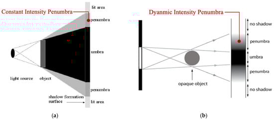
Figure 1.
(a) The principle of shadow formation indicating an umbra and penumbra, where the penumbra is presented as having a uniform grey intensity value, rather than a gradient effect [20]. (b) A representation of an umbra and penumbra shadow, with the penumbra being shown as a dynamic-intensity penumbra shadow [22].
This paper, therefore, aims to investigate whether the gradient characteristics inherent to the penumbra region (as defined by Dendrinos [21] and Ramanath et al. [23]) can be represented instead by simply using a shadow of constant intensity, as interpreted by Muali et al. [20]. It is hypothesised that there is no statistical significance between the power loss of dynamic-intensity penumbra shadows and their constant-intensity counterparts (null hypothesis), whereas the alternative hypothesis posits a statistically significant difference. This will aid in evaluating the scientific validity of the assumption that a penumbra with gradient characteristics, known as a dynamic-intensity penumbra, can be approximated to a single, uniform intensity value. This is mostly applicable to thin-object shading, as demonstrated in previous work in [24,25], which showed substantial complex shadow formation when compared to those found in the literature dealing with hard shading or with the placement of an opaque object on the PV module to mimic shading conditions.
To elucidate the specific shadow characteristics examined in this paper and to clarify the two shadow forms, Figure 2a starts by demonstrating an image of a penumbra-only instance at a substantial distance from the PV source. This shadow instance shall be referred to as a ‘dynamic-intensity penumbra shadow’. In contrast, the corresponding average intensity of the dynamic-intensity penumbra shadow of Figure 2a shall be termed as a ‘constant-intensity shadow’ and is visualised in Figure 2b.

Figure 2.
(a) The formation of a sample dynamic-intensity shadow by a thin sample object. (b) The corresponding constant-intensity shadow, bearing the same overall size and average intensity.
The prior scientific work on thin-object shading, presented in [24,25,26], has so far involved casting shadows directly onto the PV module using thin objects and analysing their relationship and correlation between attributing variables and power loss. In contrast, this paper focuses on replicating penumbra-only shadow instances, similar to that shown in Figure 2a, using a controlled method to achieve a constant-intensity shadow. This approach replicates the dynamic-intensity property while preserving the key shadow characteristics of shadow size and light attenuation. To clarify, shadows such as those in Figure 2a depicting a dynamic-intensity penumbra-only shadow, will not use thin objects as a subject to create the shadow but shall opt for alternative materials capable of attenuating light until the final shadow is comparable to that in Figure 2b. The justification of the material used will be outlined in Section 3.1. The goal is to evaluate how well these constant-intensity shadows, created using alternative light-attenuating materials rather than physical thin objects, can replicate the PV performance of dynamic-intensity penumbra shading.
3. Materials and Methods
This section outlines the materials and methods chosen specifically to replicate the dynamic-intensity penumbra-only shadow. Section 3.1 focuses on the appropriate material selection, which was chosen based on an analysis of several options outlined. This is followed by a comprehensive description of the setup conditions in Section 3.2. Moreover, Section 3.3 quantifies the intensity associated with each of the chosen material grades, while Section 3.4 presents the method used to directly compare the dynamic-intensity penumbra with the constant-intensity shadow.
3.1. Choosing the Appropriate Material to Replicate a Dynamic-Intensity Penumbra-Only Shadow
A penumbra is formed when an opaque object partially blocks light from an extended source [27]. Unlike the umbra, which represents total shadow, the penumbra is a region of partial shadow. This effect cannot be produced using a point light source, as that would result only in an umbra. Moreover, since the penumbra shadow gradually transitions from dark to light intensity, the material chosen to replicate the penumbra must be translucent to allow partial light transmission and form a non-black shadow. Moreover, since Gabrijelčič et al. [28] denote a shadow as the absence of light, the material chosen must also be able to reduce the light in a relatively constant manner, according to the intensity of the shadow. This should be completed, in particular, throughout the wavelengths of the monocrystalline Si bandgap, since this study will analyse the effect on a PV source.
Various translucent materials have been explored for their light transmission, although not necessarily directly in the field of PVs. Serrano et al. [29] denote that traditional substrates such as clear glass offer high visible light transmittance. However, clear glass falls short in reducing light systematically without any additional coatings due to its limited diffusive capacity and poor control over spectral filtering in its raw state. Moreover, Duarte [30] found that clear glass transmitted 74.3% of the source lighting, while tinted and laminated glass can significantly reduce UV radiation. For example, green glass was found to fully block Ultraviolet A (UVA) wavelengths, whilst blue-tinted glass may transmit only 56.8% of the source lighting [30]. However, the amount of light transmittance through glass all depends on the material and composite chosen, introducing spectral mismatch, especially when applying tinted layers. In addition to glass material, Spitz et al. [31] also mention acrylic polymers, particularly the UV-transmitting (UVT) type, as a potential translucent material of choice. However, these types of materials have the tendency to suffer degradation in UV transmittance upon prolonged exposure to sunlight, with measurable losses occurring after only several hours, making them suitable as a material to constantly reduce light across the wavelengths required.
According to Simonot et al. [32], accurately characterising the optical and visual properties of translucent materials as a function of their shape and thickness remains a significant challenge in scientific research, owing to the difficulty in maintaining a consistent spectral distribution of the transmitted light. One sector that relies extensively on translucent materials and has achieved a high level of engineering precision in controlling light transmittance is photography, in particular, the use of photographic filters, engineered for controlled light modulation. Furthermore, the calibrated nature of photographic filters provides the precision and reputability required for scientific use.
Among the various photographic translucent filters available, Kalyani [33] describes absorption filters as compounds that consume certain wavelengths of light and transmit others. Thus, they were deemed unsuitable for replicating the penumbra-only shadow transposed on the PV module. This is due to such filters altering the spectral composition by absorbing only specific wavelengths [33]. In the context of this article, the focus is specifically on penumbra-only shadows, which, by nature, uniformly attenuate light across all wavelengths due to the partial obstruction of the light source. Given that a shadow represents a reduction in overall light rather than selective wavelength absorption, absorption filters were deemed unsuitable for this study. Likewise, colour compensating and balancing filters, which are designed to adjust RGB colour balance and colour temperature, were not considered appropriate. This is because their primary function is to modify spectral composition rather than reduce light intensity uniformly without introducing chromatic shifts [34].
Optical-grade glass filters and coated polymer filters, such as neutral density (ND) and graduated ND filters, offer standardised and calibrated attenuation across a vast spectrum of light, specifically focusing on visible light (380–700 nm). Heron et al. [35] defined ND filters as being capable of reducing the intensity of light without changing the colour composition of the original object. These filters are manufactured to strict tolerances, ensuring spectral neutrality and stability over time. Their ability to produce consistent, predictable light transmittance makes them superior to other preceding translucent materials outlined in this section.
Two main types of ND filters are commercially available: constant transmittance filters, which uniformly reduce light across their entire surface (as illustrated in Figure 3a), and graduated ND filters, shown in Figure 3b. Graduated ND filters feature a transition in light intensity, ranging from full density (black, pixel value 0) to no density (white, pixel value 255), typically positioned at the upper and lower portions of the filter. This gradient closely resembles the dynamic-intensity profile of a penumbra shadow. Even though the graduated ND filters are suitable to mimic penumbra shadow, the aim of this article is to determine whether the average constant intensity of the penumbra shadow can be utilised to simplify the dynamic-intensity penumbra shadow. Therefore, instead of opting for graduated ND filters, ND filters having a single constant intensity were deemed more suitable for the investigation conducted in this article.
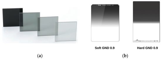
Figure 3.
(a) A constant transmittance light ND filter [36]. (b) An ND filter representing a graduated light transmittance [37].
In a 2024 review published by Willey [38], only eight scientific publications were identified as specifically focused on the development of ND filters. In his concluding remarks, Willey affirmed that ND filters exhibit consistent wavelength-independent attenuation, particularly between the 400 and 1000 nm range. This spectral range closely aligns with the effective response window of crystalline silicon PV cells, which spans approximately 300 to 1100 nm [39]. Consequently, ND filters were identified as suitable candidates for uniformly reducing light intensity without heavily altering the spectral distribution of light, primarily within the visible spectrum [40]. For this reason, they were considered the most appropriate option for replicating dynamic-intensity penumbra shadows (such as penumbra-only formations) using a constant-intensity approach.
Given the novelty of this methodology in the context of shadow replication, preliminary experimentation was necessary to evaluate the suitability and optical behaviour of ND filters for this purpose, particularly considering the limited literature on their application in simulating penumbra shading. The setup conditions as well as the PV sources used for the forthcoming experimentations will be subsequently presented in Section 3.2.
3.2. Setup Conditions and PV Sources Utilised
The forthcoming experimentations were conducted at the premises of the ISE on 4 July 2024, under clear sky conditions, and without external shading from nearby structures. An on-site weather station equipped with a pyranometer continuously recorded global irradiance, including both direct beam and diffuse components, at 10 min intervals throughout the testing period. The irradiance data were used to correct the power output to STC, following the method outlined in Procedure 1 of IEC 60891:2021, which employs current and voltage correction equations [41]. Power loss measurements were recorded using a DATAQ DI-808 data logger, with dedicated inputs for both the control and shaded PV modules, similar to the methodology in Refs. [24,25].
Both modules were mounted horizontally at a 0° inclination to minimise ground reflected radiation (albedo), thereby reducing its influence on incident light intensity. The experimental procedure for comparing power loss followed the guidelines in Section 4.1 of IEC 60904-1:2020 [42] and was further supported by the fixed load-point measurement methodology detailed in prior work outlined in Ref. [26].
To assess differences in power output performance and thereby determine the power loss metric, two identical PV modules were required: one serving as the control and the other as the experimental shaded module, following the methodology established in [24,25]. Ideally, the same small-scale PV modules, with no bypass diodes, bearing dimensions 299 mm × 662 mm, as those used in Ref. [25] would have been employed throughout this article to maintain experimental consistency. However, despite their small size, the overall dimensions of those PV modules exceeded the size of the ND filter sheets provided by the manufacturer (533 mm × 610 mm).
Consequently, two smaller PV modules, bearing overall dimensions of 235 mm × 335 mm, were sourced, with their electrical characteristics detailed in Table 1. These modules were used exclusively in the preliminary experiment presented in Section 4.1.1, which aimed to investigate the impact of varying the vertical elevation of ND filters above the PV surface. To ensure consistency between the control and experimental shaded modules, both of which exhibited near-identical electrical specifications and dimensions, a calibration correction factor was applied. The calibration process resulted in the chosen PV module acting as the shaded PV. The latter was found to generate 0.26% more power than the control PV module under unshaded conditions. This difference was calculated by averaging 15 min of 1 s interval power data under full illumination. Moreover, to obtain a baseline initial power output for both the PV modules, the power readings of the control PV module were increased by 0.26% to align with the baseline output of the shaded PV module under identical test conditions.

Table 1.
The electrical characteristics of the PV module used for the preliminary experimentation.
3.3. Quantifying the Intensity Associated with Each ND Filter
Due to the novelty of the proposed methodology, preliminary experimentation was necessary to verify the suitability of ND filters as a material capable of attenuating gradient light in order to produce a constant-intensity ND filter shadow. For this purpose, flexible gelatine-based ND filter sheets were sourced from Lee Filters, a subsidiary of the Panavision Group and one of the leading manufacturers of optical filters in the United Kingdom, specialising in optical technology.
The ability of ND filters to reduce visible light is quantified by their optical density (OD), a logarithmic metric that indicates the extent to which light is blocked. For example, an OD value of 0.3 corresponds to approximately 50% light transmission and is typically denoted following the acronym ‘ND’. However, for clarity and ease of interpretation in this study, OD values are instead expressed as the percentage of light transmittance reduction (TR), representing the proportion of light blocked, as illustrated in Equation (1).
The first ND filter selected was the lowest TR level commercially available non-opaque option, designed to attenuate sunlight by approximately 95% (ND 1.2), as shown in Figure 4. Additionally, Edmund Optics, a globally recognised manufacturer of optical components, provides a theoretical basis for logarithmically increasing light attenuation through the stacking of multiple ND filters, thereby enabling multilayer filtration [43]. However, to date, no peer-reviewed scientific studies have validated the reliability or optical consistency of stacked ND filters. While this concept warrants further investigation, it lies beyond the scope of the present study. As a result, a single-layer ND filter configuration was adopted and maintained throughout the experiments described in this article.
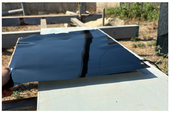
Figure 4.
A single ND filter rated at 95% TR covering the PV module.
One observation that can be inferred from Figure 4 is the lack of space between the ND filter and the PV module. This arises from directly placing the ND filters on top of the PV module, leaving no physical space for capturing images of the constant-intensity shadow and limiting the ability to measure shadow intensity. Therefore, the setup shown in Figure 4 was deemed impractical for image acquisition. To overcome this limitation, a separation distance of 50 cm between the ND filter and the PV module was established, allowing sufficient space to position the camera between the filter and the module for shadow imaging.
To evaluate the impact of this elevation on PV performance, power output differences between the shaded and unshaded modules were measured across varying distances. A range from 10 cm (lower bound) to 50 cm (upper bound) was tested in 10 cm increments, as illustrated in Figure 5a,b. This provided a basis for assessing whether increasing the filter-to-module distance introduced a significant deviation in power output.
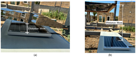
Figure 5.
(a) The ND filter positioned at 10 cm from the PV module. (b) The ND filter repositioned at 50 cm from the PV module to accommodate for image capture.
The 95% TR filter was selected for this evaluation to assess whether variations in filter distance affect the power output of the shaded PV module. This specific grade was chosen due to its dark intensity characteristics, resulting in the highest observed power loss and lowest intensity values, thus representing a worst-case scenario for ND filter application. To ensure repeatability and accuracy, each experimental condition was subject to 50 readings (a measurement every 0.25 s), and the power loss values were averaged into a single value. The results of this preliminary investigation are presented in Section 4.1.1.
To facilitate a comparative analysis across different penumbra conditions, a range of constant-intensity ND filter shadows exhibiting varied pixel intensity values was required. Consequently, in addition to the 95% TR filter, which was previously used to assess the effect of distance on power loss, multiple ND filters with varying TR% grades were additionally sourced. These were required to create a multi-intensity dataset of different constant-intensity shadows, with the aim of subsequently replicating the same intensity level of the chosen dynamic-intensity dataset. This will be discussed more in depth in Section 4.2. Each filter was used to approximate a uniform, constant-intensity shadow. In contrast to naturally occurring dynamic-intensity penumbra shadows described earlier in this section, the shadows produced by the ND filters maintain a constant intensity across the shaded area. The characteristics of each filter and the corresponding intensity values are summarised in Table 2.
Table 2.
The single-layer ND filters used during the experimentation with the converted TR level determined using Equation (1).
The spectral characteristics of each ND filter are presented in Figure 6, based on spectroscopy data provided by the manufacturer. These data are provided to ensure transparency and reproducibility of the methodology. From Figure 6, it was observed that all seven ND filters exhibited consistent attenuation across the visible spectrum, with the exception of a slight increase in transmission between 650 nm and 700 nm. The latter is an identified limitation of this experimental setup.
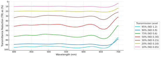
Figure 6.
Spectroscopy data for the ND filters used in this work, as provided by the manufacturer.
In addition to the specified TR levels, it was necessary to determine the intensity values of the constant-intensity ND filter shadows produced by the full range of ND filters to enable a direct comparison with the corresponding dynamic-intensity penumbra shadow instances. This will be detailed in Section 3.4.
In contrast to the preliminary experimentation, where the ND filter cast a shadow directly onto the PV module surface, this second procedure employed a uniform white surface sheet placed over the module. This modification was introduced since the reflective properties and surface texture of the PV module were found to introduce visual distortions that could compromise the reliability of intensity measurements. Therefore, a white surface sheet was used to provide a consistent and controlled imaging background. Failure to capture the image using the white plain surface sheet would result in background pixels being misclassified as shadows, which could potentially produce a false quantification of the shadow intensity being captured. Each ND filter listed in Table 2 was individually positioned at a fixed distance of 50 cm above the PV module surface, and a corresponding image was captured for each case, as illustrated in Figure 7. To maintain uniformity and ensure reproducibility, all images were acquired using the Apple iPhone 15, designed in California and manufactured in Taiwan, with bearing camera settings of ISO 200, a shutter speed of 1/60s, and an aperture of f/1.6. Following the image analysis approach outlined in [44,45], each RGB image was converted into an 8-bit greyscale format using the OpenCV (cv2) library in Python 3.12.0, in accordance with the methodology described in Ref. [46].
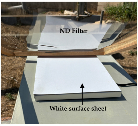
Figure 7.
The image capture setup involving a white surface sheet placed over the PV module, with an ND filter positioned on top.
Unlike a conventional DSLR camera, the iPhone 15’s built-in camera does not allow manual adjustment of ISO or shutter speed by default, and its aperture remains fixed due to hardware constraints. To overcome these limitations, the third-party application Halide v2.17.15 (available on the iOS App Store) was employed. Halide interfaces with Apple’s AVFoundation framework, enabling full manual control of camera settings and thereby allowing replication of the parameters described previously. Using this application, all camera settings were fixed across trials, ensuring consistency and increasing confidence in the accuracy of the image capture. Furthermore, to minimise variability, the iPhone 15 was mounted on a tripod with adjustable height, which ensured a stable and repeatable imaging setup. A white surface sheet, as visualised in Figure 7, was employed as a calibration background to standardise pixel intensity and ensure uniform imaging conditions. This approach minimised variability due to lighting, background texture, and other environmental factors, thereby improving the consistency and reliability of the captured images.
A dataset of pixel intensity values corresponding to the full range of ND filters was compiled, with the results presented in Section 4.1.2. However, as noted by Soni et al. [47], raw pixel values (ranging from 0 to 255) obtained from images captured using portable devices (such as the iPhone 15) do not directly represent actual light intensity due to the non-linear response of the camera sensor. This non-linearity is primarily introduced by gamma correction. The latter is a standard image processing technique applied to align captured luminance data with the human visual system’s sensitivity, particularly enhancing detail in darker regions [47,48].
The iPhone 15 used in this study applies a default gamma correction factor of 2.2 to smooth the transition from black to white on digital displays [19,49]. As a result, it is necessary to invert this gamma correction when processing the intensity values derived from the captured images. This inversion removes the portable devices’ built-in correction and restores the true, real-world intensity values, ensuring accurate scientific measurement of pixel intensity, as emphasised by Carlos et al. [49] and Farid [50]. The conversion from camera-recorded pixel intensity to the real-life intensity is performed using Equation (2), as previously applied by Farid [50]. In this equation, u represents the normalised pixel intensity (ranging from 0 to 1) as recorded by the iPhone 15 camera, and γ is the gamma correction factor, in this case, 2.2 [49]. By applying gamma correction, this study mathematically reverses the perceptual adjustments introduced by the iPhone 15 camera, allowing pixel values to reflect true physical light intensity.
As a result, Section 4.1.2 includes a comparison of gamma-corrected pixel intensities against the raw values, to ensure that the measured intensity more accurately reflects true light attenuation caused by the ND filters.
3.4. Direct Comparable Method Used Between a Dynamic-Intensity Penumbra Shadow and Constant-Intensity Shadow
This section aims to determine whether the null or alternative hypothesis identified in Section 1 should be accepted in response to the research gap identified. To support the comparative experimental analysis between the dynamic-intensity penumbra and the constant-intensity penumbra, Table 3 presents the relevant variables, that is, thickness, distance, and power loss, along with the sources from which their values were derived. The blue rows represent dynamic-intensity penumbra shadow, whereas the red rows symbolise the constant intensity shadow. Each column in the table will be explained in detail in the subsequent discussion. Moreover, Figure 8a presents a visual comparative diagram of the setup representing the penumbra-only dynamic-intensity penumbra shadow instances, while comparably, Figure 8b illustrates the constant-intensity shadow setup using the ND filters.
Table 3.
Comparative value sourcing table between the dynamic-intensity penumbra shadow and the constant-intensity shadow.
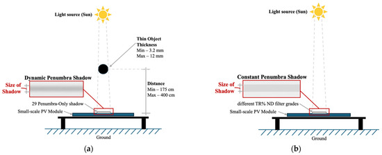
Figure 8.
A visual comparison between (a) the setup used for penumbra-only instances and (b) the setup used for replicating the shadow transposed using the ND filter.
The dynamic-intensity penumbra shadow dataset used in this analysis, corresponding to the experimental setup shown in Figure 8a, was sourced from prior work detailed in [26]. In the latter, 104 instances of thin-object shading were quantified. From these, 29 instances were identified as penumbra-only shadows, based on their light intensity profiles. These instances varied in object thickness, distance from the PV module, and associated percentage power loss, as detailed in the first three columns of Table 3. The remaining 70 cases were excluded from this comparative analysis due to the presence of both umbra and penumbra regions within the shadow formation. The selected 29 penumbra-only instances occurred predominantly at distances between 175 cm and 400 cm, as indicated in Figure 8a. The upper bound of this distance range (400 cm) was set as a constraint, owing to the physical limitation incurred when the projected penumbra shadow exceeded the 100% surface area of the quarter-cut solar cell used in the small-scale PV module. Additionally, the thickness of the thin objects for the chosen 29 penumbra-only instances ranged from ⌀3.2 mm to ⌀12 mm, as illustrated by the examples shown in Figure 8a.
The objective was to preserve the two most critical attributes identified in Ref. [25], shadow size and intensity, for both the dynamic-intensity penumbra shadow (represented in blue in Table 3) and the constant-intensity penumbra shadow (represented in red in Table 3). The fourth and fifth columns of Table 3 present the source data used to replicate the size of the dynamic-intensity penumbra shadows. The shadow sizes for all 29 penumbra-only instances were extracted from the prior work on thin-object shading presented in Ref. [25]. Accordingly, 29 distinct shadow sizes were required to be replicated. To achieve this, ND filter sheets were cut into horizontal strips corresponding to each of the 29 shadow sizes and applied to the surface of the PV module, as illustrated in Figure 8b. Furthermore, Figure 9 offers a visual representation of the placement of the ND filter strips on the small-scale PV module, containing no bypass diodes. An example of minimal (10%) coverage of the PV module by the ND filter strips is shown in Figure 9a, while the maximum possible constant shadow, whereby an ND filter strip covers 100% of a single solar cell, is illustrated in Figure 9b.
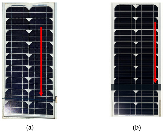
Figure 9.
The PV module covered with strips of ND filters replicating the constant-intensity ND filter shadow consisting of a single intensity, where (a) represents a coverage of 10% by the shaded strip on the PV module and (b) represents a fully shaded PV row with 100% coverage by the strip.
The sixth and seventh columns of Table 3 present the source values for the intensity attribute of both the dynamic-intensity and constant-intensity penumbra shadows. To replicate the intensity of the penumbra-only shadow, the gamma-corrected intensity values of each ND filter were categorised to correspond with the nearest matching penumbra-only instance. A visual example of a dynamic-intensity penumbra shadow and its corresponding constant-intensity shadow, matched in both size and average intensity, is shown with a red border in Figure 8a and Figure 8b, respectively. By closely matching both the size and intensity of the dynamic-intensity penumbra shadow, the constant-intensity shadow replicated using ND filter strips was applied to the small-scale PV module. The resulting power loss measurements are analysed using a regression model in Section 4.2 to evaluate the relationship between the two scenarios.
This regression model of best fit was employed to facilitate both visual interpretation and quantitative analysis. This approach enables a comparative assessment of the relationships and supports hypothesis testing through statistical metrics such as the coefficient of determination (R2) and residual analysis. Regression analysis is a widely accepted method for modelling relationships between variables, accounting for experimental variability and improving the reproducibility and interpretability of results, as demonstrated by Alshammari et al. [51] and Ayyub et al. [52]. Furthermore, statistical tests will also be applied to the regression models to numerically evaluate the significance of differences between the dynamic-intensity penumbra shadow and the constant-intensity ND filter shadow generated by the ND filters.
The results of the previously described methodology, encompassing both the preliminary and comparative analyses, are presented and discussed in Section 4.
4. Experimental Results
This section aims to provide empirical evidence, through a comparative analysis using the methodology outlined in Section 2, to determine whether there is a statistically significant difference between the dynamic-intensity penumbra shadow and the constant-intensity shadow. To illustrate the forthcoming sequence of results, Figure 10 presents an overview. The steps outlined in the methodology are highlighted with blue borders, while those that will be presented and discussed in this section are marked with red borders. The dashed lines imply shared use of figure, while arrows embody the flow within the methodology, from one stage to the next. As indicated by the blue-bordered elements, each respective dataset has been described, and a decision was made to use 29 penumbra-only instances from the prior work detailed in Ref. [26] as representative of the dynamic-intensity penumbra in the analysis that follows. Moreover, Section 4.1 details the preliminary experiments conducted to evaluate the effect of raising the ND filter from the PV module and to determine the intensity values associated with each ND filter. Section 4.2 then presents a comparative analysis between the dynamic-intensity penumbra shadow and constant-intensity shadow datasets, based on the 29 penumbra-only instances. Finally, a comprehensive statistical analysis is performed to assess the relationship and effect size between the two scenarios, ultimately determining whether to accept the null hypothesis (H0) or the alternative hypothesis (H1).
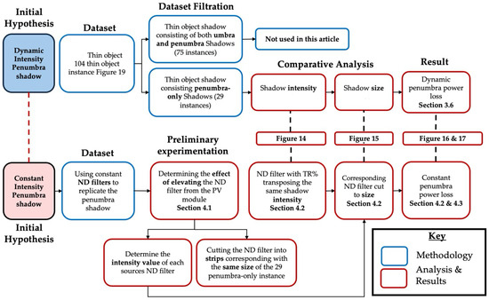
Figure 10.
Flowchart outlining the methodological steps illustrated by the blue border and the forthcoming results represented by the process with the red border, the figure labels refer to this research article except for Figure 19 in the dataset source flowchart box, which refers to [25].
4.1. Preliminary Experimental Measurements
The preliminary experimentation aims to assess two fundamental aspects of using ND filters on a PV module. First, it investigates whether elevating the ND filter at a distance of 50 cm from the surface of the PV module (detailed in Section 4.1.1) affects both the transposed shadow intensity and the resulting power loss when the entire module is shaded. Secondly, it seeks to determine the specific intensity value associated with each of the seven ND filters by capturing an image of the shadow cast on a white surface sheet.
4.1.1. Determining the Effect of Elevating the ND Filter from the PV Module
The TR 95% ND filter was selected as the filter under evaluation for this experiment. This is because it represents the highest transmission reduction level readily available on the market and produces the darkest shadow on the PV module, making it the most effective at uniformly reducing light across the entire surface. The filter was cut to match the exact dimensions of the PV module and positioned at heights ranging from 10 cm to 50 cm above the module, in 10 cm increments. Shadow intensity was measured using the ThinShadePV v1.1.1 tool, while power loss was quantified by calculating the percentage difference between the output of the control PV module and that of the experimental shaded module.
As shown in Table 4, the pixel intensity values (middle column) captured at all distances showed a level of consistency, indicating that varying the ND filter distance from the PV module up to 50 cm had no effect on the shadow intensity cast on the white surface sheet. This finding is particularly important, as Section 4.1.2 will determine the intensity values for all seven ND filters, which will then be used to replicate the intensities of the 29 penumbra-only instances. Additionally, the variation in power loss across all distances was minimal, with a maximum difference of only 0.43%. This negligible change demonstrates that elevating the ND filter up to 50 cm above the PV module during image capture neither affected the light intensity measurements nor compromised the accuracy of the data. These results provide a critical foundation for the subsequent experiments involving the characterisation of pixel intensity values for each sourced ND filter.
Table 4.
The resultant intensity level and power loss difference when elevating the ND filter from the PV module between 10 cm and 50 cm.
Following the results in Table 4, where no direct comparison with the dynamic-intensity penumbra shadow had been undertaken yet, the small-scale PV modules previously used in Ref. [26] were employed for the analysis in Section 4.2. These modules were ideal for facilitating a direct comparison between the dynamic-intensity penumbra shadow and the constant-intensity shadows, given that the baseline data for the dynamic-intensity penumbra shadow are sourced from prior work, as outlined in Ref. [26]. The continued use of the same PV module in Section 4.2 ensured experimental consistency by maintaining the same PV source throughout both the dynamic-intensity penumbra shadow and the constant-intensity shadow instances.
4.1.2. Determining the Intensity Value for the Range of ND Filters (on the White Surface Sheet)
Each of the seven ND filters listed in Table 2, and supported by the corresponding spectroscopy data shown in Figure 6, was positioned at 50 cm above a white surface sheet on top of the PV module. This setup mirrors the configuration previously illustrated in Figure 5b. Subsequently, an image was captured using the iPhone 15 portable camera described in Section 3.3 and then converted to 8-bit greyscale. Finally, using ThinShadePV, the intensity values were determined, and inverse gamma correction was applied (as explained at the end of Section 3.3).
Figure 11 depicts the results of both the original camera-captured intensity values and the corrected intensity values after inverse gamma correction. The orange line represents the raw intensity values captured by the iPhone camera, while the blue line shows the corresponding values after gamma correction. It is worth noting that certain intermediate TR levels (40, 70, and 80%) were not measured due to the unavailability of corresponding ND filters, representing a study limitation. To evaluate the accuracy of interpolating these missing levels, a sensitivity analysis was performed using a reduced calibration set of measured extremes (0% and 95%) and the interpolated intermediate levels. Intensities at withheld TR levels (10, 20, 30, and 50%) were then compared to measured values using monotone cubic interpolation. The intensity pixel value errors were low for camera-captured intensities (MAE = 2 pixels) and slightly higher for gamma-corrected intensities (MAE = 3 pixels), with the largest deviation at 20% TR (5 pixels) but ≤3 pixels for the remaining measured TR levels. This confirms that the interpolation of (40, 70, and 80%) introduces only minor pixel intensity errors. Nevertheless, the dynamic intensity will be compared only to the ND filters for which measurements were directly obtained, rather than to the interpolated values at 40, 70, and 80%. This was completed in order to ensure that the comparison is based on actual intensity readings and is not affected by interpolation errors.
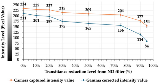
Figure 11.
The image captured intensity (orange) and the gamma-corrected pixel intensity values (blue) plotted against each ND filter TR level sourced.
An initial observation reveals that the rate of change between the original intensity values and the gamma-corrected values is not constant. This is because the gamma correction formula, as previously defined in Equation (2), represents a non-linear transformation. As a result, equal increments in input intensity do not produce equal changes in the output.
It is evident that the raw intensity values illustrated by the orange line in Figure 11 shift downwards due to a pixel intensity decrease with increasing TR%, providing a more accurate representation of real-world intensity values as compared to the camera-captured intensity values. Taken as a baseline measurement prior to applying any ND filter to the PV module, the observed intensity at 0% TR does not reach the maximum possible pixel intensity of 255. Instead, the camera-captured intensity measures 234, while the gamma-corrected value is 211. This deviation may be attributed to internal iPhone camera exposure settings designed to prevent sensor saturation, transmission losses through optical components, or the reflectance properties of the white surface sheet used. The white surface sheet is important to create a baseline contrast as a background intensity value to attenuate the shadow in question in the image capture. As the TR level increases across the x-axis, the decline in intensity follows a non-linear trend, with a significantly sharper drop observed beyond the 75% TR level. For example, the gamma-corrected intensity decreases from 156 at 75% TR to 84 at 95% TR, indicating substantial sensitivity to light attenuation at higher TR percentages. This behaviour can be attributed to the camera sensor’s limited response under low-light conditions, as discussed by Rezagholizadeh et al. [53]. At these darker levels, photon noise and read noise become more pronounced, and the sensor’s response becomes less consistent. This non-linearity is further amplified by the gamma correction process, which disproportionately affects lower intensity values due to its exponential nature. As such, applying gamma correction is essential when working with variable lighting conditions to ensure accurate intensity measurements.
It is notable that, when using ND filters having a TR of 95%, the camera captured pixel intensity is observed to have the lightest recorded pixel value of 154. The gamma-corrected intensity of the same ND filter reduces the value from 154 to 84, incurring a difference of a 70 pixel value. Comparatively, the 70 pixel value difference is almost three times the difference between the baseline pixel values at 0% TR, where a 23 pixel value difference was observed. This difference is significant, and a pixel value of 84 is considerably darker in nature when referring to the 0–255 scale on the left side of Figure 11. Therefore, to compare dynamic-intensity penumbra shadows with constant-intensity shadows, the subsequent section will also need to determine which of the gamma-corrected pixel intensity values correspond to the penumbra-only shadow being replicated.
4.2. Experimental Procedure
Building on the preliminary experimental results discussed in Section 4.1, this section directly addresses the hypothesis introduced at the end of Section 1. The objective is to replicate the size and intensity of the 29 penumbra-only thin-object shading instances extracted from prior work outlined in Ref. [26], using ND filters, as described in the methodology in Section 3.4. The analysis then compares the power loss between these 29 dynamic-intensity penumbra-only shadow instances and their corresponding constant-intensity shadow, which is created using the various TR levels of ND filters employed in this article.
Firstly, the power loss across the 29 penumbra-only instances was illustrated in Figure 12. The object thicknesses of the 29 instances ranged from ⌀3.2 mm to ⌀12 mm at distances beginning at 175 cm and extending until the shadow covers the whole solar cell area at a maximum limit of 375 cm. Beyond a thickness of ⌀12 mm, the thin objects were observed to produce either a predominantly umbra shadow or, during the transition to penumbra, generate a shadow that exceeds the surface width of the solar cell. Therefore, if either of the latter two observations was noted, the respective shadow instances were not considered as penumbra-only shadows and were discarded as previously visualised in Figure 10. To visualise an exemplary penumbra-only shadow, Figure 13a demonstrates an instance where the shadow is dynamic in intensity, in contrast with the shadow produced by the ND filters in Figure 13b. The procedure to determine the size and averaged intensity of each shadow will be replicated for all 29 dynamic-intensity shadow instances as previously explained in Section 3.4 and more specifically in Table 3. The uncertainty for each power loss value is given as an average uncertainty of ±2.29%.
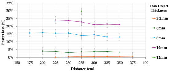
Figure 12.
The extracted power loss from each of the 29 dynamic-intensity penumbra-only instances, detailed in prior work outlined in Ref. [26].
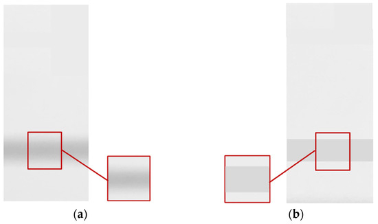
Figure 13.
(a) A penumbra-only shadow created by the thin object; (b) the constant-intensity shadow using ND filter strips.
The first main attributing factor of the penumbra-only shadows is the intensity of the shadow of the 29 instances. Mapping was performed between the intensity values of the seven ND filters shown in Figure 11 and the dynamic-intensity values represented by the blue curve in Figure 14. This mapping aimed to identify the closest corresponding transmittance percentage (TR%) for each dynamic-intensity shadow instance, thereby aligning each of the 29 dynamic-intensity shadows with a comparable constant-intensity shadow. This approach ensured that the intensity levels being compared were closely matched, enabling a comparison of the bases of the attributing factors of a shadow for the subsequent analysis.
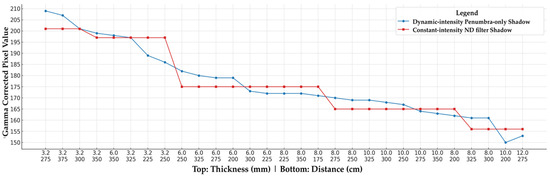
Figure 14.
A graph comparing the gamma-corrected intensity values of the 29 penumbra-only instances represented as the dynamic-intensity penumbra-only shadow in blue and the constant-intensity ND filter intensities shown in red.
The blue line in Figure 14 illustrates the intensity values of each of the 29 penumbra-only instances, sorted in descending order from the highest to lowest gamma-corrected intensity value. The lightest intensity instance observed from the 29 penumbra-only instances was a pixel value of 209, shown as the first left-hand side point on the blue line of Figure 14. Referring to the gamma-corrected blue line previously shown in Figure 11, the closest intensity value corresponding to the 209 pixel value generated by an ND was 10% TR (excluding the 0% TR no shadow), demonstrating an intensity of 201. With just an 8 pixel value difference from the lightest pixel intensity of the 29 instances, the TR 10% will be the upper limit to replicate the penumbra-only intensity of the 29 instances.
On the other hand, the darkest penumbra-only instance recorded in Figure 14 produced an intensity value of 153. The closest matching TR level in Figure 11 was 75%, producing an intensity of 156. Therefore, a TR level of 75% was selected as the lower bound for replicating penumbra-only intensity values. Higher TR levels, such as at 90% and 95%, produced much darker intensities of 114 and 84, respectively, well below the penumbra-only range, and were thus deemed too dark to accurately replicate any of the 29 penumbra-only instances.
Consequently, TR levels of 10, 20, 30, 50, and 75% were found to fall within the appropriate intensity range for replication. The intensity of these five ND filters, previously shown in Figure 11, was each matched (binned) to the closest corresponding intensity values from the 29 penumbra-only instances. This mapping is illustrated in Figure 14, where the penumbra-only instances are denoted in blue, and the binned ND filter intensities are shown in red, demonstrating close alignment. The maximum pixel difference between the two categories was 11, and the minimum was 0. These results confirm that the five selected ND filters successfully replicated the intensity range of the 29 penumbra-only shadow instances with an acceptable accuracy.
The second defining attributing factor of the penumbra-only shadow is its size. It is essential that the replicated constant-intensity shadow closely matches the area coverage of the 29 penumbra-only instances. In Figure 15, the blue scatter plot represents the percentage area coverage of the solar cell for all 29 penumbra-only instances extracted from prior thin-object shading instance power loss results from [26]. The five ND filters, which were binned to the 29 penumbra-only intensities demonstrated in Section 4.2, were employed in this section to replicate these shadow instances. These ND filters were cut into strips closely matching the dimensions of the original penumbra-only instances, implementing the methodology described in Section 3.4. The corresponding percentage coverage for each ND filter strip is represented by the red scatter points in Figure 15, which closely align with the blue scatter points representing the 29 dynamic-intensity penumbra shadows. The analysis revealed a maximum difference of +4.98%, a minimum difference of −4.98%, and an average difference of approximately −0.36% between the two datasets. These results indicate that the ND filters produced shadows with solar cell area coverage acceptably similar to that of the penumbra-only instances, complementing the previous outcomes in Section 4.2 with regard to intensity.
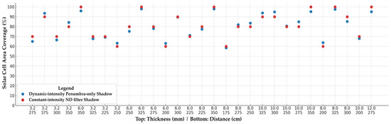
Figure 15.
Comparison of percentage area covered by the shadow on the solar cell for the dynamic-intensity penumbra-only shadow and the constant-intensity shadow produced from the ND filter strips.
With size and intensity successfully replicated to an acceptable rate of accuracy, as seen in Figure 14 and Figure 15, respectively, the ND filters were subsequently placed on top of the PV module in the middle of the solar cell, as visualised in Figure 5 and the setup presented in Figure 8. The power loss difference between the control and experimental PV modules, at identical calibrated power outputs, was subsequently retrieved from the constant-intensity shadows created on the PV module. A comparison of the percentage power loss between the dynamic-intensity penumbra-only shadow and the constant-intensity shadow created by the ND filters is visualised in Figure 16.
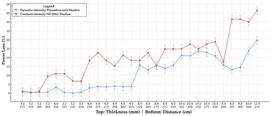
Figure 16.
Comparison of the percentage power loss for the dynamic-intensity penumbra-only shadow and the constant-intensity shadows created by the ND filters.
Figure 16 reveals a clear discrepancy in power loss between the two shading conditions. A comparative analysis between Dynamic and Constant Penumbra Power Loss revealed a maximum difference of +0.38% power loss, a minimum difference of −28.46% power loss, and an average difference of −9.65% power loss. In almost all cases, the constant-intensity ND filter shadow resulted in greater power loss when compared to the dynamic-intensity penumbra-only shadow. This suggests that, even when the size and intensity of both types of shadows are aligned, the constant-intensity ND shadow imposed a more pronounced negative impact on the PV module’s performance. Furthermore, despite the differences in magnitude, a similar trend between the power loss percentage of dynamic-intensity penumbra and constant-intensity shadows can be observed in Figure 16. This indicates a potential underlying relationship warranting further statistical analysis to determine its consistency and to assess the significance of the observed power loss differences. Consequently, Section 4.3 shall further elaborate our analysis, making use of regression models to comprehend the relationships and trends between the dynamic- and constant-intensity shadows.
4.3. Results and Interpretation
Regression models were utilised to investigate the relationship and magnitude between the dynamic-intensity shadow and the constant-intensity shadow produced by the ND filters. The primary aim was to quantify observable trends and assess the statistical significance of variations in shadow behaviour under differing intensity conditions. These are represented in Figure 17. The dynamic-intensity penumbra shadow is shown as a blue dotted polynomial curve, and the constant-intensity shadow is represented by the red dotted curve.
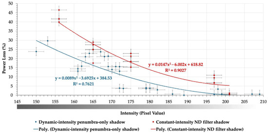
Figure 17.
Comparison between dynamic-intensity shadow and constant-intensity shadow created by ND filters.
For both shadow types, a second-degree polynomial regression model was fitted to evaluate the predictive relationship between percentage power loss and pixel intensity values. This model type was chosen as it adequately captured the curvature present in dynamic-intensity penumbra-only and constant-intensity ND filter shadows, yielding a higher coefficient of determination (R2 > 0.75) than third and fourth-degree polynomials (R2 < 0.62). The inferior performance of higher-order models was attributed to Runge’s phenomenon, which introduces oscillations that undermine fitting reliability [54]. Polynomial regression was further preferred for its interpretable coefficients, in contrast to non-parametric models that characterise data shape without providing explicit parameters.
To assess the predictive accuracy of each model, model error analysis was conducted using MAE and RMSE. The dynamic-intensity penumbra shadow model achieved an MAE of 3.74% and an RMSE of 4.43%, while the constant-intensity ND filter shadow model achieved an MAE of 2.92% and an RMSE of 3.72%. These results indicate that both regression models represent the power loss data points for both shadow types effectively and are adequate for the subsequent statistical analysis.
An initial comparison of the two regression models reveals that their overall trends are relatively similar, a consistency attributed to the close replication of both penumbra shadow size and intensity. However, a distinct difference in the power loss regression models of Figure 17 is evident. To further investigate this, a statistical analysis was performed to evaluate the relationship between the two models, to assess the significance of the observed power loss differences, and to quantify the predictive errors associated with each model. A summary of these results is provided in Table 5 and discussed subsequently.
Table 5.
Comparative summary of model fit, group statistical differences, and prediction errors for the dynamic-intensity penumbra-only shadow and the constant-intensity ND shadows.
Both the dynamic-intensity penumbra-only shadow and the constant-intensity ND filter shadow exhibit the clear trend that, when shadow intensity decreases, power loss also diminishes across all 29 instances. Both models exhibit positive quadratic coefficients, reflecting the downward-sloping, curved trends observed in the graph. The constant-intensity shadow shows a slightly steeper decline and more pronounced curvature, as evidenced by its larger absolute linear and quadratic coefficients. In addition, the model representing the constant-intensity shadow achieved a slightly better fit, with a lower mean absolute error (2.92 compared to 3.74) and a higher R2 value (0.903 vs. 0.762). Adjusted R2 values (0.895 vs. 0.743) further confirm that the constant-intensity ND regression model retains a stronger explanatory power even after accounting for the number of predictors. Despite these differences, the similarity in the curvature of the two models suggests a broadly comparable trend between intensity and power loss. However, while the models visually appear similar, further detailed statistical analysis is required to conclusively determine the statistical significance of the magnitude of power loss between the two shadow conditions.
To assess the normality of the percentage dynamic power loss data, both statistical and visual methods were applied. The Shapiro–Wilk test yielded a p-value of 0.0032, indicating a statistically significant deviation from normality (p < 0.05). This conclusion is further supported by visual inspection through a histogram plot of the power loss, which revealed clear left-skewness and deviation from the normal curve. Therefore, since the traditionally used Welch t-test must satisfy the normality assumption, it cannot be used as the Shapiro–Wilk test results in non-normally distributed data, as is the case in this section. Alternatively, West [55] suggests the use of the Mann–Whitney U-test, which is almost as powerful and has no distributional assumptions. Oti et al. [56] and Fang [57] demonstrated the effectiveness of the Mann–Whitney U-test in anomaly detection for non-normally distributed data, highlighting its advantages over parametric methods, specifically in complex PV fault detection scenarios. Building on this, Yang and Fang [57] introduced a non-linear fault detection model using the Mann–Whitney test, achieving improved accuracy by reducing false positives and missed faults, thus reinforcing its robustness in complex PV fault detection scenarios. Therefore, the Mann–Whitney U-test was performed for the two groups of shadows, yielding a statistically significant difference between the groups (p = 0.00229). Assumptions required for these tests, including variance equality (Levene’s test, p = 0.542) and sample size adequacy (small sample size required), were checked and satisfied.
Moreover, apart from the significance p-value, research conducted by Sullivan et al. [58] and Lakens [59] denoted that the ‘effect size’ helps in understanding the magnitude of differences found, whereas statistical significance examines whether the findings are likely to be due to chance. In this way, the Cohen’s d-test was chosen to determine the effect size, complementing the significance level between both dynamic-intensity penumbra shadow and constant-intensity shadow groups. The magnitude of this difference was quantified using Cohen’s d, which yielded a value of −0.893, reflecting a large effect size and strong practical significance.
These results strongly suggest that the type of shadow has a statistically and practically significant impact on power loss. Nevertheless, although the curvature of the models representing the relationship between intensity and power loss is visually similar between the two shadow types, the constant-intensity ND shadow does not produce the same power loss effect on a PV source, even though both intensity and size are kept relatively the same. Constant-intensity shading, typically caused by fixed structures, produces a stable and uniform shadow intensity, which is well represented in standard irradiance models and commercial PV simulation tools, as exemplified by Grover et al. [60], Chedid et al. [61], and Ramadan et al. [62]. In comparison, dynamic penumbra, often introduced by thin, elevated objects such as overhead wires or poles, results in variable and spatially uneven shading across PV modules. This variability can lead to localised mismatch effects, especially when varying the distance between the shading object and the PV source. If these dynamic effects are not distinguished from constant shading, performance estimates may become less reliable, potentially affecting design decisions and system generation expectations. Recognising the characteristics of dynamic shading can support more appropriate design strategies, including the configuration of module strings and the use of maximum power point tracking techniques by PV designers and technicians in the field. The inclusion of the constant and dynamic shadow distinction in PV simulation modelling can clearly contribute to more accurate quantification of PV losses.
5. Conclusions
A direct comparison of the 29 penumbra-only shadow instances of dynamic-intensity and the replicated constant-intensity shadows indicated that the curvature of the power loss versus intensity models appeared visually similar, as reflected in the high R2 values of 0.762 and 0.903 for the dynamic-intensity penumbra and constant-intensity models, respectively. Contrastingly, detailed statistical analysis revealed that, even though the relationships of both models were similar, the constant-intensity ND shadow produces an average of 9.64% more power loss than the dynamic-intensity shadow. This was also confirmed statistically with the Mann–Whitney U-test (p = 0.00229). Consequently, based on the experimental results, the null hypothesis (H0), which stated that there is no statistically significant difference in power loss between dynamic-intensity penumbra shadow and constant-intensity shadows, was rejected. The alternative hypothesis (H1) was accepted, indicating that the dynamic characteristics of the penumbra do significantly influence PV performance. These findings demonstrate that simplifying the penumbra to a constant-intensity shadow introduces a measurable deviation in power output.
6. Limitations and Future Work
A notable limitation of using ND filtering materials is that, although a total of seven ND filters were sourced for this study, only five fell within the specific intensity range necessary for the direct comparison with penumbra-only instances. This limited selection contributed to the wider spacing observed between the red data points in Figure 17. Future work should aim to incorporate a broader range of ND filters specifically within the penumbra-only intensity range to enable a more comprehensive and precise comparison, thereby improving model fidelity.
A key limitation of this study is the restriction to single-layer ND filters due to the absence of peer-reviewed validation for the transmittance behaviour of stacked filters. While stacking ND filters could offer more precise control over gradient shadowing, potential issues such as spectral distortion, non-uniform attenuation, and cumulative optical effects introduced uncertainties that were beyond the scope of this work. Future research should investigate the optical properties and transmission consistency of stacked ND filters under controlled conditions, which could enhance the accuracy of penumbra simulation and broaden the applicability of the methodology.
Author Contributions
Conceptualization, M.A., L.M.S. and M.D.; methodology, M.A., L.M.S. and M.D.; validation, M.A., M.D. and L.M.S.; Investigation, M.A.; formal analysis, M.A., L.M.S. and M.D.; resources, M.A., L.M.S. and M.D.; writing—original draft preparation, M.A.; writing—review and editing, L.M.S. and M.D.; supervision, L.M.S. and M.D.; project administration, L.M.S. and M.D. All authors have read and agreed to the published version of the manuscript.
Funding
This research received no external funding.
Institutional Review Board Statement
The study abided by the University of Malta’s research ethics review procedures. Furthermore, the University of Malta’s Research Ethics ApplicationID ENG-2024-00038 covers the research ethics approvals for this research article.
Data Availability Statement
The data presented in this study are available on request from the corresponding author.
Conflicts of Interest
The authors declare no conflicts of interest.
References
- Aljumaili, M.; Abdalkafor, A.; Taha, M. Analysis of the Hard and Soft Shading Impact on Photovoltaic Module Performance Using Solar Module Tester. Int. J. Power Electron. Drive Syst. 2019, 10, 1015. [Google Scholar] [CrossRef]
- Numan, A.H.; Dawood, Z.S.; Hussein, H.A. Theoretical and experimental analysis of photovoltaic module characteristics under different partial shading conditions. Int. J. Power Electron. Drive Syst. 2020, 11, 1508. [Google Scholar] [CrossRef]
- Teneta, J.; Kreft, W.; Janowski, M. Partial Shading of Photovoltaic Modules with Thin Linear Objects: Modelling in MATLAB Environment and Measurement Experiments. Energies 2024, 17, 3546. [Google Scholar] [CrossRef]
- Dolara, A.; Lazaroiu, G.C.; Leva, S.; Manzolini, G. Experimental investigation of partial shading scenarios on pv (photovoltaic) modules. Energy 2013, 55, 466–475. [Google Scholar] [CrossRef]
- Sinapis, K.; Litjens, G.; Donker, M.; Folkerts, W.; Sark, W. Outdoor characterization and comparison of string and mlpe under clear and partially shaded conditions. Energy Sci. Eng. 2015, 3, 510–519. [Google Scholar] [CrossRef]
- Dhimish, M.; Theristis, M.; d’Alessandro, V. Photovoltaic hotspots: A mitigation technique and its thermal cycle. Optik 2024, 300, 171627. [Google Scholar] [CrossRef]
- Numan, A.; Hussein, H.A.; Dawood, Z.S. Hot Spot Analysis of Photovoltaic Module under Partial Shading Conditions by Using IR-Imaging Technology. Eng. Technol. J. 2021, 39, 1338–1344. [Google Scholar] [CrossRef]
- Fri, A.; El Bachtiri, R.; El Ghzizal, A. Improved MPPT Algorithm for Controlling a PV System Grid Connected for Rapid Changes of Irradiance. Int. Rev. Autom. Control IREACO 2016, 9, 11. [Google Scholar] [CrossRef]
- Shankar, N.; SaravanaKumar, N. Reduced Partial shading effect in Multiple PV Array configuration model using MPPT based Enhanced Particle Swarm Optimization Technique. Microprocess. Microsyst. 2020, 103287. [Google Scholar] [CrossRef]
- Ismail, M.A.; Adil, N.L.J.; Yan, F.Y.; Amaludin, N.; Bohari, N.; Sar-ee, S. Analysis of the Effects of Hard Shading Pattern on I–V Performance Curve. Appl. Sol. Energy 2023, 59, 369–377. [Google Scholar] [CrossRef]
- Klugmann-Radziemska, E. Shading, Dusting and Incorrect Positioning of Photovoltaic Modules as Important Factors in Performance Reduction. Energies 2020, 13, 1992. [Google Scholar] [CrossRef]
- Liu, Z.; Huang, K.; Tan, T.; Wang, L. Cast Shadow Removal with GMM for Surface Reflectance Component. In Proceedings of the 18th International Conference on Pattern Recognition (ICPR’06), Hong Kong, China, 20–24 August 2006; p. 730. [Google Scholar]
- Hernán, J. Calculation of the shadow-penumbra relation and its application on efficient architectural design. Sol. Energy 2014, 110, 139–150. [Google Scholar] [CrossRef]
- Luo, C.; Wu, Y.; Su, X.; Zou, W.; Yu, Y.; Jiang, Q.; Xu, L. Influence and characteristic of shading on photovoltaic performance of bifacial modules and method for estimating bifacial gain. In Building Simulation; Tsinghua University Press: Beijing, China, 2023. [Google Scholar] [CrossRef]
- Bae, J.; Jee, H.; Park, Y.; Lee, J. Simulation-Based Shading Loss Analysis of a Shingled String for High-Density Photovoltaic Modules. Appl. Sci. 2021, 11, 11257. [Google Scholar] [CrossRef]
- Feng, X.; Ma, T. Solar Photovoltaic system under partial shading and perspectives on maximum utilization of the shaded land. Int. J. Green Energy 2023, 20, 378–389. [Google Scholar] [CrossRef]
- Zandi, Z.; Mazinan, A.H. Maximum power point tracking of the solar power plants in shadow mode through artificial neural network. Complex Intell. Syst. 2019, 5, 315–330. [Google Scholar] [CrossRef]
- Gutiérrez Galeano, A.; Bressan, M.; Jiménez Vargas, F.; Alonso, C. Shading Ratio Impact on Photovoltaic Modules and Correlation with Shading Patterns. Energies 2018, 11, 852. [Google Scholar] [CrossRef]
- Wang, Z.; Zhou, Y.; Wang, F.; Wang, S.; Qin, G.; Zhu, J. Shadow Detection and Reconstruction of High-Resolution Remote Sensing Images in Mountainous and Hilly Environments. IEEE J. Sel. Top. Appl. Earth Obs. Remote Sens. 2024, 17, 1233–1243. [Google Scholar] [CrossRef]
- Murali, S.; Govindan, V.K.; Kalady, S. A Survey on Shadow Detection Techniques in a Single Image. Inf. Technol. Control 2018, 47, 75–92. [Google Scholar] [CrossRef]
- Dendrinos, D. On the Fuzzy Nature of Shadows. 2017. Available online: https://www.researchgate.net/profile/Dimitrios-Dendrinos/publication/317433717_ON_THE_FUZZY_NATURE_OF_SHADOWS/links/593aa58ba6fdcc17a9898705/ON-THE-FUZZY-NATURE-OF-SHADOWS.pdf (accessed on 5 February 2025).
- Geometrical Optics Laboratory. Available online: https://www.animations.physics.unsw.edu.au/labs/geometrical-optics/geometrical-optics-lab.html (accessed on 7 January 2025).
- Ramanath, R.; Drew, M.S. Penumbra and Umbra. In Computer Vision: A Reference Guide; Ikeuchi, K., Ed.; Springer: Boston, MA, USA, 2014; pp. 589–590. ISBN 978-0-387-31439-6. [Google Scholar]
- Axisa, M.; Demicoli, M.; Mule’Stagno, L. Analysing the Effects of Thin Object Shading on PV Sources: A Dual Approach Combining Outdoor and Laboratory Solar Simulator Experimentation. Energies 2024, 17, 2069. [Google Scholar] [CrossRef]
- Axisa, M.; Mule’Stagno, L.; Demicoli, M. Quantifying the effect of shadow formation on photovoltaic sources under thin object shading: An image analysis approach. EPJ Photovolt. 2025, 16, 17. [Google Scholar] [CrossRef]
- Axisa, M.; Mule’Stagno, L.; Demicoli, M. Correlating field experimentation and image analysis for the assessment of induced losses from thin object shading on photovoltaic sources. In Proceedings of the EU PVSEC 2024, Vienna, Austria, 23–27 September 2024. [Google Scholar]
- De Rosa, A.; Bortot, A.; Bergamo, F. Praise of Penumbra; John Wiley & Sons: Hoboken, NJ, USA, 2023; ISBN 1-119-98396-7. [Google Scholar]
- Štampfl, V.; Gabrijelčič, H.; Ahtik, J. The Role of Light and Shadow in the Perception of Photographs. Teh. Vjesn. 2023, 30, 1347–1356. [Google Scholar] [CrossRef]
- Serrano, M.-A.; Moreno, J.C. Spectral transmission of solar radiation by plastic and glass materials. J. Photochem. Photobiol. B 2020, 208, 111894. [Google Scholar] [CrossRef]
- Duarte, I.; Rotter, A.; Malvestiti, A.; Hafner, M. The role of glass as a barrier against the transmission of ultraviolet radiation: An experimental study. Photodermatol. Photoimmunol. Photomed. 2009, 25, 181–184. [Google Scholar] [CrossRef] [PubMed]
- Littlejohn, B.; Heeger, K.; Wise, T.; Gettrust, E.; Lyman, M. UV degradation of the optical properties of acrylic for neutrino and dark matter experiments. J. Instrum. 2009, 4, T09001. [Google Scholar] [CrossRef]
- Simonot, L.; Hébert, M.; Mazauric, S.; Hersch, R.D. Assessing the proper color of translucent materials by an extended two-flux model from measurements based on an integrating sphere. Electron. Imaging 2017, 2017, 48–56. [Google Scholar] [CrossRef]
- Kalyani, V.; Sharma, V. Different types of Optical Filters and their Realistic Application. J. Manag. Eng. Inf. Technol. 2016, 3, 12–17. [Google Scholar]
- Lam, E.Y.; Fung, G.S.K. Automatic white balancing in digital photography. In Single-Sensor Imaging: Methods and Applications for Digital Cameras; CRC Press: Boca Raton, FL, USA, 2008; pp. 267–294. [Google Scholar]
- Heron, G.; Dutton, G.N. The Pulfrich phenomenon and its alleviation with a neutral density filter. Br. J. Ophthalmol. 1989, 73, 1004. [Google Scholar] [CrossRef]
- Murakami Color Research Laboratory. ND Filter. Available online: https://www.mcrl.co.jp/english/products/p_standard/detail/NDfilters.html (accessed on 18 January 2025).
- Kase Filters. Using Graduated ND Filters. Available online: https://kasefilters.eu/nice-to-know/guides/using-graduated-nd-filters/ (accessed on 15 January 2025).
- Willey, R. Designing Metallic Neutral Density Filters with Constant Optical Density Versus Wavelength. Space Sci. J. 2024, 1, 1–7. [Google Scholar] [CrossRef]
- Figueiredo Ramos, C.A.; Alcaso, A.; Cardoso, A.J.M. Photovoltaic-thermal (PVT) technology: Review and case study. IOP Conf. Ser. Earth Environ. Sci. 2019, 354, 012048. [Google Scholar] [CrossRef]
- Shelby, J.E. OPTICAL MATERIALS|Color Filter and Absorption Glasses. In Encyclopedia of Modern Optics; Guenther, R.D., Ed.; Elsevier: Oxford, UK, 2005; pp. 440–446. ISBN 978-0-12-369395-2. [Google Scholar]
- Luciani, S.; Coccia, G.; Tomassetti, S.; Pierantozzi, M.; Di Nicola, G. Correction Procedures for Temperature and Irradiance of Photovoltaic Modules: Determination of Series Resistance and Temperature Coefficients by Means of an Indoor Solar Flash Test Device. Tec. Ital.-Ital. J. Eng. Sci. 2021, 65, 264–270. [Google Scholar] [CrossRef]
- IEC 60904-1:2020; Part 1: Measurement of Photovoltaic Current-Voltage Characteristics. International Standard: Geneva, Switzerland, 2020.
- Understanding Neutral Density Filters|Edmund Optics. Available online: https://www.edmundoptics.com/knowledge-center/application-notes/optics/understanding-neutral-density-filters/?srsltid=AfmBOorwBdA2g5zdwLEDddyzul6popAOdCHe_N_jGyJezKwTqgpO72Dj (accessed on 8 May 2025).
- Sinapis, K.; Tzikas, C.; Litjens, G.; van den Donker, M.; Folkerts, W.; van Sark, W.G.J.H.M.; Smets, A. A comprehensive study on partial shading response of c-Si modules and yield modeling of string inverter and module level power electronics. Sol. Energy 2016, 135, 731–741. [Google Scholar] [CrossRef]
- Bognár, Á.; Loonen, R.C.G.M.; Valckenborg, R.M.E.; Hensen, J.L.M. An unsupervised method for identifying local PV shading based on AC power and regional irradiance data. Sol. Energy 2018, 174, 1068–1077. [Google Scholar] [CrossRef]
- Khobragade, K. A Comparative study of Converting Coloured Image to Gray-scale Image using Different Technologies. Master’s Thesis, Fergusson College, Pune, India, 2012. [Google Scholar]
- Soni, S.; Singh, P.; Waoo, A. Review of gamma correction techniques in digital imaging. ShodhKosh J. Vis. Perform. Arts 2024, 5, 473–479. [Google Scholar] [CrossRef]
- Singnoo, J.; Finlayson, G. Understanding the Gamma Adjustment of Images. In Proceedings of the Color and Imaging Conference, San Antonio, TX, USA, 8–12 November 2010. [Google Scholar]
- Carlos, J.; Fernandes, J.C. Linear versus Non-Linear Digital Image Processing Methods. In Proceedings of the Congresso Luso-Moçambicano de Engenharia, Maputo, Moçambique, 29 July–2 August 2025. [Google Scholar]
- Farid, H. Blind inverse gamma correction. IEEE Trans. Image Process. 2001, 10, 1428–1433. [Google Scholar] [CrossRef]
- Alshammari, A. Implementation of Curve Fitting using Polynomial Regression in Python. Int. J. Comput. Appl. 2024, 186, 27–32. [Google Scholar] [CrossRef]
- Ayyub, B.; Mccuen, R. Curve Fitting and Regression Analysis. In Numerical Analysis for Engineers; CRC: Boca Raton, FL, USA, 2015; pp. 331–394. ISBN 978-0-429-16212-1. [Google Scholar]
- Rezagholizadeh, M.; Clark, J. Image Sensor Modeling: Color Measurement at Low Light Levels. In Proceedings of the Color and Imaging Conference, Boston, MA, USA, 3–7 November 2014; Volume 58. [Google Scholar]
- Udo, O.C.; Idochi, O. Simple Regression Models: A Comparison using Criteria Measures. Afr. J. Math. Stat. Stud. 2024, 7, 131–143. [Google Scholar] [CrossRef]
- West, R.M. Best practice in statistics: Use the Welch t-test when testing the difference between two groups. Ann. Clin. Biochem. 2021, 58, 267–269. [Google Scholar] [CrossRef] [PubMed]
- Oti, E.U.; Olusola, M.O.; Esemokumo, P.A. Statistical Analysis of the Median Test and the Mann-Whitney U Test. Int. J. Adv. Acad. Res. 2021, 7, 44–51. [Google Scholar]
- Yang, C.; Fang, H. A New Nonlinear Model-Based Fault Detection Method Using Mann–Whitney Test. IEEE Trans. Ind. Electron. 2020, 67, 10856–10864. [Google Scholar] [CrossRef]
- Sullivan, G.M.; Feinn, R. Using Effect Size—Or Why the P Value Is Not Enough. J. Grad. Med. Educ. 2012, 4, 279–282. [Google Scholar] [CrossRef]
- Lakens, D. Calculating and reporting effect sizes to facilitate cumulative science: A practical primer for t-tests and ANOVAs. Front. Psychol. 2013, 4, 863. [Google Scholar] [CrossRef] [PubMed]
- Grover, A.; Khosla, A.; Joshi, D. Design and simulation of 20MW photovoltaic power plant using PVSyst. Indones. J. Electr. Eng. Comput. Sci. 2020, 19, 58. [Google Scholar] [CrossRef]
- Chedid, R.; Tajeddine, R.; Chaaban, F.; Ghajar, R. Modeling and simulation of PV arrays under varying conditions. In Proceedings of the MELECON 2014-2014 17th IEEE Mediterranean Electrotechnical Conference, Beirut, Lebanon, 13–16 April 2014; p. 542. [Google Scholar]
- Ramadan, A. Rooftop solar PV system planning with 3D visualization using PVSOL (Case study in Syria). J. Sci. Eng. Res. 2024, 11, 66–77. [Google Scholar]


Disclaimer/Publisher’s Note: The statements, opinions and data contained in all publications are solely those of the individual author(s) and contributor(s) and not of MDPI and/or the editor(s). MDPI and/or the editor(s) disclaim responsibility for any injury to people or property resulting from any ideas, methods, instructions or products referred to in the content. |
© 2025 by the authors. Licensee MDPI, Basel, Switzerland. This article is an open access article distributed under the terms and conditions of the Creative Commons Attribution (CC BY) license (https://creativecommons.org/licenses/by/4.0/).