CNN Input Data Configuration Method for Fault Diagnosis of Three-Phase Induction Motors Based on D-Axis Current in D-Q Synchronous Reference Frame

Abstract

This study proposes a novel approach to input data configuration for the fault diagnosis of three-phase induction motors. Conventional neural network (CNN)-based diagnostic methods often employ three-phase current signals and apply various image transformation techniques, such as RGB mapping, wavelet transforms, and short-time Fourier transform (STFT), to construct multi-channel input data. While such approaches outperform 1D-CNNs or grayscale-based 2D-CNNs due to their rich informational content, they require multi-channel data and involve an increased computational complexity. Accordingly, this study transforms the three-phase currents into the D-Q synchronous reference frame and utilizes the D-axis current (Id) for image transformation. The Id is used to generate input data using the same image processing techniques, allowing for a direct performance comparison under identical CNN architectures. Experiments were conducted under consistent conditions using both three-phase-based and Id-based methods, each applied to RGB mapping, DWT, and STFT. The classification accuracy was evaluated using a ResNet50-based CNN. Results showed that the Id-STFT achieved the highest performance, with a validation accuracy of 99.6% and a test accuracy of 99.0%. While the RGB representation of three-phase signals has traditionally been favored for its information richness and diagnostic performance, this study demonstrates that a high-performance CNN-based fault diagnosis is achievable even with grayscale representations of a single current.

1. Introduction

To enhance the reliability and maintenance efficiency of three-phase induction motors, which are widely used in modern industrial environments, various fault diagnosis techniques have been actively researched. These techniques can be broadly categorized into model-based approaches grounded in signal processing and data-driven approaches utilizing artificial intelligence (AI).

Among model-based methods, representative techniques include fast Fourier transform (FFT) for frequency domain analysis, D-Q transformation for converting time-series data into a fixed reference frame, and Park’s vector analysis [1,2,3]. In particular, the D-Q transformation using Park’s vector allows three-phase current data to be represented on two axes (Id and Iq). Among these, the Id-axis current reflects the motor’s magnetic flux component and offers advantages such as simplified analysis, elimination of phase imbalance, and reduced sensitivity to noise [2,3]. Consequently, many studies have suggested that using only the Id-axis signal obtained through D-Q transformation enables a simple yet reliable fault diagnosis, in contrast to directly analyzing the original three-phase signals.

Recently, data-driven fault diagnosis methods using convolutional neural networks (CNNs) have gained considerable attention. As CNNs demonstrate excellent performance when processing visually structured data, various studies have transformed three-phase current signals into image formats suitable for CNN input. Typical approaches involve direct RGB mapping of the three-phase currents or applying transformations such as the discrete wavelet transform (DWT) and short-time Fourier transform (STFT) to create RGB image representations, which are then used for fault classification via CNN models [4,5,6].

These RGB-based methods have been reported to provide a significantly better diagnostic performance than grayscale or 1D time-series inputs [7,8]. However, most prior studies utilized all three-phase current signals, which inherently increases the computational complexity due to inter-phase variations and noise.

To address this limitation, the present study draws inspiration from the model-based diagnosis literature, which highlights the benefits of using the Id current component. The aim is to experimentally verify whether a comparable diagnostic performance can be achieved in CNN-based fault detection using only the Id current instead of all three-phase signals. Specifically, this study substitutes the conventional CNN input image formats, such as three-phase RGB mapping, DWT, and STFT, with corresponding formats constructed solely from the Id current and performs a comparative evaluation.

2. Related Works

This section reviews the representative image encoding methods (RGB mapping and wavelet-based and STFT-based approaches) and discusses the originality and validity of this study, which applies the same methodologies to an Id current-based configuration derived from the D-Q synchronous reference frame for a comparative performance analysis.

2.1. RGB Mapping-Based Approach

Mapping three-phase current signals directly into the three channels of an RGB image is one of the most intuitive and straightforward methods for CNN input configuration.

Xu et al. mapped three sensor signals to RGB channels to form RGB images, which were then fed into a CNN model for bearing fault diagnosis. They reported that the RGB-based approach significantly outperformed the grayscale-based method in terms of diagnostic performance [7].

Łuczak proposed three methods for classifying the operating conditions of rotating machinery using CNNs: grayscale, RGB by Type, and RGB by Axis. These methods involved converting sensor time-series data into grayscale and RGB images. In particular, the RGB by Axis approach mapped X, Y, and Z sensor axis data to R, G, and B channels respectively, enabling the CNN to learn inter-axis interactions visually. This approach demonstrated superior performance [8].

Łuczak et al. further constructed 16 × 16 × 3 RGB images using three-phase current signals for CNN-based fault detection and localization. They emphasized the advantage of RGB representation in preserving phase and amplitude relationships [9].

Yu et al. proposed an image transformation technique based on a multidimensional distance matrix (MDM) to preserve the temporal correlation between multisensor signals, along with a multi-scale adaptive feature fusion CNN (MAFFCNN) structure to effectively integrate features extracted from various CNN layers. They pointed out that traditional RGB image transformation and single-input CNN structures may suffer from information loss and noise sensitivity, and they validated their enhanced diagnostic framework’s performance and robustness through the simultaneous consideration of time-series and positional features [10].

Ahmed and Nandi transformed 1D vibration signals into 2D grayscale images for bearing fault diagnosis. They then performed a connected component analysis based on regions of interest (ROIs) to generate RGB vibration images (RGBVIs) containing both texture and color information. These RGBVIs were input into a CNN in a two-stage structure to automatically learn features and classify fault states, achieving a high accuracy and robustness under diverse operating conditions [11].

Xing et al. (2025) visualized time-domain, frequency-domain, and time–frequency-domain information into the R, G, and B channels, respectively, to create RGB images. These were then used as input for a transfer learning-based ConvNeXt model (TL-CoCNN) for rotating machinery fault diagnosis. This method amplified fault-related features through image-based visualization and achieved an outstanding classification performance even on small datasets by leveraging pretrained large models. It also demonstrated an improved diagnostic accuracy and generalizability while minimizing feature loss [12].

In summary, the RGB mapping approach offers relatively simple data processing and enables CNN models to intuitively learn image patterns. However, it also presents limitations such as sensitivity to signal noise and phase imbalance and increased computational complexity.

2.2. Wavelet Transform-Based Approaches

Wavelet transform is a signal processing technique that enables simultaneous analysis in both time and frequency domains and has recently been widely adopted in CNN-based fault diagnosis.

Piedad E. et al. applied various wavelet-based transforms (CWT, WSST, DWT, etc.) to three-phase motor current signals to generate two-dimensional time-frequency images, which were then input into CNNs for fault diagnosis performance comparisons. Their study highlighted that image conversion utilizing the resolution characteristics of each wavelet method is advantageous for integrating multi-resolution information and achieves a superior diagnostic accuracy and robustness compared to time-domain approaches [13].

Le Van Dai et al. applied DWT to three-phase current and voltage signals to extract fault features at multiple resolutions. Based on 13 extracted energy coefficients, they generated RGB images (224 × 224 × 3), which were input into a GoogLeNet classifier for fault diagnosis [14].

Paraskevopoulos et al. proposed a hybrid diagnosis model combining DWT-based feature extraction with CNN to identify winding short-circuit faults in three-phase induction motors. Utilizing detailed coefficients at Level 5 of the Meyer wavelet-based DWT, they demonstrated stable fault classification even under noisy and varying load conditions. By compressing raw time-series data with DWT, this method significantly reduced the size of the training data and effectively shortened CNN training times, offering practical benefits [15].

Hsueh et al. proposed a diagnostic method that transforms current time-series data into 2D images using empirical wavelet transform (EWT) and classifies various types of induction motor faults via a CNN model [16].

Pietrzak and Wołkiewicz diagnosed early winding short-circuit faults in PMSMs by applying CWT to the negative-sequence component of a three-phase current, generating scalogram images as CNN input [17].

Fu et al. proposed a fault diagnosis model with a CNN-LSTM parallel structure, where vibration signals were converted into time-frequency images via continuous wavelet transform (CWT) and input in parallel with raw time-series signals. The model extracted spatial-frequency features from CWT images and temporal features from time-series data, combining them for classification. This approach outperformed the single-input methods [18].

However, the DWT-based approach’s performance may vary depending on the choice of base wavelet function and decomposition level, while CWT demands considerable computational resources to generate high-resolution scalograms and requires manual tuning of scale ranges. These factors necessitate additional experimentation to identify optimal conditions [19,20,21].

2.3. STFT-Based Approaches

Short-time Fourier transform (STFT) analyzes the frequency characteristics of signals over time using a fixed-size time window and is currently one of the most actively researched methods in CNN-based fault diagnosis.

Piedad et al. converted three-phase current time-series signals into STFT-based time–frequency images and input them into a CNN model to evaluate its diagnostic performance. Their approach demonstrated superior accuracy compared to LightGBM models [22].

Song et al. applied STFT-based CNN methods to effectively detect faults in the multifunction vehicle bus (MVB) systems of railway vehicles [23].

Ali and Ramzan performed a fault diagnosis for three-phase induction motors by combining STFT-based time-frequency images with a weighted probability ensemble deep learning (WPEDL) framework. By integrating predictions from different CNN architectures based on probability weighting, they achieved a higher diagnostic accuracy and stability compared to individual models [24].

Mohammad-Alikhani et al. introduced Differential-STFT into the STFT-based diagnostic process to emphasize changes in time–frequency characteristics, thereby effectively extracting robust fault features in noisy environments [5].

STFT-based methods excel in capturing and visualizing variations in frequency characteristics over time. When combined with CNNs, they provide an excellent diagnostic performance. However, due to the inherent trade-off between time and frequency resolution, the optimal selection of window size and step size is required [25].

The RGB mapping, wavelet transform (DWT/CWT), and STFT-based image transformation techniques reviewed above are all representative approaches that construct CNN input data using three-phase signals for fault diagnosis. In this study, we experimentally apply these established image transformation methods not to the full set of three-phase current signals but instead to the single current component (Id) obtained via the D-Q synchronous reference frame. Our goal is to verify whether CNN-based fault diagnosis can achieve a sufficient performance and utility using only the Id component. Through a quantitative comparison of performance and practicality between conventional three-phase-based methods and the proposed Id-based approach, this study aims to offer a concrete guideline for constructing input data in CNN-based motor fault diagnosis systems.

3. Experimental Setup

3.1. Extraction of D-Axis Current Component

Three-phase current can be represented in both the D-Q stationary reference frame (α, β) and the D-Q synchronous reference frame (d, q) via D-Q transformation, as illustrated in Figure 1.

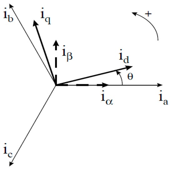
Figure 1. D-Q stationary and synchronous reference frames for three-phase current signals.

These three components have a 120° phase difference and form a rotating current vector over time. By projecting this vector onto a two-dimensional stationary frame, the analysis can be simplified. This process is known as the Clarke transformation and is defined by Equation (1):

$$\left[\begin{array}{c}{\mathrm{i}}_{\mathsf{\alpha }}\\ {\mathrm{i}}_{\mathsf{\beta }}\end{array}\right]={\displaystyle \frac{2}{3}}\left[\begin{array}{ccc}1& \hspace{1em}-{\displaystyle \frac{1}{2}}& \hspace{1em}{\displaystyle \frac{1}{2}}\\ 0& \hspace{1em}{\displaystyle \frac{\sqrt{3}}{2}}& \hspace{1em}-{\displaystyle \frac{\sqrt{3}}{2}}\end{array}\right]\left[\begin{array}{c}{\mathrm{i}}_{\mathrm{a}}\\ {\mathrm{i}}_{\mathrm{b}}\\ {\mathrm{i}}_{\mathrm{c}}\end{array}\right]$$

(1)

Here, ${\mathrm{i}}_{\mathsf{\alpha }}$ represents the component in the fixed a-axis direction, and ${\mathrm{i}}_{\mathsf{\beta }}$ is the orthogonal component in the b-axis direction. The output of the Clarke transformation is useful for visualizing the rotational trajectory of the current vector in a stationary 2D plane. In the event of an unbalanced condition or fault, characteristic asymmetries or distortions in this trajectory often appear.

The (${\mathrm{i}}_{\mathsf{\alpha }},{\mathrm{i}}_{\mathsf{\beta }}$) components obtained through the Clarke transformation are still AC signals that rotate over time. By converting them into a synchronously rotating reference frame aligned with a reference angle θ, these components can be expressed as rectified DC signals under normal operating conditions. This process is called the Park transformation and is defined by Equation (2):

$$\left[\begin{array}{c}{\mathrm{i}}_{\mathrm{d}}\\ {\mathrm{i}}_{\mathrm{q}}\end{array}\right]=\left[\begin{array}{cc}\mathrm{c}\mathrm{o}\mathrm{s}\mathsf{\theta }& \hspace{1em}\mathrm{s}\mathrm{i}\mathrm{n}\mathsf{\theta }\\ -\mathrm{s}\mathrm{i}\mathrm{n}\mathsf{\theta }& \hspace{1em}\mathrm{c}\mathrm{o}\mathrm{s}\mathsf{\theta }\end{array}\right]\left[\begin{array}{c}{\mathrm{i}}_{\mathsf{\alpha }}\\ {\mathrm{i}}_{\mathsf{\beta }}\end{array}\right]$$

(2)

Figure 2 visually illustrates the frequency-domain characteristics of current components under D-Q transformation in a three-phase current source.

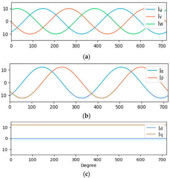
Figure 2. Frequency variation according to D-Q transformation: (a) Three-phase current source, (b) D-Q stationary frame, and (c) D-Q synchronous frame.

Figure 2a shows the original three-phase current waveform during the motor’s operation. Figure 2b displays the current distribution in the stationary reference frame based on Equation (1). Figure 2c presents the frequency characteristics of the current components in the D-Q synchronous reference frame, derived using Equation (2). Under ideal conditions, the Id component in the D-Q frame is expressed as a constant magnitude value without time-domain oscillation, since the frequency components of the three-phase current are rectified with respect to the rotating reference axis.

However, in practical motors, various factors such as internal inductance, copper losses, and iron losses introduce ripple components into the Id signal. These fluctuations become more pronounced under abnormal conditions such as winding short circuits or asymmetric faults.

The Id component derived through the D-Q transformation represents the projection of the three-phase current onto the rotor flux axis. It compresses and integrates physical characteristics such as current magnitude, phase, and spatial distribution into a single reference axis-aligned signal. Thus, ${\mathrm{i}}_{\mathrm{d}}$ serves as a representative component that preserves the overall vector behavior of the three-phase current in a rectified format, acting as a compact information index for the current distribution along a specific axis.

Figure 3 shows the time-domain waveform of the D-axis current (${\mathrm{i}}_{\mathrm{d}}$), obtained from actual measured data, under three conditions: Normal, ITSC, and 4Turn faults.

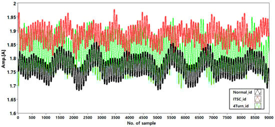
Figure 3. Time-domain waveform of the D-axis current (Id) under three stator conditions: Normal, ITSC, and 4Turn short-circuit faults.

As the number of shorted turns increases, the Id waveform becomes increasingly distorted and exhibits larger amplitude fluctuations.

This behavior clearly demonstrates the sensitivity of Id to stator turn faults, supporting its use as a discriminative diagnostic feature.

In this study, we utilize the one-dimensional time-series data of Id obtained from the D-Q synchronous reference frame to evaluate its temporal variability and sensitivity to faults. This analysis aims to assess the suitability of the Id signal as an input feature for training CNN models.

3.2. Data Measurement and Class Configuration

This experiment was conducted to classify three conditions of a three-phase induction motor: Normal, inter-turn short circuit (ITSC), and a 4Turn short condition in the stator winding.

As shown in Figure 4, the experimental setup includes a 1 HP three-phase induction motor coupled with a dynamometer. The three-phase current measured from the inverter was acquired using Fluke i5s AC current clamps connected to each phase. For data acquisition, an NI USB 9215 with a BNC DAQ device was used.

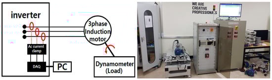
Figure 4. Data measurement setup.

Measurements were taken across a range of speeds, starting from the rated load speed of 1690 rpm up to a partial load speed of 1740 rpm, increasing in 10 rpm increments. At each speed, current data was collected for 30 s.

The sampling frequency was set at 10 kHz, yielding 10,000 samples per second, and the sampling interval was 1 s, in accordance with the DAQ device’s capabilities.

To simulate fault conditions, stator winding faults were intentionally created. As shown in Figure 5, the stator windings of the induction motor were configured to induce an ITSC with 4 turns shorted. Accordingly, the dataset was categorized into three classes: Normal, ITSC, and 4Turn short.

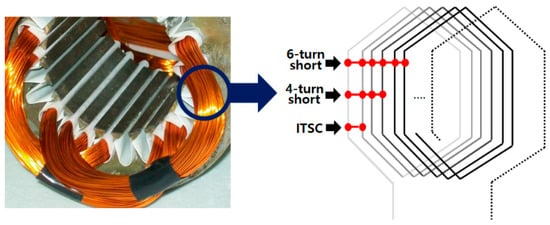
Figure 5. Stator winding short-circuit configuration.

3.3. Raw Data Segmentation

The acquired three-phase current signals were converted into the D-axis component using Equations (1) and (2). From the 10,000 samples per second, the first 1000 samples were discarded to account for signal loss due to motor startup and filtering. Therefore, 9000 samples were used for the actual image conversion.

As shown in Figure 6, the 9000 samples were segmented into chunks of 1024 data points to generate 32 × 32 pixel images. Consequently, 8 image samples were obtained per second.

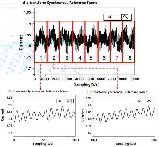
Figure 6. Raw data segmentation.

3.4. Data-to-Image Conversion

This study aims to verify the feasibility of CNN-based fault diagnosis using a single-axis (Id-axis) current by comparing the performance of a CNN diagnosis based on three-phase current image conversion with that based on a Id current. To this end, three widely used methods—three-phase RGB mapping, DWT, and STFT—were each applied using the single-phase (Id) current and compared through image conversion.

3.4.1. Three-Phase RGB Image Construction

To generate CNN input images for fault diagnosis in a three-phase induction motor, the current data from phases A, B, and C were mapped to the RGB channels to form two-dimensional images. This method involves converting the time-series current values into pixel intensities to create an image matrix.

Each phase current signal was normalized to a range of [0, 255] using min–max normalization before being used as CNN input pixel values.

As the normalized data were one-dimensional time-series signals, they were reshaped into a 2D square pixel array for image construction. Specifically, current sequences of a length L = 1024 were sequentially reshaped into a 32 × 32 2D array based on $\sqrt{\mathrm{L}}=32$. Grayscale images were generated for each of the A, B, and C phases.

These grayscale images were then assigned to the RGB channels—Red for phase A, Green for phase B, and Blue for phase C—to construct a single three-channel RGB image.

3.4.2. Three-Phase DWT Image Construction

To generate DWT-based input images, the three-phase current data were first converted from 1D sequences into 2D arrays using sequential reshaping. Each phase signal was then decomposed using a Daubechies 4 (db4) wavelet up to Level 3.

Since the time-series data were aligned horizontally due to the reshape method, the horizontal detail coefficients (cH) were selected from the wavelet-decomposed components. As each cH component output was in grayscale, the grayscale images of phases A, B, and C were mapped to the R, G, and B channels, respectively, to form a three-channel DWT-based RGB image.

3.4.3. Three-Phase STFT Image Construction

STFT is a representative time–frequency analysis technique that divides the time-series signal into fixed-length windows and performs Fourier transforms on each segment, allowing both time and frequency information to be captured.

STFT parameters were configured based on the properties of the raw data used in this study. With a sampling frequency of 10 kHz, the dataset included high-frequency characteristics from localized, rapid fault changes such as 2-turn and 4-turn short faults. Accordingly, a window length of 128 samples (approx. 12.8 ms) was selected, and a time step of 27 samples was used. The frequency resolution was set to 65 frequency bins, enabling an analysis of the 0–5 kHz range at approximately 77 Hz intervals. A Hamming window was applied to reduce the spectral leakage caused by signal discontinuities at boundaries.

The resulting spectrograms for each phase (A, B, C) were grayscale images, which were then assigned to the R, G, and B channels, respectively, to construct STFT-based RGB images.

3.4.4. Id-Linear Image Construction

Since the Id current is provided as a 1D time-series signal, 1024 samples were reshaped into a 32 × 32 2D array using the same sequential reshape method as in the previous experiments. The resulting image was grayscale. As this reshaping method is consistent with the space-filling curve (SFC) linear approach, this method is denoted as Id-Linear in this study.

3.4.5. Id-DWT Image Construction

The sequentially reshaped single-phase data were decomposed using the same method as the three-phase DWT approach. A Daubechies 4 (db4) wavelet was used, with decomposition performed up to Level 3.

Due to the horizontal alignment of the time-series data from the reshape method, the horizontal detail coefficients (cH) at Level 3 were selected, as they best captured the fault characteristics. The extracted cH coefficients were used to construct a grayscale image.

3.4.6. Id-STFT Image Construction

Time–frequency analysis using STFT was applied to the single Id current signal.

The Id current time series consisted of 1024 samples, and the same STFT parameters used for the three-phase STFT were applied: a Hamming window, window length of 128, time step of 27, and 65 frequency bins.

Figure 7 illustrates example images converted using the six methods described above.

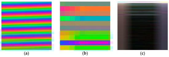
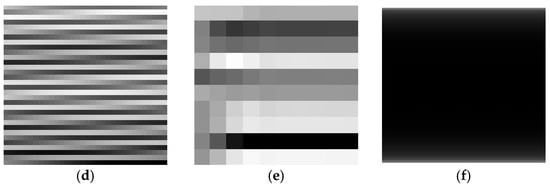
Figure 7. Input image types: (a) 3Phase-RGB, (b) 3Phase-DWT, (c) 3Phase-STFT, (d) Id-Linear, (e) Id-DWT, and (f) Id-STFT.

3.5. Data Splitting and Augmentation

The raw dataset used in this study was collected under six motor speed conditions, ranging from 1690 rpm to 1740 rpm in 10 rpm increments. For each speed segment, 8 images per second were extracted, resulting in 1440 images over a 30 s period. Due to some erroneous measurements, the final number of valid images used in the study was 1424. The dataset was evenly distributed among three fault conditions: Normal, ITSC (inter-turn short circuit), and 4Turn short.

To ensure fair comparison across all methods, the 1424 images were divided as follows: 270 images (approximately 19%) were used as the test set, while the remaining 1154 images were further split into 924 training images and 230 validation images.

To enhance the generalization performance of the deep learning classifier, address data imbalance, and mitigate limitations due to the relatively small training set, a SpecAugment-based data augmentation technique was applied to the training data.

SpecAugment is a data augmentation method specialized for time–frequency images. It applies Time Masking, where random regions along the time axis are masked, and Frequency Masking, where random frequency-axis segments are masked.

In this study, each training image was augmented three times, resulting in a training set four times larger when including the original samples. The same augmentation method was consistently applied to both three-phase current-based images (RGB, DWT, STFT) and single-phase Id current-based images. Figure 8 shows examples of the six image types after applying SpecAugment.

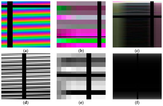
Figure 8. Input images after applying SpecAugment: (a) 3Phase-RGB, (b) 3Phase-DWT, (c) 3Phase-STFT, (d) Id-Linear, (e) Id-DWT, and (f) Id-STFT.

3.6. CNN Configuration

For image classification, a CNN based on the ResNet50 architecture was used, employing a transfer learning framework. The model was configured with include_top = False to remove the default fully connected classification head and replace it with a customized classifier suitable for this study’s objectives.

No pretrained weights were used; instead, all layers were initialized randomly and trained from scratch. The input image size was scaled from 32 × 32 to 224 × 224 × 3 to match the model’s expected dimensions. The architecture was experimentally tuned for stable training, as detailed in Table 1, and the training parameters were set as shown in Table 2.

Table 1. CNN classifier architecture.

Classification	Layer Configuration	Activation Function	Output Dimension	Remark
Feature extractor	ResNET50 (top layer removed; weights = none)		7 × 7 × 2048	Input 224 × 224 × 3
Flatten layer	Flatten		100,352	7 × 7 × 2048 -> 1D
FC layer 1	Dense (512)	ReLU	512	Fully connected layer
	Batch normalization		512	Feature normalization
	Dropout (0.4)		512	Overfitting prevention
FC layer 2	Dense (256)	ReLU	256	Fully connected layer
	Batch normalization		256	Feature normalization
	Dropout (0.3)		256	Overfitting prevention
Output layer	Dense (3)	Softmax	3	No. of classes: 3

Table 2. CNN learning conditions.

Item	Settings
Optimization algorithm	Adam
Initial learning rate	0.0001
Loss function	Categorical cross-entropy
No. of epochs	50
Batch size	32
Callback function	ReduceLROnPlateau, CSVLogger, etc.

4. Experimental Results and Discussion

Figure 9 presents the training and validation accuracy and loss curves for the six different encoding methods.

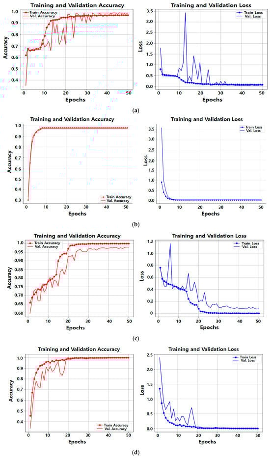
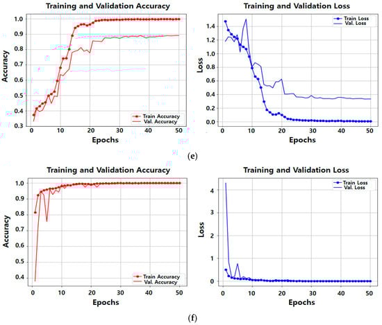
Figure 9. Training and validation accuracy and loss for each of the six encoding methods: (a) 3Phase-RGB; (b) 3Phase-DWT; (c) 3Phase-STFT; (d) Id-Linear; (e) Id-DWT; (f) Id-STFT.

In this study, three strategies were implemented to prevent overfitting:

(1)

Dropout layers (with rates of 0.4 and 0.3) were applied to the fully connected layers to randomly deactivate neurons during training;

(2)

Batch normalization was used to stabilize learning and accelerate convergence;

(3)

ReduceLROnPlateau was employed to automatically decrease the learning rate when the validation loss plateaued.

The effectiveness of these strategies can be observed in Figure 9.

Across all encoding methods, validation accuracy increased in line with training accuracy, and both training and validation loss decreased steadily—indicating that overfitting did not occur during training.

However, in the 3Phase-RGB method, oscillations were observed during the early and middle training stages, and the Id-DWT method exhibited a noticeable gap between training and validation accuracy, suggesting a potential risk of overfitting.

Nevertheless, since all six configurations were trained under identical conditions, and four out of the six methods showed stable and consistent learning curves, the fluctuations in the two cases are likely attributed to sensitivity to the specific input encoding rather than fundamental model instability.

4.1. Training Results

Figure 10 shows the trends in training accuracy and loss for each encoding method across 50 epochs.

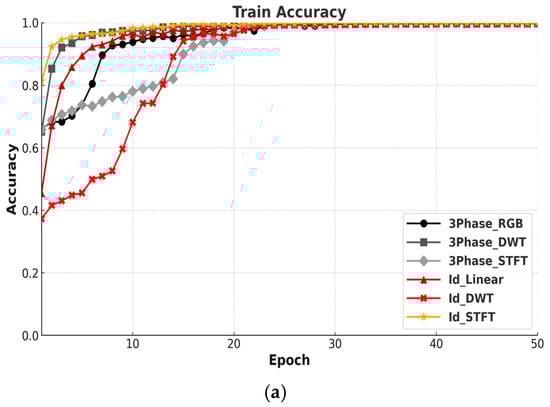
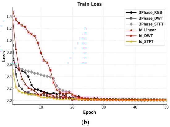
Figure 10. Comparison of training accuracy and loss by encoding method: (a) accuracy; (b) loss.

The training accuracy curves show that the 3Phase-DWT method quickly reaches a high accuracy, demonstrating a strong early performance. Despite using a single-channel input, the Id-STFT method also records the highest training accuracy. In contrast, among the three-phase methods, 3Phase-STFT converges more slowly and attains a lower accuracy. Similarly, within the Id-based methods, Id-DWT converges slowly and yields the lowest training accuracy.

In terms of training loss, both 3Phase-DWT and Id-STFT exhibit a rapid and stable reduction, indicating effective learning. Conversely, 3Phase-STFT and Id-DWT maintain higher loss values and a slower convergence.

These results confirm that all six methods were trained successfully, with no significant oscillations in the learning curves, suggesting an appropriate learning rate. Furthermore, the absence of any increase in training loss indicates that overfitting did not occur.

4.2. Validation Results

Figure 11 compares the validation accuracy and loss to evaluate each encoding method’s generalization performance on unseen data.

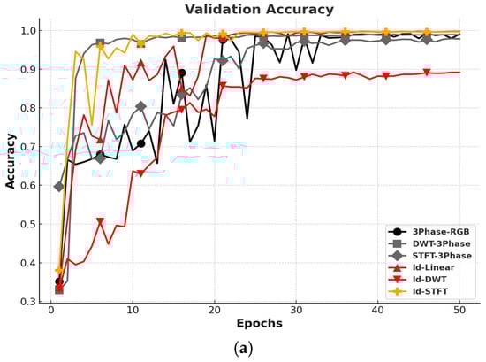
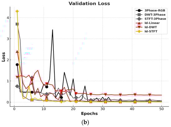
Figure 11. Comparison of validation accuracy and loss by encoding methods: (a) accuracy; (b) loss.

Among the three-phase encoding methods, DWT achieved the highest average validation accuracy of 98.9%, while RGB and STFT recorded similar accuracies of 97.6%. These values were averaged over the final 10 epochs (epochs 41–50).

However, both 3Phase-RGB and 3Phase-STFT exhibited fluctuations in their validation curves during the early and middle training stages. Notably, 3Phase-STFT struggled to converge even in later epochs. In contrast, 3Phase-RGB eventually stabilized and delivered a relatively consistent performance.

For the Id-based encodings, Id-STFT achieved a 99.6% average accuracy, while Id-Linear reached the highest at 99.7%. Conversely, Id-DWT had the lowest performance at 88.8%, indicating that a DWT image derived from a single time series may be insufficient to capture the complexity of fault patterns.

These findings show that single-channel (Id) inputs, when transformed using STFT or linear mapping, can achieve a classification performance and training stability comparable to those of multi-channel, three-phase methods.

Figure 12 compares the best-performing three-phase method (3Phase-DWT) and the best-performing Id-based method (Id-STFT).

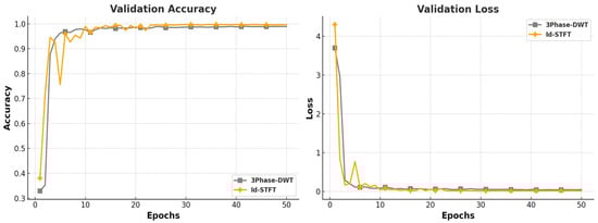
Figure 12. Validation result comparison between 3Phase-DWT and Id-STFT.

Both methods exhibit fast learning and rapid convergence in validation performance, achieving a high accuracy.

This confirms that meaningful feature extraction in the time–frequency domain, as in STFT, enables single time-series inputs to perform comparably to three-channel, three-phase data.

Particularly, Id-STFT benefits from using grayscale input images, which reduces computational and memory demands compared to RGB-based methods—ultimately enabling a faster and more efficient fault diagnosis.

4.3. Test Result

Figure 13 visualizes the confusion matrices for the six encoding methods (RGB, DWT, STFT for 3Phase; linear, DWT, STFT for Id) applied to the test set (270 samples each for ormal, ITSC, and 4Turn), allowing a comparative analysis of models’ prediction accuracy.

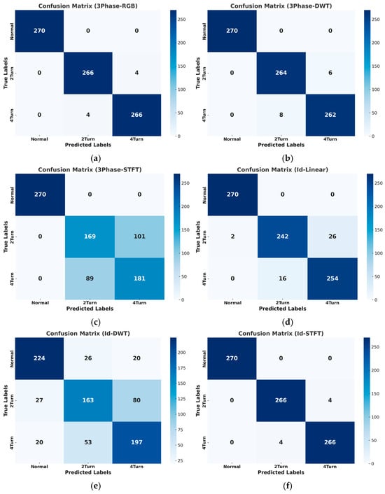
Figure 13. Confusion matrix results for the six encoding methods: (a) 3Phase-RGB; (b) 3Phase-DWT; (c) 3Phase-STFT; (d) Id-Linear; (e) Id-DWT; (f) Id-STFT.

Table 3 presents the test accuracy derived from the confusion matrices in Figure 13. Accuracy was calculated using the formula (TP + TN)/(total number of samples).

Table 3. Test accuracy.

	3Phase -RGB	3Phase -DWT	3Phase- STFT	Id -Linear	Id -DWT	Id -STFT
Test Acc.	99.01%	98.27%	76.56%	94.59%	72.11%	99.01%

Among the three-phase image encoding methods, 3Phase-RGB achieved the highest classification accuracy of 99.01%, correctly predicting 270 Normal, 266 ITSC, and 266 4Turn samples. Similarly, among the single-channel (Id) methods, Id-STFT achieved the same accuracy of 99.01%, demonstrating accurate predictions across all fault types and indicating an effective learning of class boundaries.

In contrast, 3Phase-STFT exhibited significant misclassifications: 101 ITSC samples were misclassified as 4Turn, and 89 4Turn samples were misclassified as ITSC. Among the Id-based methods, Id-DWT showed the poorest performance, with 80 ITSC samples misclassified as 4Turn, and 53 4Turn samples misclassified as ITSC. Additionally, 26 Normal samples were misclassified as ITSC, 20 Normal as 4Turn, 27 ITSC as Normal, and 20 4Turn as Normal—highlighting an overall decline in classification accuracy.

Table 4 presents a quantitative comparison of classification performance in terms of precision, recall, and F1-score for the three fault classes (Normal, ITSC, 4Turn), comparing both 3Phase and Id-based encoding methods.

Table 4. Classification performance comparison based on precision, recall, and F1-score.

Classification	Data	Encoding	Normal	ITSC	4Tum
Precision	3Phase	DWT	100.00%	97.06%	97.76%
		RGB	100.00%	98.52%	98.52%
		STFT	100.00%	65.50%	64.18%
	Id	DWT	82.66%	67.36%	66.33%
		Linear	99.26%	93.80%	90.71%
		STFT	100.00%	98.52%	98.52%
Recall	3Phase	DWT	100.00%	97.78%	97.04%
		RGB	100.00%	98.52%	98.52%
		STFT	100.00%	62.59%	67.04%
	Id	DWT	82.96%	60.37%	72.96%
		Linear	100.00%	89.63%	94.07%
		STFT	100.00%	98.52%	98.52%
F1-Score	3Phase	DWT	100.00%	97.42%	97.40%
		RGB	100.00%	98.52%	98.52%
		STFT	100.00%	64.02%	65.58%
	Id	DWT	82.81%	63.67%	69.49%
		Linear	99.63%	91.67%	92.36%
		STFT	100.00%	98.52%	98.52%

Among the three-phase methods, RGB and DWT demonstrated a strong and consistent diagnostic performance, achieving F1-scores above 97% across all classes. Conversely, 3Phase-STFT showed a significantly lower performance, with F1-scores of 64.02% and 65.58% for ITSC and 4Turn classes, respectively.

Among the Id-based methods, Id-STFT outperformed all the others, achieving precision, recall, and F1-scores above 98.52% for all classes. In contrast, Id-DWT yielded relatively low scores, ranging between 66% and 83%, across all metrics and classes.

In summary, Id-STFT effectively balances computational efficiency—through grayscale input—and a high diagnostic performance, even outperforming RGB-based models in some cases.

4.4. Discussion

Figure 14 presents a comparison of training, validation, and test accuracies for all six encoding methods: 3Phase-RGB, 3Phase-DWT, 3Phase-STFT, Id-Linear, Id-DWT, and Id-STFT.

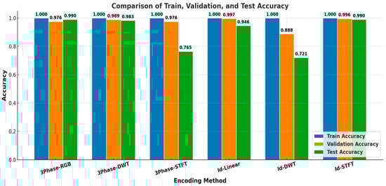
Figure 14. Comparison of training, validation, and test accuracy of the six methods.

Experimental results indicate that 3Phase-RGB and 3Phase-DWT among the three-phase methods, and Id-STFT and Id-Linear among the single time-series methods, demonstrated an overall superior classification performance. Notably, Id-STFT maintained a consistently high accuracy across training and validation phases and matched or surpassed the generalization performance of multi-channel methods—despite using only a single time-series input.

However, despite its high accuracy, 3Phase-RGB exhibited persistent oscillations in validation accuracy during training. As noted in previous studies, the RGB encoding method is sensitive to input noise and simply assigning A, B, and C phases to the R, G, and B channels may inadequately capture meaningful variations in the time–frequency domain. These structural limitations are especially vulnerable to degradation when data augmentation techniques like SpecAugment are applied. Nevertheless, the 3Phase-RGB method showed a gradual convergence in performance toward the latter stages of training, confirming that a certain level of classification accuracy can be achieved. Therefore, while this approach demonstrates the potential for practical use, it also suggests the need for structural improvements in terms of training stability.

Among the three-phase methods, DWT demonstrated the most stable convergence and highest overall performance, with test accuracy closely matching validation accuracy—indicating strong generalization. In contrast, 3Phase-STFT suffered a notable drop in test accuracy, suggesting that the features learned during training did not generalize well to actual fault data. This likely stems from suboptimal image generation due to non-ideal STFT parameters, such as window size and step settings.

For the single time-series approaches, Id-STFT consistently delivered an excellent accuracy and stability across all stages, confirming its effectiveness. In contrast, Id-DWT exhibited unstable and unreliable results, likely due to the loss of critical fault features during the wavelet decomposition process.

Interestingly, Id-Linear, despite its relatively simple encoding structure, achieved an above-average performance. Its computational efficiency and simplicity make it a promising candidate for lightweight model deployment and real-time fault diagnosis systems.

5. Conclusions

This study quantitatively evaluated the diagnostic performance of traditional three-phase (A, B, C) current-based image encoding methods versus a simplified encoding method using only the Id component derived from the D-Q synchronous reference frame. Specifically, the method fixes the Iq component at zero and uses Id as a one-dimensional time-series input to assess whether a single-axis current component can sufficiently retain fault-relevant information without relying on multi-channel data.

Among the three-phase encoding methods, 3Phase-RGB, which maps each phase to the R, G, and B channels, achieved a validation accuracy of 97.6% and a test accuracy of 99%, indicating strong performance. However, oscillations in validation accuracy and loss were observed during the early to mid stages of training, suggesting potential instability in the learning process. Although these effects diminished in later epochs, structural improvements are needed to enhance the model’s stability. In contrast, 3Phase-DWT consistently produced excellent results across all evaluation metrics. Conversely, 3Phase-STFT showed a poor overall performance, likely due to suboptimal window size and step parameter settings for the raw data, indicating the need for further research and refinement.

Among the Id-based encoding methods, Id-STFT demonstrated the highest accuracy, achieving a validation accuracy of 99.6% and a test accuracy of 99%, despite using only a single-channel input. Although grayscale encoding may be perceived as less expressive than RGB, the strong results confirm that it can serve as a fast and effective encoding method. In contrast, Id-DWT exhibited a low overall accuracy, which may be due to a partial loss of fault features during wavelet-based frequency decomposition. The Id-Linear method, despite not involving complex frequency transforms, uses a simple mapping technique to convert time-series data into a 2D image format. It still achieved a strong performance, with a validation accuracy of 99.7% and a test accuracy of 94.6%. Due to its simplicity, this method offers practical advantages for model simplification and real-time diagnostic system deployment. Future work incorporating lightweight neural network models could further expand its applicability.

Overall, this study experimentally verified that encoding methods based on the single-axis Id current obtained through D-Q transformation can perform as well as—or better than—traditional three-phase current-based methods. These findings are attributed to the inherent advantages of the D-Q synchronous frame, including simplified signal structure, elimination of phase imbalance, and reduced sensitivity to noise—all of which positively impact CNNs’ input image quality.

Therefore, this study demonstrates the validity of an alternative encoding method for model simplification and lightweight implementation, showing that a high-performance fault diagnosis is achievable without the need for complex multi-channel inputs.

Furthermore, while the current evaluation was conducted using data from a single testbed under controlled conditions, future work will aim to expand the dataset to include a wider range of fault types and operating scenarios. This will include load disturbances, phase imbalance, and external noise conditions, in order to further assess the generalization capability of the proposed approach in real-world environments.

References

- Ali, U. Towards fault diagnosis in induction motor using fractional Fourier transform. arXiv 2024, arXiv:2412.18227. [Google Scholar] [CrossRef]
- Gubarevych, O.; Gerlici, J.; Kravchenko, O.; Melkonova, I.; Melnyk, O. Use of Park’s vector method for monitoring the rotor condition of an induction motor as a part of the built-in diagnostic system of electric drives of transport. Energies 2023, 16, 5109. [Google Scholar] [CrossRef]
- Enejo, I.S.; Adegboye, B.; Imoru, O.; James, T.O. Fault diagnosis in a three-phase induction motor using enhanced Park vector approach. In Proceedings of the 2022 IEEE Nigeria 4th International Conference on Disruptive Technologies for Sustainable Development (NIGERCON), Lagos, Nigeria, 6–10 June 2022; pp. 1–6. [Google Scholar] [CrossRef]
- Zhang, S.; Wang, R.; Si, Y.; Wang, L. An improved convolutional neural network for three-phase inverter fault diagnosis. IEEE Trans. Instrum. Meas. 2022, 71, 1–15. [Google Scholar] [CrossRef]
- Mohammad-Alikhani, A.; Jamshidpour, E.; Dhale, S.; Akrami, M.; Pardhan, S.; Nahid-Mobarakeh, B. Fault diagnosis of electric motors by a channel-wise regulated CNN and differential of STFT. IEEE Trans. Ind. Appl. 2025, 61, 3066–3077. [Google Scholar] [CrossRef]
- Zhang, B.; Chen, C.; Wang, Y.; Li, J. STFT based CNN for interturn short circuit fault diagnosis of permanent magnet synchronous motor. In Proceedings of the 2024 3rd International Symposium on Semiconductor and Electronic Technology (ISSET), Xi’an, China, 19–21 April 2024; pp. 400–404. [Google Scholar] [CrossRef]
- Xu, M.; Gao, J.; Zhang, Z.; Wang, H. Bearing-fault diagnosis with signal-to-RGB image mapping and multichannel multiscale convolutional neural network. Entropy 2022, 24, 1569. [Google Scholar] [CrossRef]
- Łuczak, D. Machine fault diagnosis through vibration analysis: Time series conversion to grayscale and RGB images for recognition via convolutional neural networks. Energies 2024, 17, 1998. [Google Scholar] [CrossRef]
- Łuczak, D.; Brock, S.; Siembab, K. Fault detection and localisation of a three-phase inverter with permanent magnet synchronous motor load using a convolutional neural network. Actuators 2023, 12, 125. [Google Scholar] [CrossRef]
- Yu, T.; Jiang, Z.; Ren, Z.; Zhou, Y.; Zhang, Y.; Gao, R. A convolutional multisensor fusion fault diagnosis framework based on multidimensional distance matrix for rotating machinery. Struct. Health Monit. 2024. published online. [Google Scholar] [CrossRef]
- Ahmed, H.O.A.; Nandi, A.K. Connected components-based colour image representations of vibrations for a two-stage fault diagnosis of roller bearings using convolutional neural networks. Chin. J. Mech. Eng. 2021, 34, 37. [Google Scholar] [CrossRef]
- Xing, Z.; Liu, Y.; Wang, Q.; Zhao, L.; Chen, Y. Fault diagnosis of rotating parts integrating transfer learning and ConvNeXt model. Sci. Rep. 2025, 15, 190. [Google Scholar] [CrossRef]
- Piedad, E.; Del Rosario, C.A.; Prieto-Araujo, E.; Gomis–Bellmunt, O. Exploring wavelet transformations for deep learning-based machine condition diagnosis. In Proceedings of the 2024 International Conference on Diagnostics in Electrical Engineering (Diagnostika), Pilsen, Czech Republic, 10–12 September 2024; pp. 1–4. [Google Scholar] [CrossRef]
- Le, V.D.; Nguyen, N.B.; Le, Q.C. Deep learning method for fault diagnosis in high voltage transmission lines: A case of the Vietnam 220 kV transmission line. Int. J. Electr. Eng. Inform. 2022, 14, 254–275. [Google Scholar] [CrossRef]
- Paraskevopoulos, D.; Spandonidis, C.; Giannopoulos, F. Hybrid wavelet–CNN fault diagnosis method for ships’ power systems. Signals 2023, 4, 150–166. [Google Scholar] [CrossRef]
- Hsueh, Y.-M.; Ittangihal, V.R.; Wu, W.-B.; Chang, H.-C.; Kuo, C.-C. Fault diagnosis system for induction motors by CNN using empirical wavelet transform. Symmetry 2019, 11, 1212. [Google Scholar] [CrossRef]
- Pietrzak, P.; Wolkiewicz, M. Application of continuous wavelet transform and convolutional neural networks in fault diagnosis of PMSM stator windings. Bull. Pol. Acad. Sci. Tech. Sci. 2024, 72, 150202. [Google Scholar] [CrossRef]
- Fu, G.; Wei, Q.; Yang, Y. Bearing fault diagnosis with parallel CNN and LSTM. Math. Biosci. Eng. 2024, 21, 2385–2406. [Google Scholar] [CrossRef] [PubMed]
- Ni, Y.; Li, S.; Guo, P. Discrete wavelet integrated convolutional residual network for bearing fault diagnosis under noise and variable operating conditions. Sci. Rep. 2025, 15, 16185. [Google Scholar] [CrossRef]
- Saravanan, N.; Ramachandran, K.I. Incipient gear box fault diagnosis using discrete wavelet transform (DWT) for feature extraction and classification using artificial neural network (ANN). Expert. Syst. Appl. 2010, 37, 4168–4181. [Google Scholar] [CrossRef]
- Appiah, M.K.; Danuor, S.K.; Bienibuor, A.K. Performance of continuous wavelet transform over Fourier transform in feature resolutions. Int. J. Geosci. 2024, 15, 87–105. [Google Scholar] [CrossRef]
- Piedad, E.; Mayordo, Z.G.; Prieto-Araujo, E.; Gomis-Bellmunt, O. Deep learning-based machine condition diagnosis using short-time Fourier transformation variants. In Proceedings of the 2024 International Conference on Diagnostics in Electrical Engineering (Diagnostika), Pilsen, Czech Republic, 10–12 September 2024; pp. 1–4. [Google Scholar] [CrossRef]
- Song, X.; Li, Z.; Liu, Y. MVB fault diagnosis based on time-frequency analysis and convolutional neural networks. Sci. Rep. 2025, 15, 5271. [Google Scholar] [CrossRef]
- Ali, U.; Ali, W.; Ramzan, U. An improved fault diagnosis strategy for induction motors using weighted probability ensemble deep learning. arXiv 2024, arXiv:2412.18249. [Google Scholar] [CrossRef]
- Son, T.; Hong, D.; Kim, B. Multi–output classification based on convolutional neural network model for untrained compound fault diagnosis of rotor systems with non–contact sensors. Sensors 2023, 23, 3153. [Google Scholar] [CrossRef]
Disclaimer/Publisher’s Note: The statements, opinions and data contained in all publications are solely those of the individual author(s) and contributor(s) and not of MDPI and/or the editor(s). MDPI and/or the editor(s) disclaim responsibility for any injury to people or property resulting from any ideas, methods, instructions or products referred to in the content. |
© 2025 by the author. Licensee MDPI, Basel, Switzerland. This article is an open access article distributed under the terms and conditions of the Creative Commons Attribution (CC BY) license (https://creativecommons.org/licenses/by/4.0/).