Automatic 3D Reconstruction: Mesh Extraction Based on Gaussian Splatting from Romanesque–Mudéjar Churches

Featured Application

Architectural 3D virtual reconstruction.

Abstract

This research introduces an automated 3D virtual reconstruction system tailored for architectural heritage (AH) applications, contributing to the ongoing paradigm shift from traditional CAD-based workflows to artificial intelligence-driven methodologies. It reviews recent advancements in machine learning and deep learning—particularly neural radiance fields (NeRFs) and its successor, Gaussian splatting (GS)—as state-of-the-art techniques in the domain. The study advocates for replacing point cloud data in heritage building information modeling workflows with image-based inputs, proposing a novel “photo-to-BIM” pipeline. A proof-of-concept system is presented, capable of processing photographs or video footage of ancient ruins—specifically, Romanesque–Mudéjar churches—to automatically generate 3D mesh reconstructions. The system’s performance is assessed using both objective metrics and subjective evaluations of mesh quality. The results confirm the feasibility and promise of image-based reconstruction as a viable alternative to conventional methods. The study successfully developed a system for automated 3D mesh reconstruction of AH from images. It applied GS and Mip-splatting for NeRFs, proving superior in noise reduction for subsequent mesh extraction via surface-aligned Gaussian splatting for efficient 3D mesh reconstruction. This photo-to-mesh pipeline signifies a viable step towards HBIM.

1. Introduction

Digital-based architectural heritage (AH) restoration methods [1], specifically in what is called virtual reconstruction, have gained prominence in the past two decades [2]. This has been mainly due to novel data collection, computer graphics, and computer-aided design (CAD) technologies, and their wide adoption. The last of these is artificial intelligence (AI), which “suggests a turning point that may change in the coming years the way we approach, from a scientific point of view, the question of virtual reconstruction” [3]. In turn, the current AH practice is traversing a paradigm shift from “by hand,” craft-based methods, through 3D modeling and rendering, towards AI-based ones. Central to AH practice, virtual reconstruction is defined as a means of inferring or guessing, based on available information, a building’s possible original state. The latter entails representing a prediction of its original appearance, or its intermediate states, from observation of its existing remains. Here, and this is the main point, “virtual” means that the building is not physically intervened, but it is immaterially invoked via drawing plans, perspectives, isometric views, paintings, or scale model representations [3].

Examples of the aforementioned advancements [4,5,6,7] comprise mainly light detection and ranging (LiDAR) surveying and data capture [8], photogrammetry, videogrammetry [9], virtual reality [10], fractal mesh representation [11], and parametric modeling. These have significantly reduced the difficulty of studying decayed and even disappeared buildings such as Renaissance-era palaces [12], museums [6], and residential buildings [13], including the development of detailed finite element models aimed at the structural assessment of historical constructions at risk of disappearance [14,15]. However, AH’s most recent digital advancement came in the form of building information modeling (BIM), and the later advent of heritage BIM (HBIM), a heritage-specific BIM class system [16]; this means that within the BIM environment, specific classes—or families—are identified that go beyond traditional BIM elements. These recent methods have superseded “traditional” ones due to their further reduced invasiveness in comparison with earlier methods. Roughly speaking, the AH workflow usually works this way: LiDAR technicians, surveyors, art historians, and archaeologists capture data, mainly in the form of point clouds. Then, they submit these data to 3D artists and technicians who reconstruct a detailed digital representation of 3D models. Finally, AH professionals use these as a foundation and support material for their decision-making processes [4].

Benefits aside, non-automated CAD work is still the norm within these practices [10], and significant technical setbacks stem from this kind of 3D acquisition and modeling work. In addition, these conventional methods are usually labor-intensive, time-consuming, and often supported by few and thinly automated processes [2,4,6,13]. Moreover, there have been documented difficulties in establishing precise geometry during mesh reconstruction, often taking significant amounts of time to complete [6]. Furthermore, scan cleaning-related noise problems (i.e., reducing excess points from the usual LiDAR-generated point cloud) and incomplete documentation [7] are commonplace. Last, but more importantly, is their non-reusability, meaning that each building has to be reconstructed from scratch every time a new project begins [17].

In this context, Scan to BIM has emerged in the last decade as a solution “program” to address these issues and automate the whole process. Scan-to-BIM is a process that converts digital point-cloud models obtained through laser scanning into BIM platforms, which analyze the data and incorporate them into a 3D model of the site or building to support development, design, and construction teams [18]. Furthermore, machine learning (ML) is defined as “an aspect of artificial intelligence that competently performs automation in the process of building analytical models that allow machines to adapt independently to new scenarios, enabling software to successfully predict and react to the deployment of scenarios based on past results” [19]; or as a field of study that allows computers to learn autonomously without being explicitly programmed [20]. Deep learning (DL) is defined by [21] as models that can learn representations of data with multiple levels of abstraction and discover structure in large datasets. Even though there have been some partial Scan-to-BIM AI-based successes, no fully automated workflow is yet to be devised [22], meaning that it is plausible for AI to continue filling certain methodological gaps in the fabric of the Scan-to-BIM workflow.

In this scenario, we propose an automatic 3D reconstruction method that provides AH specialists with an ML-based, 3D mesh reconstruction tool that automates the AH 3D modeling step of the general building process, thereby helping to reduce modeling errors, lightening project workloads, shortening completion times, costs and on-site resource expenditures, and facilitating the initial part of the Scan-to-BIM process. This means that the system automates 3D mesh reconstruction of AH from image/video inputs, moving beyond traditional, labor-intensive manual CAD methods. This approach directly reduces modeling errors and lightens project workloads by streamlining the geometric information generation process. Crucially, it replaces conventional, often problematic, point cloud inputs derived from expensive LiDAR or complex photogrammetry with more accessible photographic or video data. This shift intrinsically shortens completion times, lowers costs, and minimizes on-site resource expenditure. By leveraging Gaussian splatting (GS) and its noise-reducing variant, Mip-splatting for radiance field rendering (RFR), followed by surface-aligned Gaussian splatting for efficient 3D mesh reconstruction (SuGaR), the process becomes more efficient, particularly with Mip-splatting’s superior noise reduction. This “photo-to-mesh” pipeline represents a crucial initial step in the Scan-to-BIM process for AH (HBIM), paving the way for AI-driven methodologies. We aim to achieve this by replacing point cloud input with video or photo entries in the Scan-to-BIM process, which we divided into two parts (photo-to-mesh and HBIM class binding), thus outlining a “photo-to-mesh” workflow.

For this specific work, we focused on a “video” or “photo-to-mesh” pipeline for application in the AH virtual reconstruction process, where we used and tested three models in total. The first two, GS [23] and Mip-splatting [24] (a noise-reduction version of GS), both add a photo input step before the point cloud one. Additionally, a third model, SuGaR [25], takes the GS/Mip-splatting output point cloud and reconstructs a textured mesh. This mesh reconstruction step is the one immediately before the HBIM class binding step; we left the latter for future work.

At a broader architectural theory level, we put another brick in the edifice by extending, from BIM to AI [12], a broader question on constructing architectural knowledge through semantic modeling systems and their automation. As claimed, BIM systems “emphasize the use of a semantic construction of the digital model, not only as a means to modeling a building but as a cognitive system” [12]. In other words, our leitmotif question was whether AI, and, more specifically, ML can change our way of thinking about AH. We therefore claim that AI application in AH, at a cognitive level, bridges the gap between “by hand” work and automatic building reconstruction. In turn, this bypasses “manual” CAD modeling and thus changes AH’s internal nature.

Henceforth, this paper is structured in seven sections. The state-of-the-art (SOTA) section briefly describes foundational, previous, and related works. This is followed by a Materials and Methods section that details the datasets used, their pre-processing, framing, the models’ architecture, their tuning, optimization, and validation strategies. Moreover, we present a Results and Evaluation section that explains the experiments conducted and their objective and subjective evaluations, employed for model performance appraisal. In addition, the Discussion section speculates on our experimental results’ overarching implications in relation to Scan-to-HBIM and ML application to AH. The Limitations section outlines the method’s lingering problems and obstacles to better performance and results. Furthermore, a Conclusions section is presented, whose focus is on where automatic 3D reconstruction currently sits within Scan-to-BIM processes. Lastly, Future Work delves into the avenues for further development, the steps considered for an HBIM capstone model, and a possible full pipeline.

2. State of the Art

This section aims to provide an overview of the field of 3D DL, the predecessor of GS and SuGaR, as well as a summary of the research advancements and papers that have been published over the last few years, a timeline whereof is shown in Figure 1. As its name suggests, 3D DL is a field within DL that works with three-dimensional data types and representations. Unlike other fields of computer vision that work with 2D images generally represented as pixel tensors, 3D models have different types of representations, such as point clouds, voxels, polygonal meshes, or neural representations, which open multiple opportunities when working with them. RFR is a Novel View Synthesis, an ML application to the field of computer graphics that takes scene data captured from photos or videos and builds 3D rendered representation models. Neural field rendering (NeRF) [26] had been the historical SOTA RFR incarnation [23].

Due to the scarcity of 3D datasets, most papers have studied the reconstruction of 3D objects from images taken from different angles, measuring the reconstruction error on projections of the object. This means 3D-“constructing” the predicted geometry, rasterizing it, and comparing the output images with the original ones from the same camera angles. Two of the main challenges of 3D DL are, firstly, to find the balance between the amount of input data (images) needed and the detail level of the output 3D model, and, secondly, to reduce model training computational cost, as it is usually very high. Both points must be considered when developing and testing these kinds of AI models.

Historically, 3D DL started with 3D reconstruction from both single-view and multi-view images, such as perspective transformer nets, which is a volumetric scene reconstruction solution based on voxels from single-view images using a projection function to compare 2D images, obtaining SOTA results [27]. Other methods emerged using voxels and polygonal meshes, utilizing the OpenGL renderer [28]. Later, an algorithm for applying gradient descent to polygonal mesh rendering and mesh reconstruction from single-view images was devised, providing SOTA results [29]. NeRF established itself as the SOTA standard in Novel View Synthesis methods by using a multi-layer perceptron (MLP) network as a form of compact and continuous representation of a single 3D scene. From multi-view images, NeRF interpolates the rest of the views of the scene [26]. Around 2020, PyTorch3D [30] began being widely adopted and would later become the standard library for 3D DL. It was created in PyTorch with operators and functions specialized in 3D DL. Furthermore, a model called PolyGen performed 3D reconstruction of polygonal meshes from .obj files using the Transformer architecture [31,32]. In addition, a stream of NeRF-stemming methods emerged, cementing its dominance, such as NeRF in the Wild, which is an evolution of the NeRF model [33]. The first was Instant Neural Graphics Primitives (INGP), a NeRF-like model improved via modifications in gradient computation and the use of hash-grids [34] that attempted to cut NeRF training times, yet did not provide SOTA quality. Then, Neuralangelo [35] was proposed, itself based on INGP, which optimizes training speeds while not achieving SOTA image quality either. Later, DreamFusion was devised, a model that implemented text-to-3D generative capabilities from pre-trained diffusion and NeRF models [36]. Finally, NeRFMeshing [37] emerged, a signed surface approx. network (SSAN) model that, based on the implicit representation of another NeRF model, rendered a 3D polygonal mesh.

Figure 1. Evolution of DL methods for 3D reconstruction from images [25,26,27,28,29,30,32,33,34,35,36,37,38]. Figure created by the authors.

Figure 1. Evolution of DL methods for 3D reconstruction from images [25,26,27,28,29,30,32,33,34,35,36,37,38]. Figure created by the authors.

Until recently, NeRF methods provided the highest visual quality and were considered the SOTA in the field of RFR, most notably Mip-NeRF360 [38], which can take as long as 48 h of training time, its main limitation. This landscape changed when a new model, GS, devised by [23], achieved similar Mip-NeRF360-SOTA quality with training and processing times reduced by a factor of 10. GS was followed in turn by contributions regarding mesh geometry extraction by [25] and which are both used as the basis of our proposed composite system. However, before GS, there had been other fast methods, such as Plenoxels [39] and INGP, identified by [34], that attempted to cut NeRF training times but failed to achieve SOTA quality levels [23,25].

GS uses a NeRF-similar basis, namely the Structure from Motion (SfM) [40] camera calibration, but it then uses its SfM’s sparse point cloud to randomly set the 3D Gaussians. The Gaussians guide an adaptive density control, iterative discriminator algorithm through α-blending, itself a specific adaptation of stochastic gradient descent (SGD) techniques. This combination is used for removing unnecessary Gaussians or adding the necessary ones. Additionally, GS is equipped with a real-time, tile-based rasterization and GPU sorting rendering solution (based on [41]). This is key whereby it achieves similar training speeds as those of the fastest methods, SOTA image quality, and, as they put it, “the first real-time rendering with high quality for novel-view synthesis” [23].

Nevertheless, GS is not without limitations; there were four unaddressed issues for further research [23], namely: (1) artifact reduction in the context of large Gaussians and where the scene is partially occluded; (2) rendering memory use reduction; (3) further speeding up for performance-essential applications (i.e., AH work where less time spent on processing means more intuitive decision-making); and (4) Gaussian-based mesh reconstruction from captured scenes. In [25], two of these avenues for improvement were addressed, namely (1) artifact reduction by using a mesh regularization term and (2) mesh reconstruction. For this, the authors introduced an innovative reconstruction technique that jointly refines both the Gaussians and the mesh by aligning the former with the scene surface and extracting a coarse mesh from it. They achieved this by using signed distance functions (SDF) and then applying Poisson reconstruction (PR) [42] from the Gaussians’ sampled level set points and normals. Finally, this process continues by aligning and binding new Gaussians to the mesh, which iteratively optimizes both Gaussians and the mesh, using the GS original rasterizer.

3. Materials and Methods

In our experiments, a step-by-step methodology was adopted that consists of five subsequent distinct, yet intertwined phases. These phases are as follows: (1) dataset design; (2) pre-processing; (3) model architecture; (4) hyperparameter tuning; and (5) validation. Both GS and Mip-splatting experiments were run using PyTorch with the following hardware: an Intel Core i7-8700 12-core CPU (Intel, Santa Clara, CA, USA) running at 3.70 GHz, 63.9 DDR4 RAM, and one NVIDIA GeForce RTX 2080 Ti graphics card with 11 GB of dedicated VRAM (NVIDIA, Santa Clara, CA, USA).

For this paper, one Romanesque–Mudéjar church in Spain was used as a case study to test whether the workflow works from A to Z. Preliminary investigations with other examples from the same dataset are consistent with the results that are analyzed in this research, since the other examples from the same dataset exhibit similar characteristics, as they belong to the same architectural style. Church No. 01 in our dataset is an existing one called Nuestra Señora de Arbas in Gordaliza del Pino, located 54 km outside of León, Spain; we show its preliminary results in Section 4, specifically of building state 0 (complete building). A training/test split was conducted on the training data, with 158 for training and 23 images for testing, or 87.29% and 12.70%, respectively, as per default recommendations [23] (they used a MipNeRF360-style training/test split). A second GS experiment was run using Mip-splatting [24], an anti-aliasing implementation of GS that reduces point density in its output point cloud, with the same configuration and tuning as for GS, for which we show results in Section 4.

Furthermore, for the dataset’s design and curation, a part of the team, composed of architects and restoration specialists, classified and selected the architectural types, typologies, and style varieties based on historical relevance and technical pertinence regarding which ancient buildings to use as case studies in the dataset, how to classify them, and how to evaluate their state concerning building state, building and component coherence, architectural style, and order. Finally, the entirety of the dataset produced and used in this project was 100% synthetic and manually completed by researchers using SketchUp Pro for modeling and V-Ray NEXT for rendering.

3.1. Dataset Design

The acquisition of “real-world” AH period data poses significant logistical and technical challenges. When trying to gather LiDAR data, some parts are usually occluded from view. In addition, density in its point cloud output format is often impractical for virtual reconstruction tasks, with its point count usually in the billions. This, in turn, produces a significant amount of “outlier” points (or, in the ML language, noise), and processing these in an automated manner is a significant hurdle. A similar type of problem arises when performing photogrammetry to obtain AH building data; occluded points are a common and difficult hindrance due to camera positions and their respective ranges. We also note that both methods, by far the most popular, present similar equipment expertise-related issues, often being extremely expensive and complicated to operate, requiring specialized personnel to manipulate them. Hence, we opted to produce our synthetic dataset to simulate a video capture from a drone or smartphone and simplify the data capture method. The justification for using a synthetic dataset for training, instead of a photographic image set, is thoroughly addressed in our other publications [17]. Finally, our non-invasive strategy of developing synthetic training datasets provides, as a byproduct, the advantage of intervening even less directly in the studied building, overcoming a significant problem in AH processes. Concerning Romanesque–Mudéjar churches, they were chosen as subjects because numerous churches remain in usable states, and there is significant historical documentation available showing them in their original state. We took advantage of this, as it was easier to collect data from the existing or documented buildings and to 3D model them for AI training.

For these reasons, we built a synthetic dataset that comprises 60 Romanesque–Mudéjar style medieval churches, which were 3D-modeled using photographs, surveyed “as-built” plans, sketches, and written descriptions as bases for the modeling of each church. These 3D models were then used to produce rendered images, displaying the building’s materials, light, and shadows against a standard background environment. In turn, these were used to train the GS–SuGaR models, build 3D RFRs, and thereafter extract their respective meshes. To build a systematic dataset, we rendered each church, defining three building states (cf. “snapshots” of the building’s decay process at specific points in time for each church, shown in Figure 2) as follows: building state 0 (complete building); building state 1 (missing roof and cornice); building state 2 (mid-height walls); and counting 180 rendered images for each church. At 32,400 images in total, this dataset is relatively small, but this order of magnitude can be useful if its data framing and processing are adequately implemented, as [17,43] noted. The criterion for selecting the number of images follows the same approach used by [23] in GS, as well as by [38] in Mip–NeRF360, taking every 8th photo for testing, to ensure consistent and meaningful comparisons for the generation of error metrics.

3.2. Pre-Processing

Before model training, the 180 images were downsampled; first, through a Mip–NeRF360-like approach, i.e., each image was downsampled to 1/2, ¼, and 1/8 of its original resolution using COLMAP v3.8 [23,44,45]. Preprocessing takes approximately 1H00 to complete for one church.

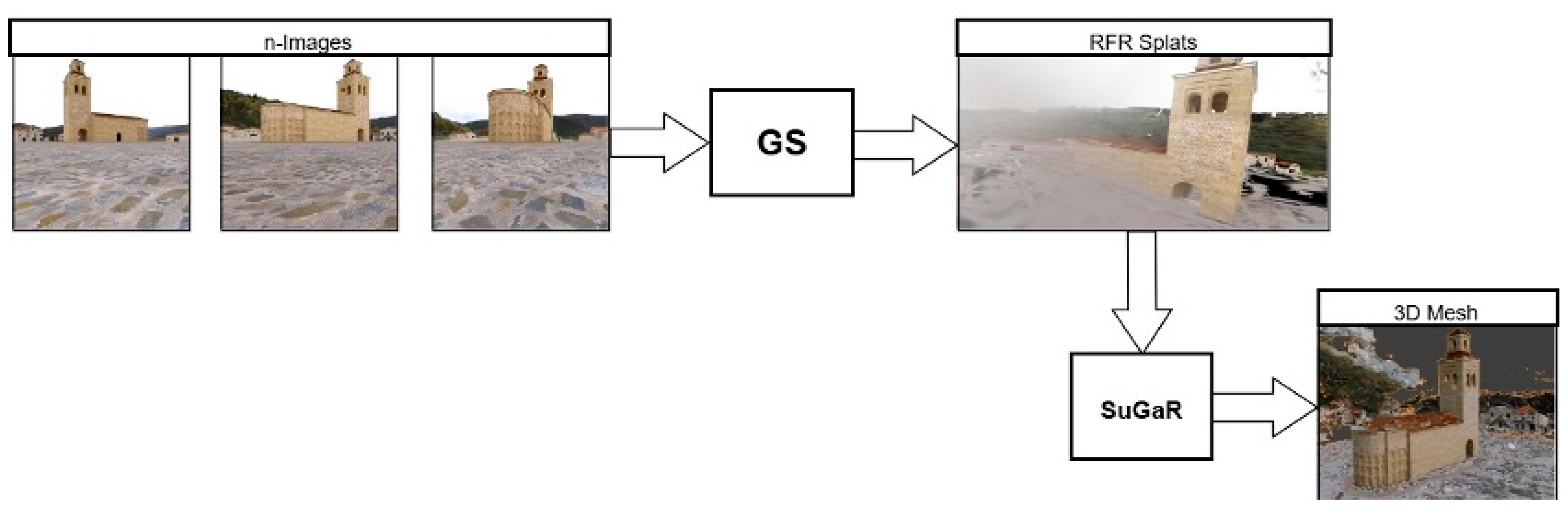
3.3. Model Architecture

The composite system itself is based on two directly related models: (1) GS [23], a novel neural RFR technique that predicts 3D statistical, color-based, spatial strokes, or “splats;” and (2) SuGaR [25], a mesh extraction technique, itself based on GS. The system reconstructs 3D RFR and textured mesh geometry using 180 sequenced, panoramic church images as inputs, and outputs one 3D mesh model of the said church. These take care of image rasterization, RFR, and mesh extraction (in this order). We first break down the rasterization, RFR, and mesh extraction steps, and then present the implementation diagram.

The GS model begins the general process by using a sparse point cloud generated via SfM that places the 3D Gaussians defined by position, covariance matrix, and opacity α. This produces a compact representation of a 3D scene, using spherical harmonics to gauge the directions of the Gaussian splats [23,24]. Then, the algorithm builds a 3D RFR representation by a series of optimization steps: position, covariance, α-blend, SH, all interspersed with adaptive control of Gaussian density [23].

As a reminder of the basics of GS and SuGaR processes, we outline a brief overview of their formalizations for training RFR and mesh extraction. In a typical neural point-based rendering approach, each color of a given pixel is computed by blending the N-ordered points overlapping a given pixel, where ref. [23] used as their starting point the following equation:

$$C=\sum _{i\in N}{c}_i{\alpha }_i\prod _{j=1}^{i-1}\left(1-{\alpha }_j\right)$$

(1)

Here, c_i is the color of each point and α_i is given by evaluating a 2D Gaussian with covariance Σ multiplied by a learned per-point opacity [46]. Plus, they formalized the function for a single Gaussian G, centered at point μ (mean), which is then multiplied by α in the blending process, as follows:

$$G\left(\mathrm{x}\right)=e^{-{\displaystyle \frac{1}{2}}{\displaystyle {\left(x\right)}^T}{\sum }^{-1}{\displaystyle \left(x\right)}}$$

(2)

Furthermore, they defined a scaling matrix S and a rotation matrix R to find the corresponding covariance matrix Σ (cf. a world space) that is used to place the 3D Gaussians [47]:

$$\mathsf{\Sigma }={RSS}^T{R}^T,$$

(3)

where the covariance matrix Σ of a 3D Gaussian is equivalent to describing an ellipsoid. For more details, see [23].

After this step, the SuGaR method takes the Gaussians and, using a loss term, enforces 3D Gaussian and scene–surface alignment during the GS optimization process. This model exploits this alignment for high-detail mesh extraction from Gaussians using signed distance functions. Then, a refinement process that optimizes both mesh and 3D Gaussians on the mesh’s surface is set in motion, using GS’s rendering operation and producing an editable mesh through Poisson reconstruction (PR) [25,42] as output. In their original paper, the SuGaR authors defined their “ideal” SDF associated with a density function $d$, in the case that $d=\overline{d}$; where $p$ is a sampled point, f is its SDF, and $d$ is its density. Their formalization of an ideal function $\mathrm{f}\left(\mathrm{p}\right)$ is as follows:

$$\mathrm{f}\left(\mathrm{p}\right)=\pm s_{g*}\sqrt{-2}\mathit{log}\left(d\left(p\right)\right)$$

(4)

Its approximation, $\overline{f}\left(p\right)$, is as follows:

$$\overline{f}\left(\mathrm{p}\right)=\pm s_{g*}\sqrt{-2}\mathit{log}\left(\overline{d}\left(p\right)\right)$$

(5)

Using these formulas, they rendered depth maps of the Gaussians, and then sampled points $p$ in each viewpoint, each according to the distribution of the Gaussians, where $\overline{f}\left(p\right)$ is the 3D distance between $p$ and the intersection of the line of sight for $p$ and the given depth map. They then applied a regularization term $R$ to compute the latter:

$$R={\displaystyle \frac{1}{\left|P\right|}}\sum _{\mathrm{p}\in \mathrm{P}}\left|\overline{f}\left(\mathrm{p}\right)-f\left(\mathrm{p}\right)\right|$$

(6)

This process works by sampling 3D points $p$ and summing up the differences between the ideal SDF $\mathrm{f}\left(\mathrm{p}\right)$ and an approximate $\overline{f}\left(\mathrm{p}\right)$ of the SDF of the surface generated by the current Gaussians at these given points, where $P$ is the set of sampled points [25]. Please refer to both of their original papers for more details.

From a more practical perspective, a unified modeling language (UML) diagram is given in Figure 3, with human intervention points marked along the workflow.

3.4. Hyperparameter Tuning

After preprocessing, the training dataset is introduced into the GS model until it finds a mapping between both the original input images and the preprocessed ones. This way, the discriminator evaluates if the image belongs to the original dataset and predicts X, Y, Z coordinates, spherical harmonics, and other model parameters. Experimentally, direct training needed 00H22 for GS and 2H00+ for SuGaR, depending on the 3D model’s building state, mesh density, and polygon number. After experimenting with several hyperparameter value combinations and obtaining unsatisfactory results, we settled for the same configuration as both [23,25]. These were limited to the X, Y, Z coordinates and position learning rates, an SGD iteration-based optimization, a sigmoid activation function for α to obtain smooth gradients for the Gaussians, an exponential activation function for the covariance scale set during the GS step, and, lastly, a regularization term introduced in the SuGaR step, albeit the latter has some specificities; e.g., in the SuGaR process, for one optimization-rendering run, up to 7000 iterations, there is no regularization term (loss term, in this case). After that, 2000 iterations are carried out using an entropy loss term, and then, at 9000 iterations, 6000 more iterations are run using the regularization term $R$, outlined in Section 3.3 [25]. These are the only algorithmic hyperparameters tuned in the whole process.

3.5. Validation

GS and SuGaR both use strictly ML techniques that do not train in the same training/validation/test cycle as the GANs [48] or the attention-based, Transformer [31] architectures used in DL methods. Moreover, the models’ final outputs are .ply and .obj files, which are Poisson-reconstructed using GS predicted coordinates, spherical harmonics, and α-blend color opacity, scale, and rotation derived from videos or sequenced photo frames. Therefore, no prompting or any other type of after-training input is required to generate 3D geometry: the input and training data are the same. This means that there is no validation set to evaluate the model directly. In this context, we used a train/test split for model performance to be evaluated via objective metrics, post-processing. We also carried out a subjective results evaluation. The latter is through practical, hands-on 3D model output inspection by the architecture team using Blender 4.0.

4. Results and Evaluation

We carried out two experiments, using both the original GS implementation and Mip-splatting by [24] (a depth field-optimized version of GS), with temple 01, building state 0 from the Romanesque–Mudéjar churches dataset. We successfully performed RFR using both models on the same data, meaning that an RFR model was generated from 180 2D photographs in each experiment, but with performance differences. We then ran SuGaR using both of their .ply point clouds and selected one of the two based on their suitability for the SuGaR mesh extraction step. These processes are shown in Figure 4.

In experiment 1, we used the original GS implementation successfully but with some setbacks. This specific implementation, being designed without anti-aliasing or culling mechanisms, generated noise saturation problems with consequences for the next step (SuGaR), which in turn generated excess polygons in the final output mesh. This compels the human operator to “cleanup” the point cloud, having to delete excess points and polygons at the end of the whole process. Although this is not a handicapping procedure (it takes approximately 5 min to accomplish), if done with a high quantity of meshes to process, it can become a hindrance. This issue also keeps a niche problem open concerning GS: reducing point cloud density (i.e., noise).

In experiment 2, we finally settled on using the Mip-splatting output point cloud to generate the subsequent SuGaR output meshes shown in all the figures hereafter in this article. We used the latter model to reduce the excess points in the resulting point cloud compared to the original GS.

For the SuGaR step, although we obtained the desired 3D textured mesh geometry, we did so with less satisfying results. Even though we used an alias-free version of GS (i.e., Mip-splatting) that reduces excess point count in the previous step, the resulting mesh still presented some, albeit less than GS, excess noise. Nevertheless, point cloud since “cleanliness” was less of an issue in experiment 2, we proceeded with Mip-splatting’s point cloud to “weave” the Poisson Reconstruction to build the mesh (Figure 5).

4.1. Objective Evaluation

Our GS, Romanesque–Mudéjar, in experiment 1, obtained the following scores in SSIM = 0.705, PSNR = 22.61, and LPIPS = 0.371 using GS’s original implementation with no anti-aliasing. While these prices are lower than the ones obtained in the GS original paper, they are still relatively close to the mark, even outdoing Plenoxels [39] and equaling INGP-Base [34] on LPIPS (

Table 1. Objective metrics for evaluating and comparing the GS, Mip-splatting, and SuGaR Romanesque–Mudéjar performances with other Mip-NeRF360 dataset SOTA performances in [23]. Results marked with (†) were obtained in our experiments; all others have been directly transcribed from their original papers.

Romanesque–Mudejar Dataset
Method/Metric	SSIM ↑	PSNR ↑	LPIPS ↓	Train	FPS	Mem
GS Mudéjar 30 K	0.705 †	22.61 †	0.371 †	0 h 21 min 31 s †	-	51.8 MB †
Mip-splatting Mudéjar/30 K	0.665 †	20.66 †	0.335 †	0 h 22 min 00 s †	-	103.9 MB †
SuGaR Mudéjar/30 K	0.482 †	9.88 †	0.630 †	2 h 01 min 15 s †	-	146.8 MB †
Mip-NeRF360 dataset
Plenoxels	0.626	23.08	0.463	0 h 25 min 49 s	6.79	2.1 GB
INGP-Base	0.671	25.30	0.371	0 h 05 min 37 s	11.7	13 MB
INGP-Big	0.699	25.59	0.331	0 h 07 min 30 s	9.4	348 MB
M-NeRF360	0.792	27.69	0.237	48 h 10 min 50 s	0.06	8.6 MB
GS-Kerbl/7 K	0.770	25.60	0.279	0 h 06 min 25 s	160	523 MB
GS-Kerbl/30 K	0.815	27.21	0.214	0 h 41 min 33 s	134	734 MB

The arrows (↑, ↓) indicate the direction in which the proposed indicator shows a positive outcome. The SSIM range, which measures the similarity between two images, spans from 0 to 1, with 1 indicating maximum similarity. PSNR reflects the compression level of the reconstructed image compared to the original, where higher values denote better performance. LPIPS also measures image similarity on a scale from 0 to 1, using a different method than SSIM. Unlike SSIM, in LPIPS a value of 0 indicates the highest similarity. Data compiled by the authors, based on [23].

). Granted, these results are from different datasets, but LPIPS is still the most important metric concerning image analysis. In experiment 2, running the same dataset on the Mip-splatting implementation issued the following scores: SSIM = 0.665, PSNR = 20.66, and LPIPS = 0.335. These are slightly lower than the ones from the original GS model (Table 1), but it also performed better on LPIPS than both Plenoxels and INGP-Base. Furthermore, .obj mesh file verification confirmed that it is the better choice. For the SuGaR step, metrics yielded these values: SSIM = 0.483, PSNR = 9.879, and LPIPS = 0.630. These scores can be interpreted as a step in the right direction in terms of image rasterization evaluation, but are still insufficient for mesh objects, unlike other, more suitable metrics such as point accuracy % (PA) and point precision % (PP), which are intended to be used in future experiments.

In

Table 2. Objective metrics for evaluating and comparing the SuGaR Romanesque–Mudéjar performances with other Mip-NeRF360 dataset SOTA performances only on outdoor scenes in [25]. Results marked with (†) were obtained in our experiments; all others have been directly transcribed from their original papers.

No Mesh Extraction Method (Except SuGaR)
Romanesque–Mudéjar dataset
Method/metric	SSIM ↑	PSNR ↑	LPIPS ↓
SuGaR Romanesque–Mudejar/15 K	9.88 †	0.483 †	0.630 †
Mip-NeRF360 dataset
Plenoxels	22.02	0.542	0.465
INGP-Base	23.47	0.571	0.416
INGP-Big	23.57	0.602	0.375
Mip-NeRF360	25.79	0.746	0.247
3DGS	26.40	0.805	0.173
SuGaR [25]/15 K	24.40	0.699	0.301
With the mesh extraction method
Romanesque–Mudéjar dataset
Method/metric	SSIM ↑	PSNR ↑	LPIPS ↓
SuGaR Romanesque–Mudejar/15 K	9.88 †	0.483 †	0.630 †
Mip NeRF360 dataset
Mobile NeRF	21.95	0.470	0.470
NeRFMeshing	22.23	-	-
BakedSDF	22.47	0.585	0.349
SuGaR [25]/2 K	22.97	0.648	0.360
SuGaR [25]/7 K	24.16	0.691	0.313
SuGaR [25]/15 K	24.40	0.699	0.301

The explanation of the arrows direction (↑, ↓) is the same as in Table 1. Data compiled by the authors, based on [25].

, we show a comparative evaluation between the SuGaR method’s application to our Romanesque–Mudéjar dataset and other NeRF-based RFR and mesh extraction or reconstruction methods, specifically on outdoor scenes. These are Mobile-NeRF [49]; NeRFMeshing [37], and BakedSDF [50], as ref. [25] did in their original paper. As we can see, when used for RFR on the original Mip-NeRF dataset, SuGaR comes in second only to [23] GS on all metrics. When compared with other popular mesh extraction methods, as seen lower in

Table 3. Objective evaluation metrics comparing GS, Mip-splatting and SuGaR only on outdoor scenes using our own Romanesque–Mudéjar datasets. Averages are shown to evaluate overall performance.

Method/Metric	SSIM ↑	PSNR ↑	LPIPS ↓	Train
GS/30 K	0.705	22.610	0.371	0 h 21 min 31 s
Mip-splatting/30 K	0.665	20.660	0.335	0 h 22 min 00 s
SuGaR/15 K	0.482	9.876	0.630	2 h 01 min 15 s
Average (all methods used)	0.618	17.716	0.445	2 h 22 min 23 s

The explanation of the arrows direction (↑, ↓) is the same as in Table 1. Data compiled by the authors.

, it comes in at the top on all metrics. However, when applied to our Romanesque–Mudéjar dataset, it scores last on PSNR and LPIPS but surpasses Mobile-NeRF on SSIM, which highlights that it is a viable method for outdoor 3D reconstruction. However, its PSNR score highlights that the valid signal and noise are hard to distinguish and points towards the still lingering excess points in the Mip-splatting output. Training times and memory usage were not evaluated in mesh extraction metrics.

Taking averages into account, our use of Mip-splatting and SuGaR together overtakes Mobile-NeRF on both SSIM and LPIPS while remaining significantly lower on PSNR. Because of this, it seems to be a viable solution for our “photo-to-mesh” pipeline and a significant step towards a solution to the Scan-to-HBIM problem. We decided to keep Mip-splatting even though it scores lower than GS because it reduces noise significantly, and this contributes to a more efficient point cloud-to-mesh process.

4.2. Subjective Evaluation

This aspect of our model evaluation was carried out by looking directly into the .ply and .obj output files and manually checking for excess points, noise, and imperfections by 3D modeling experts (Figure 6). We established the Luma Labs Capture web app’s implementation of GS and their mesh extraction algorithm [51] as a baseline for quality control by comparison with our locally implemented GS and Mip-splatting-SuGaR composite system instances. Inspecting both Luma Labs GS capture web app’s results and our own using Mip-splatting and SuGaR in experiment 2, we can see that holes are observed around roughly the same rooftop area in both cases (Figure 7). This points towards a shortcoming in our dataset, meaning that it only comprises images at a human observer’s height; thus, there are no images shot from high altitude, such as bird’s-eye views. This, in turn, leads us to believe that vision information is getting lost, such as points around the rooftop.

Furthermore, in agreement with our SuGaR step’s PSNR being significantly lower, we can see that the “real” 3D points and Gaussians get mixed in with the noise (i.e., outlier points, excess points) even when using Mip-splatting’s anti-aliasing method. This points to a render quality issue, and it is not observed in Luma Lab’s Capture web app results. Luma Labs solved the point cloud noise reduction problem through what seems to be post-processing noise reduction techniques. Since their codebase is closed, we are limited in speculating about their post-GS processing techniques.

The Automatic 3D Reconstruction evaluation criteria can be summarized as follows (

Table 4. Automatic 3D Reconstruction Evaluation Criteria.

Element	Description	Quantity
Objectives	3D reconstruction from images	N/A
Architecture type	Stochastic gradient descent + k-nearest neighbors	2 architecture types
Model type	GS + SuGaR	2 models
Building dataset	60 Romanesque–Mudéjar temples	32,400 synthetic images
Input (direct training)	Ruin or complete images	180 images or one 360° video for the building
Output	Reconstructed 3D Mesh	1 3D-textured mesh model
Techniques	Gaussian rasterization + Anti-aliasing + Poisson reconstruction	3 techniques
Training time	Training time without pre-processing	GS = 00H22m; SuGaR = 2H00m
Limitations	No BIM classes output	1,000,000+ pts.

N/A: Not Applicable. Data compiled by the authors.

). The study focuses on 3D reconstruction from images using a combination of GS and SuGaR models, trained through stochastic gradient descent and k-nearest neighbors. It uses a dataset of 60 Romanesque–Mudéjar temples, with over 32,000 synthetic images. Input data includes either 180 images or a 360° video per building. The output is a single textured 3D mesh. Techniques applied include Gaussian rasterization, anti-aliasing, and Poisson reconstruction. Training times vary, with GS requiring 22 min and SuGaR around 2 h. A key limitation is the absence of BIM class outputs, despite processing over one million points.

5. Discussion

Automatic 3D reconstruction’s implications in the ML application to AH practice concern two main aspects: training and dataset.

Training: Previous ARQGAN 1.0 and 2.0 models reconstruct 2D church images, and Mesh Extraction Based on Gaussian splatting from Romanesque–Mudéjar Churches takes said images and reconstructs a 3D RFR model, from which it extracts a geometric mesh from. Coupled together, this is a significant step towards a full Scan-to-HBIM pipeline because it is the step before the element segmentation and IFC-BIM class-binding one. Extending the IFC class system to encompass AH assets as proposed by [52] will render this complete process possible.

Training dataset: We introduced a dataset composed of 60 Romanesque–Mudéjar-style churches in total, both complete and with missing elements, and all the data used therein is photo-based. Other researchers can use our dataset to train their DL or ML models with it. There is no LIDAR or Laser Scanning involved in this process.

6. Limitations

Despite promising results, our models remain somewhat arcane, hermetic, and require ML and DL expertise to be implemented in an actual AH workflow. It is thus necessary that this methodology be simplified for practical use in the field. Luma Labs provides a web app that fills this last gap; nonetheless, its customization possibilities for specific needs are limited, and it presents similar challenges to our implementation concerning missing rooftop points when used with our dataset. This, therefore, remains an open software engineering question.

Edge and geometric culling are another avenue for improvement as it can help reduce excess meshes, outlier points, and artifacts present in both our GS and Mip-splatting resulting point, which is a significant setback. Also, even if these are already significantly reduced by using Mip-splatting as a point cloud generator, post-processing is needed to further reduce noisy output in the Mip-splatting step.

A further limitation is the quantity of photos required by both GS and Mip-splatting to produce the desired RFR outputs in both our experiments. We empirically determined the lower bound at 150 sequenced, high panoramic images, for it to be able to surpass the pre-processing filter and predict sufficiently accurate point coordinates and thus produce more satisfying results.

7. Conclusions

The automated 3D reconstruction system proposed in this study significantly advances AH practices by shifting from non-automated, scanning-based virtual reconstruction to AI-driven methodologies, a core contribution. A primary strength lies in its novel “photo-to-BIM” pipeline, which replaces conventional LiDAR-generated point cloud inputs with more accessible video and photographic data that can be captured by ubiquitous devices like smartphones or drones, thereby mitigating issues of high cost, complex operation, and significant noise inherent in traditional methods. This approach integrates SOTA ML models: GS and its noise-reducing variant Mip-splatting for RFR, followed by SuGaR for efficient textured mesh extraction. The research specifically highlights Mip-splatting’s superior capability in reducing excess points or noise compared to the original GS, which is crucial for a cleaner subsequent point cloud-to-mesh process, even though some noise persisted. Furthermore, the combined use of Mip-splatting and SuGaR demonstrates viability for outdoor 3D reconstruction of AH, outperforming certain other methods in specific metrics. Another significant strength is the creation of a valuable, reusable synthetic dataset of 60 Romanesque–Mudéjar churches, comprising 32,400 render images, which supports non-invasive research and model training while overcoming challenges associated with real-world data acquisition and direct intervention. By automating geometric information generation and bypassing manual CAD modeling, the system lightens professionals’ cognitive load, reduces modeling errors, shortens completion times, lowers costs, and minimizes on-site resource expenditure. This comprehensive approach thus represents a crucial initial step towards a full Scan-to-BIM/HBIM pipeline for AH, bridging the gap between human-driven CAD and AI-automated virtual reconstruction.

8. Future Work

There are several avenues for improvement in our roadmap. Firstly, we are considering the future development of a capstone model that performs 3D semantic segmentation and IFC class binding to close our envisioned AH “photo-to-3D mesh with IFC classes” pipeline. Bypassing the point cloud capture bottleneck in Scan-to-HBIM, this would be usable for heritage BIM architectural representation, established as the AEC industry standard. This time around, using the complete dataset of 60 Romanesque–Mudéjar-style Spanish churches as subjects.

Secondly, point cloud noise may be overcome by implementing post-processing culling techniques after GS and before SuGaR; this is another consideration for improvement concerning this methodology’s practical implementation and use. Furthermore, we are testing newer models, such as few-shot GS, that can probably help lower the photo count required for RFR [53]. Thirdly, we are also currently expanding the render view angles in the dataset to include bird’s-eye aerial perspectives, which we suspect are causing some of the holes seen in the resulting meshes. Finally, another exciting avenue for real-world application is the development of an app that allows restoration, archeological, and AH experts in general to use these models in their daily work without computational expert programmer intervention. This will allow more customization than offered in current online implementations and overcome Luma Lab’s (and our experiments) missing roof points issues.

It is also possible to expand the case studies to other historical typologies—of various historical styles—which, from our perspective, display a series of common patterns that are likely to form clusters.

References

1. Jokilehto, J. Definition of Cultural Heritage: References to Documents in History; ICCROM Working Group ‘Heritage and Society’: Rome, Italy, 2005. [Google Scholar]
2. Berndt, E.; Carlos, J. Cultural Heritage in the Mature Era of Computer Graphics. IEEE Comput. Grap. Appl. 2000, 20, 36–37. [Google Scholar] [CrossRef]
3. Delgado-Martos, E.; Carlevaris, L.; Intra Sidola, G.; Pesqueira-Calvo, C.; Nogales, A.; Maitín Álvarez, A.M.; García Tejedor, Á.J. Automatic Virtual Reconstruction of Historic Buildings Through Deep Learning. A Critical Analysis of a Paradigm Shift. In Beyond Digital Representation; Digital Innovations in Architecture, Engineering and Construction; Springer: Cham, Switzerland, 2023; pp. 415–426. ISBN 978-3-031-36154-8. [Google Scholar]
4. Matini, M.R.; Ono, K. Accuracy Verification of Manual 3D CG Reconstruction: Case Study of Destroyed Architectural Heritage, Bam Citadel. In Digital Heritage; Ioannides, M., Fellner, D., Georgopoulos, A., Hadjimitsis, D.G., Eds.; Lecture Notes in Computer Science; Springer: Berlin/Heidelberg, Germany, 2010; Volume 6436, pp. 432–440. ISBN 978-3-642-16872-7. [Google Scholar]
5. Kersten, T.P.; Lindstaedt, M. Automatic 3D Object Reconstruction from Multiple Images for Architectural, Cultural Heritage and Archaeological Applications Using Open-Source Software and Web Services. Photogramm. Fernerkund. Geoinf. 2012, 2012, 727–740. [Google Scholar] [CrossRef]
6. Autran, C.; Guena, F. 3D Reconstruction of a Disappeared Museum. In Proceedings of the 2014 International Conference on Virtual Systems & Multimedia (VSMM), Hong Kong, China, 9–12 December 2014; IEEE: Piscataway, NJ, USA, 2015; pp. 6–11. [Google Scholar]
7. Autran, C.; Guena, F. 3D Reconstruction for Museums and Scattered Collections Applied Research for the Alexandre Lenoir’s Museum of French Monument. In Proceedings of the 2015 Digital Heritage, Granada, Spain, 28 September–2 October 2015; IEEE: Piscataway, NJ, USA, 2016; pp. 47–50. [Google Scholar]
8. Wang, L.; Chu, C.H. 3D Building Reconstruction from LiDAR Data. In Proceedings of the 2009 IEEE International Conference on Systems, Man and Cybernetics, San Antonio, TX, USA, 11–14 October 2009; IEEE: Piscataway, NJ, USA, 2009; pp. 3054–3059. [Google Scholar]
9. Torresani, A.; Remondino, F. Videogrammetry vs Photogrammetry for Heritage 3D Reconstruction. Int. Arch. Photogramm. Remote Sens. Spat. Inf. Sci. 2019, XLII-2/W15, 1157–1162. [Google Scholar] [CrossRef]
10. Bevilacqua, M.G.; Russo, M.; Giordano, A.; Spallone, R. 3D Reconstruction, Digital Twinning, and Virtual Reality: Architectural Heritage Applications. In Proceedings of the 2022 IEEE Conference on Virtual Reality and 3D User Interfaces Abstracts and Workshops (VRW), Christchurch, New Zealand, 12–16 March 2022; IEEE: Piscataway, NJ, USA, 2022; pp. 92–96. [Google Scholar]
11. Peta, K.; Stemp, W.J.; Stocking, T.; Chen, R.; Love, G.; Gleason, M.A.; Houk, B.A.; Brown, C.A. Multiscale Geometric Characterization and Discrimination of Dermatoglyphs (Fingerprints) on Hardened Clay—A Novel Archaeological Application of the GelSight Max. Materials 2025, 18, 2939. [Google Scholar] [CrossRef]
12. Apollonio, F.I.; Gaiani, M.; Sun, Z. 3D Modeling and Data Enrichment in Digital Reconstruction of Architectural Heritage. Int. Arch. Photogramm. Remote Sens. Spat. Inf. Sci. 2013, XL-5/W2, 43–48. [Google Scholar] [CrossRef]
13. Campi, M.; Di Luggo, A.; Scandurra, S. 3D Modeling for the Knowledge of Architectural Heritage and Virtual Reconstruction of Its Historical Memory. Int. Arch. Photogramm. Remote Sens. Spat. Inf. Sci. 2017, XLII-2/W3, 133–139. [Google Scholar] [CrossRef]
14. Valente, M.; Brandonisio, G.; Milani, G.; Luca, A.D. Seismic Response Evaluation of Ten Tuff Masonry Churches with Basilica Plan through Advanced Numerical Simulations. Int. J. Mason. Res. Innov. 2020, 5, 1–46. [Google Scholar] [CrossRef]
15. Valente, M. Earthquake Response and Damage Patterns Assessment of Two Historical Masonry Churches with Bell Tower. Eng. Fail. Anal. 2023, 151, 107418. [Google Scholar] [CrossRef]
16. Murphy, M.; McGovern, E.; Pavia, S. Historic Building Information Modelling (HBIM). Struct. Surv. 2009, 27, 311–327. [Google Scholar] [CrossRef]
17. Nogales, A.; Delgado-Martos, E.; Melchor, Á.; García-Tejedor, Á.J. ARQGAN: An Evaluation of Generative Adversarial Network Approaches for Automatic Virtual Inpainting Restoration of Greek Temples. Expert Syst. Appl. 2021, 180, 115092. [Google Scholar] [CrossRef]
18. Adekunle, S.A.; Aigbavboa, C.; Ejohwomu, O.A. Scan to BIM: A Systematic Literature Review Network Analysis. IOP Conf. Ser. Mater. Sci. Eng. 2022, 1218, 012057. [Google Scholar] [CrossRef]
19. França, R.P.; Borges Monteiro, A.C.; Arthur, R.; Iano, Y. An Overview of Deep Learning in Big Data, Image, and Signal Processing in the Modern Digital Age. In Trends in Deep Learning Methodologies; Elsevier: Amsterdam, The Netherlands, 2021; pp. 63–87. ISBN 978-0-12-822226-3. [Google Scholar]
20. Samuel, A.L. Some Studies in Machine Learning Using the Game of Checkers. IBM J. Res. Dev. 1959, 3, 210–229. [Google Scholar] [CrossRef]
21. LeCun, Y.; Bengio, Y.; Hinton, G. Deep Learning. Nature 2015, 521, 436–444. [Google Scholar] [CrossRef]
22. Cotella, V.A. From 3D Point Clouds to HBIM: Application of Artificial Intelligence in Cultural Heritage. Autom. Constr. 2023, 152, 104936. [Google Scholar] [CrossRef]
23. Kerbl, B.; Kopanas, G.; Leimkuehler, T.; Drettakis, G. 3D Gaussian Splatting for Real-Time Radiance Field Rendering. ACM Trans. Graph. 2023, 42, 139. [Google Scholar] [CrossRef]
24. Yu, Z.; Chen, A.; Huang, B.; Sattler, T.; Geiger, A. Mip-Splatting: Alias-Free 3D Gaussian Splatting. In Proceedings of the 2024 IEEE/CVF Conference on Computer Vision and Pattern Recognition (CVPR), Seattle, WA, USA, 16–22 June 2024; IEEE: Piscataway, NJ, USA, 2024; pp. 19447–19456. [Google Scholar]
25. Guédon, A.; Lepetit, V. SuGaR: Surface-Aligned Gaussian Splatting for Efficient 3D Mesh Reconstruction and High-Quality Mesh Rendering. In Proceedings of the 2024 IEEE/CVF Conference on Computer Vision and Pattern Recognition (CVPR), Seattle, WA, USA, 16–22 June 2024. [Google Scholar]
26. Mildenhall, B.; Srinivasan, P.P.; Tancik, M.; Barron, J.T.; Ramamoorthi, R.; Ng, R. NeRF: Representing Scenes as Neural Radiance Fields for View Synthesis. Commun. ACM 2020, 65, 99–106. [Google Scholar] [CrossRef]
27. Yan, X.; Yang, J.; Yumer, E.; Guo, Y.; Lee, H. Perspective Transformer Nets: Learning Single-View 3D Object Reconstruction without 3D Supervision. In Advances in Neural Information Processing Systems 29 (NIPS 2016); Lee, D., Sugiyama, M., Sugiyama, U., Guyon, I., Garnett, R., Eds.; Neural Information Processing Systems Foundation Inc. (NeurIPS): San Diego, CA, USA, 2016; pp. 1696–1704. [Google Scholar]
28. Rezende, D.; Mohamed, S.; Battaglia, P.; Jaderberg, M.; Heess, N. Unsupervised Learning of 3D Structure from Images. In Advances in Neural Information Processing Systems 29 (NIPS 2016); Lee, D., Sugiyama, M., Sugiyama, U., Guyon, I., Garnett, R., Eds.; Neural Information Processing Systems Foundation Inc. (NeurIPS): San Diego, CA, USA, 2016; pp. 5003–5011. [Google Scholar]
29. Kato, H.; Ushiku, Y.; Harada, T. Neural 3D Mesh Renderer. In Proceedings of the 2018 IEEE/CVF Conference on Computer Vision and Pattern Recognition, Salt Lake City, UT, USA, 18–23 June 2017. [Google Scholar]
30. Pytorch Homepage. Available online: https://pytorch.org/ (accessed on 21 January 2025).
31. Vaswani, A.; Shazeer, N.; Parmar, N.; Uszkoreit, J.; Jones, L.; Gomez, A.N.; Kaiser, L.; Polosukhin, I. Attention Is All You Need. In Proceedings of the 31st Conference on Neural Information Processing Systems (NIPS 2017), Long Beach, CA, USA, 4–9 December 2017. [Google Scholar]
32. Nash, C.; Ganin, Y.; Eslami, S.M.A.; Battaglia, P.W. PolyGen: An Autoregressive Generative Model of 3D Meshes. In Proceedings of the 37th International Conference on Machine Learning, Virtual, 13–18 July 2020. [Google Scholar]
33. Martin-Brualla, R.; Radwan, N.; Sajjadi, M.S.M.; Barron, J.T.; Dosovitskiy, A.; Duckworth, D. NeRF in the Wild: Neural Radiance Fields for Unconstrained Photo Collections. In Proceedings of the 2021 IEEE/CVF Conference on Computer Vision and Pattern Recognition (CVPR), Nashville, TN, USA, 20–25 June 2020. [Google Scholar]
34. Müller, T.; Evans, A.; Schied, C.; Keller, A. Instant Neural Graphics Primitives with a Multiresolution Hash Encoding. ACM Trans. Graph. 2022, 41, 102. [Google Scholar] [CrossRef]
35. Li, Z.; Müller, T.; Evans, A.; Taylor, R.H.; Unberath, M.; Liu, M.-Y.; Lin, C.-H. Neuralangelo: High-Fidelity Neural Surface Reconstruction. In Proceedings of the 2023 IEEE/CVF Conference on Computer Vision and Pattern Recognition (CVPR), Vancouver, BC, Canada, 17–24 June 2023. [Google Scholar]
36. Poole, B.; Jain, A.; Barron, J.T.; Mildenhall, B. DreamFusion: Text-to-3D Using 2D Diffusion. arXiv 2022, arXiv:2209.14988. [Google Scholar]
37. Rakotosaona, M.-J.; Manhardt, F.; Arroyo, D.M.; Niemeyer, M.; Kundu, A.; Tombari, F. NeRFMeshing: Distilling Neural Radiance Fields into Geometrically-Accurate 3D Meshes. In Proceedings of the 2024 International Conference on 3D Vision (3DV), Davos, Switzerland, 18–21 March 2023. [Google Scholar]
38. Barron, J.T.; Mildenhall, B.; Verbin, D.; Srinivasan, P.P.; Hedman, P. Mip-NeRF 360: Unbounded Anti-Aliased Neural Radiance Fields. In Proceedings of the 2022 IEEE/CVF Conference on Computer Vision and Pattern Recognition (CVPR), New Orleans, LA, USA, 18–24 June 2021. [Google Scholar]
39. Fridovich-Keil, S.; Yu, A.; Tancik, M.; Chen, Q.; Recht, B.; Kanazawa, A. Plenoxels: Radiance Fields without Neural Networks. In Proceedings of the 2022 IEEE/CVF Conference on Computer Vision and Pattern Recognition (CVPR), New Orleans, LA, USA, 18–24 June 2022; IEEE: Piscataway, NJ, USA, 2022; pp. 5491–5500. [Google Scholar]
40. Snavely, N.; Seitz, S.M.; Szeliski, R. Photo Tourism: Exploring Photo Collections in 3D. ACM Trans. Graph. 2006, 25, 835–846. [Google Scholar] [CrossRef]
41. Lassner, C.; Zollhofer, M. Pulsar: Efficient Sphere-Based Neural Rendering. In Proceedings of the 2021 IEEE/CVF Conference on Computer Vision and Pattern Recognition (CVPR), Nashville, TN, USA, 20–25 June 2021; IEEE: Piscataway, NJ, USA, 2021; pp. 1440–1449. [Google Scholar]
42. Kazhdan, M.; Bolitho, M.; Hoppe, H. Poisson Surface Reconstruction. In Proceedings of the 4th Eurographics Symposium on Geometry Processing, Cagliari Sardinia, Italy, 26–28 June 2006; pp. 61–70. [Google Scholar]
43. Elharrouss, O.; Almaadeed, N.; Al-Maadeed, S.; Akbari, Y. Image Inpainting: A Review. Neural Process. Lett. 2020, 51, 2007–2028. [Google Scholar] [CrossRef]
44. Schonberger, J.L.; Frahm, J.-M. Structure-from-Motion Revisited. In Proceedings of the 2016 IEEE Conference on Computer Vision and Pattern Recognition (CVPR), Las Vegas, NV, USA, 27–30 June 2016; IEEE: Piscataway, NJ, USA, 2016; pp. 4104–4113. [Google Scholar]
45. Schönberger, J.L.; Zheng, E.; Frahm, J.-M.; Pollefeys, M. Pixelwise View Selection for Unstructured Multi-View Stereo. In Computer Vision—ECCV 2016; Leibe, B., Matas, J., Sebe, N., Welling, M., Eds.; Lecture Notes in Computer Science; Springer International Publishing: Cham, Switzerland, 2016; Volume 9907, pp. 501–518. ISBN 978-3-319-46486-2. [Google Scholar]
46. Yifan, W.; Serena, F.; Wu, S.; Öztireli, C.; Sorkine-Hornung, O. Differentiable Surface Splatting for Point-Based Geometry Processing. ACM Trans. Graph. 2019, 38, 230. [Google Scholar] [CrossRef]
47. Zwicker, M.; Pfister, H.; Van Baar, J.; Gross, M. EWA Volume Splatting. In Proceedings of the Proceedings Visualization, 2001 VIS ’01, San Diego, CA, USA, 21–26 October 2001; IEEE: Piscataway, NJ, USA, 2001; pp. 29–538. [Google Scholar]
48. Goodfellow, I.J.; Pouget-Abadie, J.; Mirza, M.; Xu, B.; Warde-Farley, D.; Ozair, S.; Courville, A.; Bengio, Y. Generative Adversarial Networks. arXiv 2014, arXiv:1406.2661. [Google Scholar] [CrossRef]
49. Chen, Z.; Funkhouser, T.; Hedman, P.; Tagliasacchi, A. MobileNeRF: Exploiting the Polygon Rasterization Pipeline for Efficient Neural Field Rendering on Mobile Architectures. In Proceedings of the 2023 IEEE/CVF Conference on Computer Vision and Pattern Recognition (CVPR), Vancouver, BC, Canada, 17–24 June 2023; IEEE: Piscataway, NJ, USA, 2023; pp. 16569–16578. [Google Scholar]
50. Yariv, L.; Hedman, P.; Reiser, C.; Verbin, D.; Srinivasan, P.P.; Szeliski, R.; Barron, J.T.; Mildenhall, B. BakedSDF: Meshing Neural SDFs for Real-Time View Synthesis. In Proceedings of the Special Interest Group on Computer Graphics and Interactive Techniques Conference, Los Angeles, CA, USA, 6–10 August 2023; ACM: New York, NY, USA, 2023; pp. 1–9. [Google Scholar]
51. Interactive Scenes. Available online: https://lumalabs.ai/interactive-scenes (accessed on 25 April 2025).
52. Diara, F.; Rinaudo, F. IFC Classification for FOSS HBIM: Open Issues and a Schema Proposal for Cultural Heritage Assets. Appl. Sci. 2020, 10, 8320. [Google Scholar] [CrossRef]
53. Chung, J.; Oh, J.; Lee, K.M. Depth-Regularized Optimization for 3D Gaussian Splatting in Few-Shot Images. In Proceedings of the 2024 IEEE/CVF Conference on Computer Vision and Pattern Recognition Workshops (CVPRW), Seattle, WA, USA, 17–18 June 2023. [Google Scholar]
Figure 2. Romanesque–Mudejar style example illustrating the three building states of the church of Nuestra Señora de Arbas in Gordaliza del Pino (León, Spain) as follows: building state 0 (complete building); building state 1 (missing roof and cornice); building state 2 (mid-height walls). Figure created by the authors.
Applsci 15 08379 g002
Figure 3. Automatic 3D reconstruction composite system design written in UML notation, marking the points of human intervention throughout the GS–SuGaR workflow (Gaussian/Mip-splatting and SuGaR models). The process starts by placing sequenced images (such as those from video capture) as inputs and ends with a 3D RFR and an .obj file (cf. a 3D textured mesh). Figure created by the authors.
Applsci 15 08379 g003
Figure 4. Illustration of automatic 3D reconstruction performing the two-step process of RFR and 3D mesh generation using the original GS and SuGaR, respectively. In its first step, its required inputs are 180 ruin or complete images, and its outputs are 1 church (3D RFR) and its respective point cloud, which is, in its second step, used to generate a textured 3D mesh model (a .obj file). Figure created by the authors.
Applsci 15 08379 g004
Figure 5. SuGaR output mesh viewed in Blender 4.0 of church 01 after “cleanup” in experiment 2. This image illustrates the type of mesh geometry that SuGaR’s outputs when using Mip-splatting’s .ply output as input. This .obj output file exhibits meshes (and therefore a point cloud) with significant noise, and they had to be “cleaned” by hand for the 3D model to be observed. Refinement set to 15,000 iterations and polygon count to one million with one Gaussian per triangle. Figure created by the authors.
Applsci 15 08379 g005
Figure 6. Rooftop with prediction errors. A possible solution would be to increase the dataset to include a bird’s-eye view, so the model can observe the rooftop and predict its point positions [X, Y, Z]. The image provides an overview of the building’s roofs, with a zoomed-in view on the left side. The circles indicate areas that are difficult to reconstruct due to being hidden from street-level perspective images, which do not capture the roof. Figure created by the authors.
Applsci 15 08379 g006
Figure 7. Comparison between our Automatic 3D reconstruction (left) and Luma Labs’ Capture web app (right), GS and mesh extraction results, both using Blender 4.0 as a viewer. We can see that they share similar mesh reconstruction problems, namely incomplete areas where both our SuGaR and Luma Labs’ systems fail to accurately predict points. This leaves holes in the resulting meshes, which is unsatisfactory and points to a dataset problem, more so than a model issue. Image by the authors. Figure created by the authors.
Applsci 15 08379 g007