A Proposed Deep Learning Framework for Air Quality Forecasts, Combining Localized Particle Concentration Measurements and Meteorological Data

Abstract

Air pollution in urban areas has increased significantly over the past few years due to industrialization and population increase. Therefore, accurate predictions are needed to minimize their impact. This paper presents a neural network-based examination for forecasting Air Quality Index (AQI) values, employing two different models: a variable-depth neural network (NN) called slideNN, and a Gated Recurrent Unit (GRU) model. Both models used past particulate matter measurements alongside local meteorological data as inputs. The slideNN variable-depth architecture consists of a set of independent neural network models, referred to as strands. Similarly, the GRU model comprises a set of independent GRU models with varying numbers of cells. Finally, both models were combined to provide a hybrid cloud-based model. This research examined the practical application of multi-strand neural networks and multi-cell recurrent neural networks in air quality forecasting, offering a hands-on case study and model evaluation for the city of Ioannina, Greece. Experimental results show that the GRU model consistently outperforms the slideNN model in terms of forecasting losses. In contrast, the hybrid GRU-NN model outperforms both GRU and slideNN, capturing additional localized information that can be exploited by combining particle concentration and microclimate monitoring services.

1. Introduction

Air pollution remains a serious global environmental and public health safety challenge of the 21st century. Recent studies indicate that 99% of the world’s population is exposed to particulate matter (PM) concentrations exceeding World Health Organization (WHO) safety limits, with ambient (outdoor) and household pollution collectively contributing to 6.7 million premature deaths annually through cardiovascular, respiratory, and oncological issues [1,2,3]. The economic burden is equally severe, with global welfare losses estimated at USD 8.1 trillion (6.1% of GDP), and it is driven by healthcare expenditures and productivity declines [4].

The Air Quality Index (AQI) is a standardized measure used globally to communicate the level of air pollution or the potential for pollution. It translates complex air quality data into a single number and a color code, ranging from 0 (good) to 500 (hazardous), making it easier for the public to contemplate the health risks associated with pollutants such as PM_2.5, PM₁₀, O₃, and NO₂ [5].

Table 1. EPA Air Quality Index (AQI) categories and health implications.

AQI Range	Category	Color Code	Health Implications
0–50	Good	Green	Air quality is considered clean with minimum dist or particulate matter.
51–100	Moderate	Yellow	Acceptable; some pollutants may affect a few particularly sensitive individuals.
101–150	Unhealthy for Sensitive Groups	Orange	Members of most sensitive groups may experience health issues. Nevertheless, the general public is unlikely to be affected.
151–200	Unhealthy	Red	All groups (sensitive–non sensitive) may begin to experience health effects. Sensitive groups may experience them more severely.
201–300	Very Unhealthy	Purple	Health alert: everyone may experience serious health effects.
301–500	Hazardous	Maroon	Health warnings of emergency health conditions.

below shows that AQI categories directly correlate with population health risks, and this guides public advisories and policy interventions during pollution episodes [6].

Regarding AQI monitoring, IQAir is a leading company in air quality monitoring. It offers IoT devices and services that track air quality. Their range of outdoor sensors enables the monitoring of pollutants such as PM₁₀, PM_2.5, and CO₂, as well as the temperature and humidity. These sensors can also be integrated with the IQAir Map platform, a real-time, interactive map that visualizes air pollution levels, as well as a corresponding mobile phone application [7]. Similarly, Clarity Node-S is an industrial-grade, solar-powered, and cellular-connected IoT sensor that measures key pollutants, such as PM_2.5, NO₂, and ozone, in real time [8].

In Greece, urban centers, like Athens, Thessaloniki, and Ioannina, face persistent air quality challenges, with winter PM_2.5 and PM₁₀ levels often exceeding WHO guidelines by 300–400% due to vehicular emissions, house heating, and trans-boundary pollution [9,10,11,12,13,14]. For instance, Ioannina’s annual PM_2.5 average of 20 µg/m³ in 2023 surpassed the WHO annual guideline (5 µg/m³) by 300% [15] and the EU limit value (10 µg/m³) by 100% [16], reflecting cooperative impacts from local biomass-wood combustion (contributing to 60–70% of winter PM_2.5) and long-range Saharan dust transport [14,17,18].

Although this study focuses on Greece, worldwide elevated PM levels pose a global public health threat. For example, cities like Delhi and Lahore consistently exceed WHO PM_2.5 guidelines by 10–50 more particle concentrations during winter months due to factors such as vehicular emissions, industrial activity, coal-fired heating, and agricultural residue burning in nearby regions [19,20,21]. In Lahore, winter time PM_2.5 levels have reached daily averages of over 300 µg/m³, and this is mainly driven by regional crop burning and urban transport [22]. A 2024 study in ten Indian cities found that each 10 µg/m³ rise in PM_2.5 is linked to a 1–3% increase in daily mortality, accounting for tens of thousands of deaths annually in Delhi and Bengaluru [23]. Meanwhile, time-resolved measurements have shown that PM_2.5 and PM₁₀ concentrations in Delhi and Beijing are 20–30 times higher than those in urban Europe during peak seasons [24].

However, cities like Beijing have shown that significant improvement is possible. Following the implementation of strict air pollution control measures—such as replacing coal with natural gas, relocating heavy industry, restricting vehicle use, and investing in air quality monitoring infrastructure, the city of Beijing experienced a 50% reduction in annual PM_2.5 concentrations between 2013 and 2020 [25,26]. These cases highlight not only the need for policy action, but also the importance of preventive tools, such as air quality forecasting models, which enable early warnings and targeted mitigation, thus forming the basis of the present work.

Typically, when discussing particulate matter measurements that directly affect the air quality, the most common references are PM_2.5 (fine particulate) and PM₁₀ (coarse particulate), as defined by the World Health Organization (WHO) [15] and the European Environment Agency (EEA) [16]. However, other particle sizes—those less frequently studied—also play a crucial role in air quality and public health. These include the ultra-fine PM₁ and the intermediate PM₄, which sits between PM_2.5 and PM₁₀ in terms of size. PM₁ particles, due to their tiny size, can penetrate deep into the respiratory tract and even reach the bloodstream, raising concerns about their implications for cardiovascular and pulmonary health. Studies have highlighted the presence and impact of PM₁ in various environments, such as construction sites, where high concentrations of ultra-fine particles have been reported [27], and urban traffic-exposed locations, which are major sources of fine particulate emissions [28]. Despite its health relevance, PM₁ remains underrepresented in both regulatory frameworks and routine monitoring networks.

Similarly, PM₄ is an intermediate-size particulate that receives limited attention despite its potential significance. Unlike the more commonly referenced PM_2.5 and PM₁₀, PM₄ is less regulated and studied, yet emerging evidence suggests it may act as a transitional indicator of pollution from industrial and mechanical activities. Research has shown that PM₄ concentrations correlate with health indicators and pollutant patterns in industrial and densely populated regions, including its documented physiological effects on respiratory health [29,30]. Furthermore, studies, such as the one of Ahmed et al. [31], have emphasized the importance of using a broader spectrum of particulate sizes—including PM₁, PM_2.5, PM₄, and PM₁₀—to assess air pollution near construction sites, demonstrating that both fine and coarse particulates contribute to overall pollution loads and human exposure risks. An additional study [32] further supported the inclusion of diverse particulate fractions in air quality models, revealing how they jointly affect both environmental metrics and public health assessments.

Given these findings, this study incorporated both PM₁ and PM₄ into its input variables alongside the more standard PM_2.5 and PM₁₀, aiming to provide a more comprehensive representation of the airborne particulate pollution that is present in localized meteorological conditions and forecasted Air Quality Index (AQI) levels.

Accurate air quality predictions are a necessity these days. This is why many scientists have focused on and made notable progress, which is due to the significance of the remaining and ongoing challenges, in this matter. A critical limitation stems from incomplete data dimensionality in most existing models. Traditional approaches frequently treat meteorological parameters (e.g., temperature, humidity, and wind patterns) and particulate matter concentrations (PM₁, PM_2.5, and PM₁₀) as independent variables, failing to capture their complex synergistic interactions [33]. This simplification neglects their intricate relationship, particularly during pollution events. As indicated by Wang et al. [34], humidity-driven PM_2.5 hygroscopic growth exhibits strong nonlinear relationships that substantially impact prediction accuracy when ignored. Models that fail to account for these interactions exhibit significantly higher errors during high-humidity conditions.

The predominance of short-term forecasting approaches presents additional challenges. Although short-term forecasts typically yield lower prediction errors, long-term PM_2.5 forecasting is essential for adequate public health protection and air quality management. It is important to mention that, during winter, biomass burning causes pollution levels to rise sharply and unpredictably due to domestic heating activities [35]. Furthermore, meteorological variability, particularly temperature and wind speed, can significantly impact particulate matter concentrations, increasing uncertainty in the predictability of deep learning models [36].

Given these findings, this study incorporated both PM₁ and PM₄ into its input variables alongside the more standard PM_2.5 and PM₁₀, aiming to provide a more comprehensive representation of airborne particulate pollution concerning localized meteorological conditions and forecasted Air Quality Index (AQI) levels.

Moreover, in recent years, several models based on Bi-Directional Long Short-Term Memory (Bi-LSTM) architectures have been proposed for air quality prediction due to their ability to capture temporal dependencies for both past and future data trends. While, in theory, this type of model shows promise, in practice, it has revealed some crucial flaws [37,38,39]. For instance, in a comparative study of PM2.5 prediction models across Seoul, Daejeon, and Busan [40], Bi-LSTM models demonstrated high accuracy for short-term forecasts (within 24 h). However, they showed a significant drop in performance for longer-term predictions, with $R^2$ values decreasing to 0.6, indicating challenges in maintaining accuracy over extended periods. Furthermore, the computational complexity of Bi-LSTM models can make them less convenient and practical for real-time applications as it can lead to increased training times and resource consumption [41].

To address these challenges, this study introduced a framework that acknowledges the correlation between the particulate matter and meteorological data and shows long-term accurate forecasting results consisting of two distinct architectures:

• A sliding-window feedforward model (slideNN) that includes four neural sub-model strands of varying sizes, each designed to process different input lengths efficiently and offer short-term accuracy and efficient training performance.
• And a set of Gated Recurrent Unit (GRU)-based networks [42,43], which excel in learning temporal dependencies and trends, as well as provide fast inference results (concerning LSTM models), making it particularly effective for multi-day ahead forecasting tasks.

Compared to other existing deep learning (DL) solutions, the GRU model outperforms and demonstrates significant improvements in predictive accuracy, fast inference, generalization, and robustness to noise. These refinements are especially evident in industrial urban regions, where air quality patterns are highly nonlinear and affected by multiple environmental factors.

The primary objective of this paper was to develop models that accurately forecast the air quality in industrial regions by considering the correlation and interaction between meteorological and environmental factors. Furthermore, this research also aimed to extend the applicability of the proposed models by implementing them across both edge and cloud computing platforms, ensuring adaptability to diverse operational needs. Finally, this study aimed to compare the performance of all the developed models to identify the one that yielded the most optimal and robust results, both in terms of predictive accuracy and practical relevance. This comparative analysis pinpointed which model offers the most significant potential for real-world applications and decision making in air quality management.

This paper is organized as follows: Section 2 presents the proposed AQI forecasting framework, which utilizes particulate matter and meteorological data, along with its corresponding slide and variable-length GRU models. Section 3 presents the authors’ experimental scenarios that were used for evaluating the framework models. Section 4 outlines the experimental results of the proposed models, and Section 5 concludes this paper.

2. Materials and Methods

To utilize local weather condition information, along with particle matter concentration measurements, for classifying and forecasting air quality via AQI predictions, the authors propose a new framework that takes, as input, a combination of past meteorological measurements and particle concentrations. Following a susceptible transformation, this data augmentation can be used as input into different types of deep learning models. Two types of models were examined, taking into account the time series depth, as part of the framework: (1) A composite-stranded NN model, and (2) a variable-length GRU Recurrent Neural Network. Both model categories were further classified into edge computing and cloud computing models based on the number of parameters they pertained to.

Meteorological measurements used as normalized inputs by the framework’s models include local measurements of the temperature, humidity, and wind speed direction vectors. For particle concentrations, the framework measures PM1, PM2.5, PM4, and PM10 particulate matter concentrations in µg/m³. PM4–10 measurements track coarse pollution from dust and industrial emissions, while PM1–2.5 measurements track more hazardous materials related to heart and lung diseases. Furthermore, temperature, humidity, and wind measurements are used to try to encode how these conditions affect the dispersion of particulate matter (PM) in the atmosphere or to predict the PM concentrations under specific localized meteorological conditions. In conclusion, the proposed model utilizes the vector data of combined and normalized meteorological and particulate matter measurements as inputs, aiming to either classify or forecast current or future AQI index values.

2.1. Proposed Framework for AQI Forecasting

The proposed framework consists of two distinct modeling approaches for air quality forecasting. The first is a neural network (NN) model composed of multiple sub-model strands as a unified structure, each strand of a varying input size [44,45]. This design enables adaptability to different input lengths while preserving structural coherence. The input for the NN model is a time series of particulate and meteorological measurements formatted as a one-dimensional (1D) matrix with all data points arranged sequentially. Its output consists of predicted AQI values for specific future hours, depending on the selected sub-model, ensuring scalability across various temporal resolutions. To this extent, a second model based on Gated Recurrent Units (GRUs) was developed to enhance predictive performance. The GRU model utilizes temporal dependencies within the time series more effectively, improving forecasting accuracy over extended periods. These models provide a robust framework for flexible real-time deployment on edge devices and high-accuracy air quality prediction. The proposed models were constructed using the Tensorflow Keras framework [46,47].

2.2. Proposed Deep-Learning Models

In addition to the architectural differences between the models mentioned in Section 2.1, the authors adopted two distinct approaches regarding data processing and storage, distinguishing between edge and cloud computing implementations. Their indicative design is as follows:

• One perspective focuses on the implementation of both the neural network and the previously mentioned GRU model within an edge computing framework. In this scenario, both models are designed to receive identical timesteps and data parameters, ensuring comparable model sizes. These intentionally smaller models are designed to meet the constraints and computational limitations of edge devices. Notably, edge computing is being increasingly adopted in air quality monitoring applications as it enables efficient, low-latency forecasting in resource-constrained environments [48,49]. Such integration of AI at the edge is especially beneficial for real-time, autonomous air pollution assessment [50].
  Furthermore, these models could be integrated into micro-IoT devices or even embedded directly into environmental sensors [51]. Based on their localized measurements, which align with the features used during model training, the models are capable of generating short-term forecasts of Air Quality Index (AQI) values. This approach is particularly suitable for short-term prediction horizons, where timely and on-site decision making is critical.
• The second approach focuses on large-scale air quality forecasting through cloud computing. In this case, only the GRU-based model is used, with a significantly larger number of GRU cells and layers, in an effort to fully utilize the computational resources and scalability offered by cloud infrastructure.
  Unlike edge-based implementations, cloud computing is not constrained by memory or processing limitations, enabling the use of deeper architectures and more complex temporal dependencies. This makes it particularly suitable for long-term predictions and the collection of data from multiple sources, such as distributed sensor networks or satellite feeds [52,53]. Recent studies have demonstrated the efficiency of cloud-based systems in air quality monitoring. For instance, the integration of wireless sensor networks with cloud computing has been shown to facilitate real-time data collection and analysis, enhancing the responsiveness and accuracy of air quality assessments [54].
  The cloud model can be trained and deployed using higher dimensional input vectors thanks to the cloud’s virtually unlimited computing capacity, which allows it to pick up more subtle patterns in the variations in air quality over time. Because of this, it works especially well for regional forecasting, policy assessment, and assisting with large-scale environmental monitoring systems.

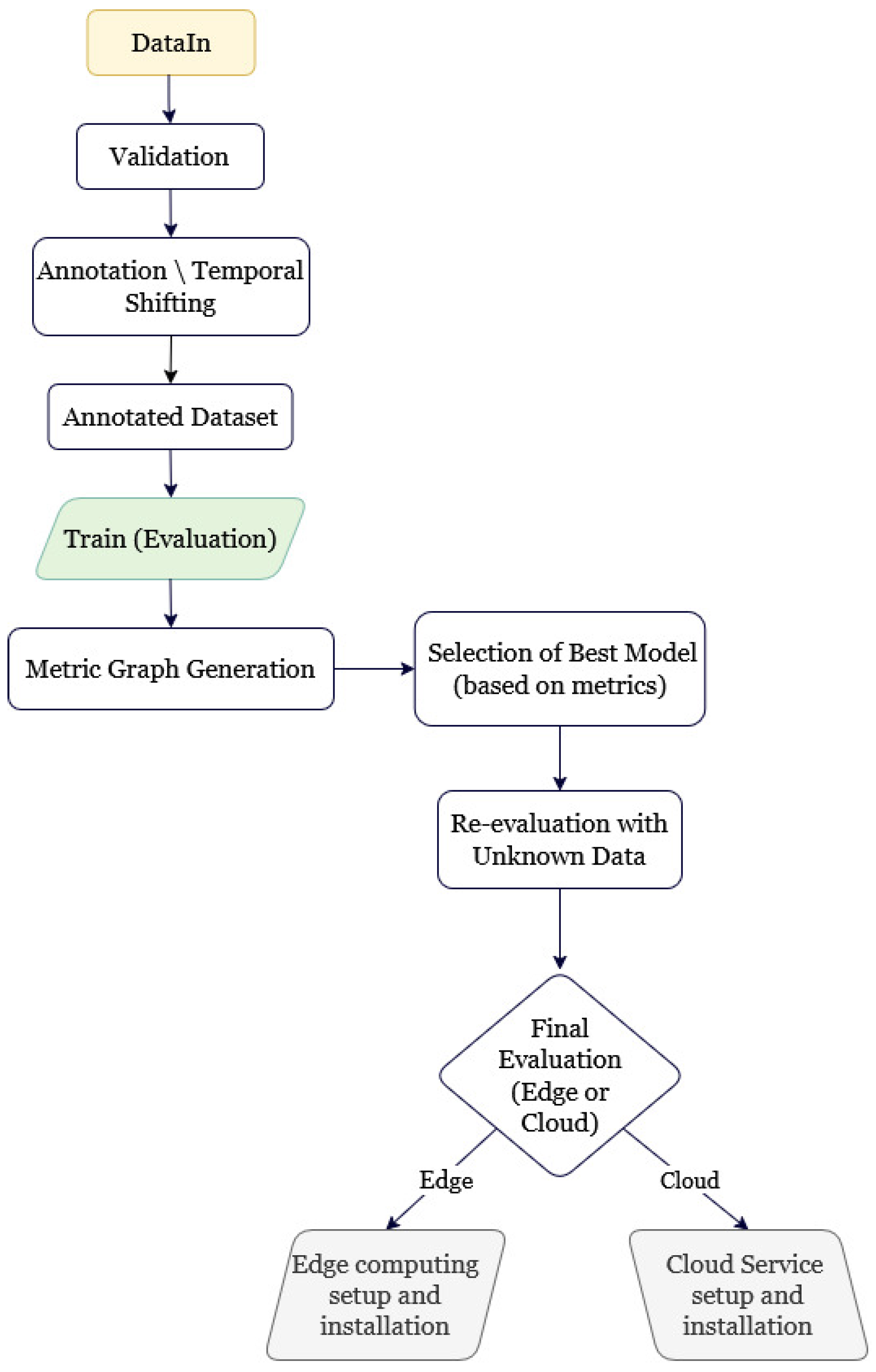
Figure 1 depicts the entire data processing and model deployment workflow that was implemented in this study. The process began with raw input data, which underwent validation and temporal preprocessing before being used to train the proposed neural network models. Depending on the forecasting scale, computational requirements, and user-specific restrictions, the most appropriate model architecture was chosen, followed by a deployment strategy targeting either edge computing environments or cloud-based platforms. This workflow ensures flexibility, scalability, and optimal utilization of the available resources. Each step of the process, from data preparation and model training to performance evaluation and final deployment, is discussed in detail in Section 2.2.1 and Section 2.2.2.

2.2.1. SlideNN Model

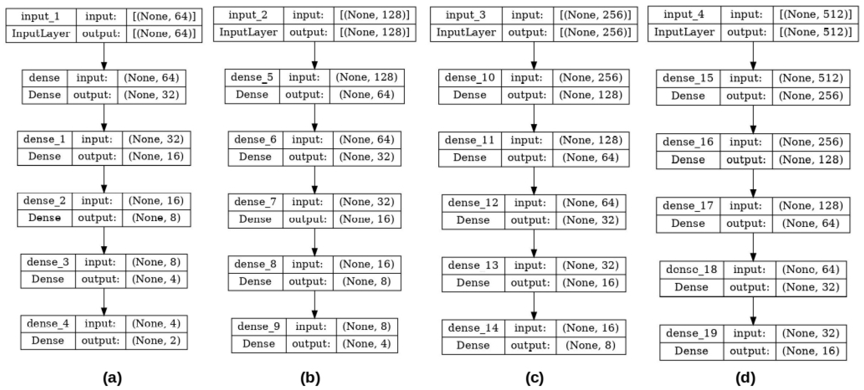
The neural network architecture, called the slideNN model, follows a specific recursive relationship that governs the structure of all four sub-model strands, defining the input size, the number of neurons per layer, and the output size similar to [45]. However, the recursive pattern in slideNN indicated a systematic leftward shift in these parameters as we progressed through the models. Specifically, each model $(M_n)$ had an input layer of size $2^i$, where $i=6, 7, 8,$ and 9 depending on the sub-model and, at each subsequent hidden layer, the number of neurons decreased following a power-of-two pattern. This reduction continued until the output layer contained $2^j$ neurons, where j ranged from 1 to 4.

The recursive relationship ruling used in the neural network models was defined as follows: Let $L_0^n$ denote the input layer size, where $n=2^k$ for some integer k. The number of neurons at each hidden layer $L_i$ follows the recurrence relation, which is given by Equation (1).

$$L_i={\displaystyle \frac{L_{i-1}}{2}},\mathrm{for}i=1,2,\dots ,d,$$

(1)

where d is the network depth such that $L_d=2^{k-d}$, representing the output layer size.

For a given model $M_j$, the relationship is expressed as

$$L_0=2^{6+j-1},$$

$$L_i=2^{6+j-1-i},\mathrm{for}i=1,2,\dots ,d,$$

$$L_d=2^{j+1},$$

where $j\in \{1,2,3,4\}$ denotes the model index, corresponding to input sizes $2^6,2^7,2^8,$ and $2^9$, respectively. This formulation captures the systematic leftward shift of the input size, hidden layers, and output size as one transitions from one model to the next. The layer architecture and configuration of each submodel are also shown in Figure 2.

2.2.2. Variable Length-GRU Model

In contrast to the stranded partitioned architecture of the NN edge device model, the GRU-based model leverages the temporal modeling capabilities of recurrent neural networks more effectively. This model is structured to handle sequential data with a fixed number of timesteps and feature attributes, and it is specifically tailored for AQI forecasting using both meteorological and particulate matter measurements. The inputs are formatted as one-dimensional vectors of length t, where t denotes the number of timesteps.

Before entering the GRU layers, each input vector is reshaped into a three-dimensional tensor of shape$(n,{\displaystyle \frac{t}{k}},k)$, where n is the number of samples, k is the number of feature attributes, and ${\displaystyle \frac{t}{k}}$ represents the sequence length. The model’s core consists of n stacked GRU layers containing m units. All but the final GRU layer returns full sequences to preserve temporal context across layers. The final GRU layer outputs a fixed-length vector representation of the input sequence, which is passed through a series of fully connected layers.

Depending on the value of m, the dense block behaves accordingly:

• For smaller values of $m\le 64$, a single dense layer with m neurons is applied.
• For larger values of $m>64$, the dense block consists of a sequence of layers starting from m. This halves in size each time until reaching 64, allowing for a gradual dimensionality reduction.

The final output layer consists of ℓ neurons corresponding to the number of AQI values predicted. The number of output neurons ℓ is not chosen arbitrarily but is derived as a function of the input sequence length t. Specifically, it follows the relation shown in Equation (2):

$$\mathsf{\ell }=2^{{log}_2(t)-5}={\displaystyle \frac{t}{32}}.$$

(2)

Formally, let $x\in {\mathbb{R}}^{t\times k}$ represent a single flattened input sequence. The transformation applied by the model is summarized in Equation (3).

$$x\stackrel{\mathrm{Reshape}({\displaystyle \frac{t}{k}})\times k}{\to }{x}^{\prime }\stackrel{\mathrm{GRU}(m)\times n}{\to }h\stackrel{\mathrm{Dense}\mathrm{block}}{\to }z\stackrel{\mathrm{Dense}(\mathsf{\ell })}{\to }\widehat{y},$$

(3)

where $x^{\prime }$ is the reshaped input, h is the output of the final GRU layer, z is the output of the dense block, and $\widehat{y}$ is the final output vector of the predicted AQI values. The architecture allows for flexible hyperparameter tuning in terms of the number of GRU layers (n), the size of each layer (m), the timestep length (t), and the number of output values (ℓ).

Different architectural results and GRU layer configurations were implemented depending on whether the model was intended for edge or cloud computing environments. These architectural designs are illustrated in Figure 3 and Figure 4, corresponding to the edge and cloud settings, respectively.

In the edge-case GRU, each configuration consistently featured two GRU layers (dual-layered with the first layer with return sequences set to True), with the number of GRU cells varying between 16, 32, 64, and 128, depending on the input size. Additional layers can be added on demand with return sequences during stranded GRU model calls, provided the number of cells remains the same (we used a single layer). All GRU layers end in a final GRU layer with return sequences equal to False and the same number of cells as the previously set GRU layers. For configurations where the number of GRU cells reached above 64 (which only occurred in the last configuration of the edge case), the subsequent dense layers were reduced by a power of two at each step until reaching 64 cells, promoting efficient computation and compactness suitable for constrained environments. The specific architecture for each configuration is illustrated in Figure 3.

A combination of the slideNN and multi-layered GRU model, with multiple strands, forms a hybrid cloud-based GRU model that adopts a deeper architecture, comprising four internal GRU models (strands). It is characterized by significantly larger GRU cell sizes per layer while pertaining a fixed ending NN in terms of the number of layers and neurons per strand, that is, the hybrid model includes GRU models, which, in our examined case, consisted of GRU models (or strands) of four layers of 1280 cells each that decreased progressively using neural network layers of neurons that had been decreased by powers of two (similarly to slideNN) of the following neuron sizes/layer: $1280\to 640\to 320\to 160\to 80$. This continued until eventually stopping once the size dropped below 64. This structure reflected the cloud setting’s capacity to support more complex and memory-intensive models, offering a broader and more expressive architecture for improved learning capacity. The structure of the examined cloud GRU counterpart is shown in Figure 4.

Finally,

Table 2. Overview of the hyperparameters for all models.

SlideNN (Edge Computing)
Submodel	Input Length	Output Length	Learning Rate	Epochs	Batch Size
1	64	2	${10}^{-4}$	400	16
2	128	4
3	256	8
4	512	16
GRU Model (Edge Computing) *
GRU Cells	Input Length	Output Length	Learning Rate	Epochs	Batch Size
16	64	2	${10}^{-4}$	50	32
32	128	4
64	256	8
128	512	16
GRU Model (Cloud Computing) **
GRU Cells	Input Length	Output Length	Learning Rate	Epochs	Batch Size
1280	64	2	${10}^{-4}$	25	32
	128	4
	256	8		35
	512	16

* All GRU configurations in the edge-case scenario used exactly two GRU layers. ** All GRU configurations in the cloud-case scenario used exactly four GRU layers.

includes the hyperparameters of each model examined in this study.

2.3. Data Collection and Preprocessing

Before delving into the specific datasets, it is important to note that the data used in this study were collected from the automatic environmental station of the Epirus prefecture (district), located at the center of Ioannina city [55]. The data spanned over 3 years, starting on 15 February 2019 and ending on 20 October 2022.

The primary air quality measurements originated from IoT-based particulate matter (PM) sensors installed in central urban locations of the city, specifically near Vilaras Street, adjacent to the Zosimaia School. The data were obtained from a 32-channel optical particle counter (APDA-372, Horiba Ltd., Kyoto, Japan) [56]. The instrument is reference-equivalent for PM_2.5 and PM₁₀ measurement according to the EN 14907 and EN 12341 standards, respectively. The sampling was conducted through a TSP sampling head equipped with a vertical sampling line, which included a particle drying system, providing mass concentrations of PM₁, PM_2.5, PM₄, and PM₁₀ fractions at hourly intervals. PM sensors of this station provide continuous hourly data for four types of particulate matter: PM₁, PM_2.5, PM₄, and PM₁₀. The instrument size measurement range was 0.18–18 µm and the mass measurement range was 0–10,000 µg/m³, whereas the measurement range was 0–20,000 ppm/cm³.

Complementary hourly average values of the meteorological data, including temperature (T), relative humidity (H), wind speed (WS), and wind direction (WD), were obtained using a collocated automated weather station. Specifically, the data were recorded by a WS300-UMB Smart Weather Sensor [57], ensuring respective measurements within the ranges −50–60 °C and 0–100% RH, as well as respective accuracy values equal to $\pm 0.2$ °C and $\pm 2\%$ RH. The wind speed and wind direction values were measured by Theodor Friedrichs & Co., Schenefeld, Germany sensors with measuring ranges equal to 0–60 m/s and 360°, respectively. The respective accuracies were equal to $\pm 0.3$ m/s at speeds larger than 15 m/s, or 2% and $\pm 2.5°$ otherwise.

Each hourly entry in the dataset formed an 8-dimensional feature vector constituting of (PM₁, PM_2.5, PM₄, PM₁₀, T, H, WS, and WD), where the PMs are the particle matter concentrations (1–10), and T, H, WS, and WD are the meteorological station measurements of the temperature, relative humidity, wind speed, and direction, respectively. These hourly vector values were then linearly interpolated to minute values, and the corresponding AQI values were calculated using the PM-interpolated minute values. These values were then used for model training and evaluation data.

Over a monitoring period of 3 years, 8 months, and 5 days, or 1344 days, taking into account leap years, the dataset comprised $1344\times 24$ = 32,256 complete hourly measurements, providing a high temporal resolution that is essential for short- and medium-term air quality forecasting. The dataset underwent a series of preprocessing steps to ensure consistency and model preparation. These included handling missing values and applying feature-wise normalization and standardization techniques to account for the unit and value range disparities across the input variables, as well as data partitioning at the minute level using linear interpolation ($\mathrm{32,256}\times 60$ = 1,935,360 total measurements).

2.3.1. Data Preprocessing

The air pollutant indicators used in this study were particulate matter (PM) concentrations, and they were divided into four distinct types based on their size: PM₁, PM_2.5, PM₄, and PM₁₀. These pollutants are significant contributors to air quality degradation, originating from various natural and anthropogenic sources, such as industrial emissions, vehicle exhausts, and biomass burning [58,59]. The dataset consists of time-series measurements of these particulate concentrations, recorded in micrograms per cubic meter (µg/m³).

Particulate matter features were subjected solely to standardization using z-score normalization. This method transforms each input variable such that it has a mean of zero and a standard deviation of one, effectively centering and scaling the data:

$$X_{std}={\displaystyle \frac{X-\mu }{\sigma }}.$$

(4)

Here, $\mu$ is the mean and $\sigma$ is the standard deviation of each PM variable computed using the training data. This transformation is significant for neural networks as it ensures that features with larger numeric ranges do not dominate the training process. It also improves the conditioning of the optimization problem and speeds up the convergence during training [60,61].

Meteorological variables are crucial for AQI forecasting as they influence pollutant dispersion, deposition, and transformation. This study incorporated temperature (°C), relative humidity (%), wind speed (m/s), and wind direction (°) [62].

For the meteorological variables, a two-stage preprocessing pipeline was implemented. The raw values of the meteorological variables were first standardized using the same z-score formula as Equation (4). Standardization was followed by min-max normalization to scale the standardized values into a bounded range between 0 and 1, as shown in Equation (5):

$$X_{norm}={\displaystyle \frac{X_{std}-X_{min}}{X_{max}-X_{min}}}.$$

(5)

This combined approach was chosen to accommodate both the need for zero-centered inputs and the benefits of scaled features within a uniform range [63]. Notably, min-max normalization was applied after standardization using the minimum and maximum values of the standardized training data to ensure consistency and to prevent information leakage.

The output dataset, consisting of future Air Quality Index (AQI) values, underwent a preprocessing strategy designed to accommodate the structure of the prediction models and improve training stability. Specifically, the number of future AQI values used as prediction targets varied depending on the model configuration. Four distinct input sizes, corresponding to 64, 128, 256, and 512 hourly data points, were selected. For each of these, the output consisted of the subsequent 2, 4, 8, and 16 hourly AQI values, respectively.

To construct the output dataset, specific rows were selected from the complete AQI time series. More specifically, for each input size, the following $2^k$ hourly AQI data, where $k=1, 2, 3,$ and 4, were chosen as prediction targets for every $2^i$ consecutive row, where $i=3, 4, 5,$ and 6. This slicing strategy ensured temporal separation between training samples and helped prevent excessive overlap in prediction windows, thereby reducing potential data leakage and autocorrelation bias during training and evaluation [64]. For further clarity regarding the input and output configurations,

Table 3. The input–output configurations used across both model architectures. Each configuration represents a specific combination of the input window size and prediction horizon applied to both slideNN and GRU models.

Configuration	Input Window (Hours)	Sampling Step (Hours)	Number of Outputs
Config 1	64	8	2
Config 2	128	16	4
Config 3	256	32	8
Config 4	512	64	16

Note: These configurations were implemented as separate sub-models in the slideNN architecture and as adjustable hyperparameter scenarios within a single GRU model.

presents a summary of the respective settings used in the prediction process.

After the slicing process, the final output dataset that was used was created, and all the AQI target values were standardized using z-score normalization in accordance with Equation (6):

$$Y_{std}={\displaystyle \frac{Y-{\mu }_Y}{{\sigma }_Y}},$$

(6)

where ${\mu }_Y$ and ${\sigma }_Y$ are the mean and standard deviation of the AQI values across the training targets, respectively.

Standardizing the output proved to be a crucial step in reducing prediction errors and stabilizing the training process [65]. Without standardization, the models exhibited significantly higher loss fluctuations and slower convergence, particularly when predicting multiple future time steps with higher variability in AQI levels.

Given that both the input features and the output values span entirely different average value ranges and measurement units, insufficient preprocessing will naturally lead—just as observed—to particularly high prediction errors and poor model generalization. Initially, only the input features were normalized and/or standardized, but the prediction loss remained notably high. Once output AQI values were also standardized, model performance improved significantly, enabling more effective learning and better predictive accuracy.

For a deeper understanding of the diversity in scales and measurement units among the variables,

Table 4. Typical value ranges for the input and output variables used in this study.

Variable	Typical Range	Remarks
PM1 (µg/m3)	0–25	Low concentration; urban sources.
PM2.5 (µg/m3)	0–35	WHO daily limit: 25; frequently exceeded.
PM4 (µg/m3)	0–50	Mid-size particles; often industrial origin.
PM10 (µg/m3)	0–100	WHO daily limit: 45; exceeds near roads.
Humidity (%)	30–90	Low under 30%; variable near water bodies.
Temperature (°C)	–5–40	Season-dependent; typically 10–30°C.
Wind speed (m/s)	0.5–10	Calm < 1 m/s; strong winds > 6 m/s.
Wind direction (°)	0–360	Circular; 0°/360° = North.
AQI	0–500	<50: good, >150: unhealthy.

was constructed, which presents the typical value ranges for each variable that was used in this study [7,15,16,66]. These ranges are based on international standards and scientific literature, supporting the rationale for proper data preprocessing prior to model training.

To maintain the integrity of the temporal structure within our dataset and to prevent any potential data leakage, we approached the division of training and validation data with careful consideration. Although the Keras framework offers a convenient validation_split parameter, its improper use can lead to leakage if the data are shuffled prior to splitting. To address this risk, we specifically set shuffle = False when training the model. This ensures that the validation set consistently comprises the most recent 20% of the data, while the training set is formed from earlier entries. This approach effectively preserves the chronological sequence of the time series, allowing the model to utilize only past data when predicting future values. As a result, we upheld the integrity of the forecasting task and prevented any occurrences of temporal leakage.

After completing the data preprocessing phase, a final reshaping step was applied to convert the input data into a format compatible with each of the two different architectures. Initially, the input was structured as a sequence of rows, where each row corresponded to a single hourly observation and included the eight known variables.

2.3.2. Preprocessing for SlideNN

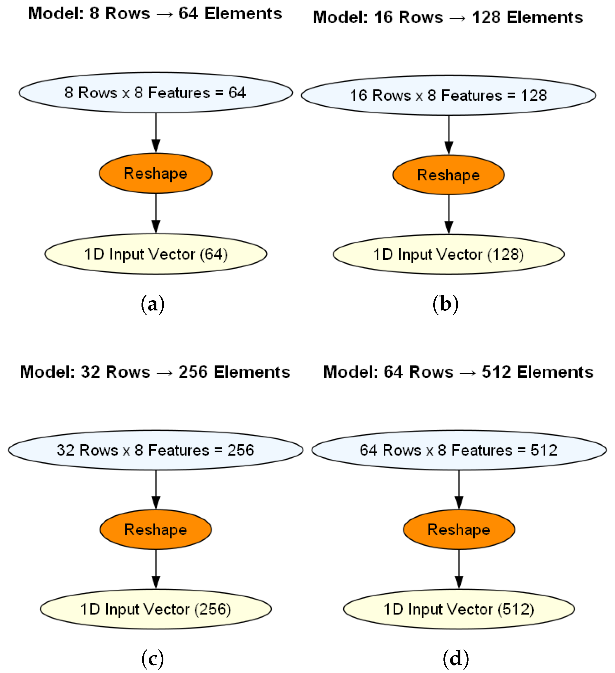
In order to construct fixed-size input vectors, consecutive groups of rows were accumulated and flattened into one-dimensional (1D) arrays. Each model configuration defined a specific number of rows to be grouped based on the corresponding input size:

• The first model combined 8 consecutive rows ($8\times 8$) into a 64-element vector.
• The second model used 16 consecutive rows ($16\times 16$), resulting in 128-element vectors.
• The third model added 32 consecutive rows ($32\times 32$), turning them into 251-element vectors.
• The fourth model used 64 consecutive rows ($64\times 64$), making 512-element vectors.

Mathematically, let $X\in {\mathbb{R}}^{n\times 8}$ be a matrix representing n consecutive hourly observations, each with 8 features. The reshaping process transforms this into a one-dimensional input vector $x\in {\mathbb{R}}^{8n}$, as shown by Equation (7):

$$x=\mathrm{reshape}(X)=[x_{1,1},x_{1,2},\dots ,x_{1,8},x_{2,1},\dots ,x_{n,8}],$$

(7)

where $x_{i,j}$ is the $j^{\mathrm{th}}$ feature of the $i^{\mathrm{th}}$ hourly record. This operation preserves the temporal order of observations while converting them into a flat format suitable for fully connected feedforward neural networks. In Figure 5, each model’s reshaping process is depicted for a better understanding.

2.3.3. GRU Model Preprocessing

Although RNNs typically require 3D input shapes to capture temporal dynamics, in this implementation, the GRU model receives the same flattened 1D input vectors as the feedforward slideNN model. Specifically, each input vector has a total temporal length (timestep) t, which results from flattening l timesteps with $k=8$ features each (corresponding to environmental conditions and particle matter concentrations), as expressed by Equation (8):

$$t=l\times k\Rightarrow l={\displaystyle \frac{t}{k}},$$

(8)

where t is the total input size; $k=8$ is the number of features per timestep, which is flattened and set with a specific order over timesteps as a 1D vector; and l is the number of effective timesteps (e.g., 8, 16, 32, or 64). Before feeding the data into the GRU layers, an internal reshaping step is applied to convert each 1D vector of shape h into a 2D matrix of shape $(l,k)$, as follows:

$$\mathrm{reshape}(\mathbf{x})=\left[\begin{array}{cccc}{x}_{1,1}& x_{1,2}& \dots & x_{1,k}\\ x_{2,1}& x_{2,2}& \dots & x_{2,k}\\ ⋮& ⋮& \ddots & ⋮\\ x_{l,1}& x_{l,2}& \dots & x_{l,k}\end{array}\right]\in {\mathbb{R}}^{l\times k}.$$

(9)

This reshaping process aligns the input format with the GRU’s expected 3D tensor shape (including batch size): $\mathbf{X}\in {\mathbb{R}}^{m\times l\times k}$, where m is the number of input samples. Importantly, while the slideNN model uses the 1D input directly, the GRU model performs this additional transformation internally to reconstruct the temporal sequence from the same flattened vector. This design ensures structural compatibility while maintaining architectural consistency across both models.

2.4. Training Process and Measures

The neural network models, as well as the GRU models, were trained using the Root Mean Squared Error (RMSE) as the loss function, which is well suited for regression tasks and has been used as the standard statistical measure to evaluate a model’s performance when it comes to meteorological and air quality studies [67,68]. RMSE emphasizes larger errors more heavily than smaller ones due to the squaring of differences. It also preserves the same units as the target variable, making it particularly effective for evaluating long-term forecasting accuracy. RMSE calculates the square root of square averages of the differences between predicted and actual values and is defined based on Equation (10):

$$\mathrm{RMSE}=\sqrt{{\displaystyle \frac{1}{n}}\sum _{i=1}^n{\left(y_i-{\widehat{y}}_i\right)}^2},$$

(10)

where n is the total number of observations, $y_i$ represents the actual value of the i-th observation, ${\widehat{y}}_i$ the predicted value for the i-th observation, and ${\left(y_i-{\widehat{y}}_i\right)}^2$ is the squared error for the i-th prediction.

The performance of the models was evaluated using three key error measures: the Root Mean Squared Error (RMSE), Mean Squared Error (MSE), and Mean Absolute Error (MAE). The RMSE was defined above by Equation (10). The Mean Squared Error (MSE) computes the average of the squared differences between the predicted and actual values. It is mathematically expressed by Equation (11):

$$\mathrm{MSE}={\displaystyle \frac{1}{n}}\sum _{i=1}^n{(y_i-{\widehat{y}}_i)}^2.$$

(11)

MSE provides a smooth and sensitive measure of the prediction error. However, larger deviations have a disproportionately higher impact due to the squaring operation. RMSE is the square root of MSE, providing a measure that retains the same units and smooth increases in error magnitude as the target variable (in this case, AQI), thereby making the error magnitude easier to interpret in real-world terms. On the other hand, the MAE is less robust to outliers, providing fair forecasting when outlier values are primarily due to measurement noise. The MAE is expressed by Equation (12):

$$\mathrm{MAE}={\displaystyle \frac{1}{n}}\sum _{i=1}^n\left|y_i-{\widehat{y}}_i\right|,$$

(12)

where $y_i$ is the actual value, ${\widehat{y}}_i$ is the predicted value, and n is the total number of predictions. This measure is particularly useful when it is necessary to interpret prediction accuracy in terms of actual AQI units. This is because MAE, as a measure, treats all errors linearly. At the same time, as meteorological and particulate matter data typically spike due to the nature of the phenomena, specifically due to the irregularity and asymmetry of climate change events, they were excluded as scenario evaluation measures.

The independent samples’ t-test evaluation was used to compare whether the means of the two model groups were statistically different. For model comparisons, Equation (13) was used in this evaluation.

$$t={\displaystyle \frac{{\overline{X}}_1-{\overline{X}}_2}{\sqrt{\frac{{\sigma }_1^2}{n_1}+\frac{{\sigma }_2^2}{n_2}}}},$$

(13)

where $\overline{X}$ is the sample mean, $\sigma$ the standard deviation, and n the sample size. Having as the Null hypothesis ($H_0$) the lack of difference between arbitrary model performances concerning the first model ($64\to 2)$, a p-value of < 0.05 rejects $H_0$ with 95% confidence.

On the other hand, Cohen’s d was used to measure the standardized difference between the two group means, expressed in units of pooled standard deviation, as captured by Equation (14).

$$d={\displaystyle \frac{{\overline{X}}_1-{\overline{X}}_2}{spooled}},spooled=\sqrt{{\displaystyle \frac{(n_1-1){\sigma }_1^2+(n_2-1){\sigma }_2^2}{n_1+n_2-2}}},$$

(14)

where ${\overline{X}}_1$ and ${\overline{X}}_2$ are the sample means of different models (Model A and B—pairwise comparison), and $spooled$ is the pooled standard deviation calculated in Equation (14) using $n_1$ and $n_2$ number of samples and the ${\sigma }_1$ and ${\sigma }_2$ of the corresponding standard deviations of Models A and B, respectively. Large effects are indicated with d values greater than 0.8, noticeable improvements are above 0.5, and negligible differences are below 0.2.

The Adam optimizer was used to train both architectures, with an initial learning rate of 0.0001 for all existing models. Adam adaptively adjusts learning rates for each parameter based on estimates of the first and second moments of the gradients, which accelerates convergence and improves stability, particularly for noisy data, such as air quality measurements. A learning rate of 0.0001 was consistently used in all AQI forecasting models due to its stability during training, especially in deep architectures and time series data. More aggressive rates, such as 0.001 or 0.01, often caused unstable training with oscillating losses, given the small dataset and complex patterns. In contrast, 0.0001 allowed for a gradual learning process, helping the networks, especially the GRU-based models and deeper slideNN variants, to converge on meaningful representations without overshooting the local minima. The slideNN model was trained for 400 epochs and used a batch size of 16, while the GRU model was trained for approximately 25–50 epochs using a batch size of 32. These values, along with the other relevant hyperparameters used in the experiments, are summarized in Table 2 for clarity.

The available data were first divided into a training set and a separate testing set. During training, 20% of the training data were set aside for validation using the validation_split = 0.2 parameter in TensorFlow. This approach ensured that the validation set was drawn exclusively from the training data while the testing set remained isolated for final model evaluation.

The appropriate neural network architecture was chosen based on the hyperparameters and the specific requirements selected by the end user, such as the desired forecast horizon (short-term vs. long-term) or computational resource limitations. At the same time, the deployment strategy was decided based on whether to use cloud infrastructure or edge computing. When the most suitable option was identified, the corresponding technical setup and installation were performed, involving either deployment on a local edge device or within a cloud environment.

3. Experimental Scenarios

The authors conducted controlled experiments using NN and recurrent NN models to evaluate and compare their proposed framework. Each model was trained separately with adjusted hyperparameters and architectural choices to investigate the performance improvements gained under different data and model configurations. Two distinct deep-learning architectures were implemented and analyzed:

• A feedforward neural network, referred to as slideNN.
• A Gated Recurrent Unit (GRU)-based architecture.

Both models were evaluated under four input–output configurations using time windows of 64, 128, 256, and 512 h as input, with corresponding prediction horizons of 2, 4, 8, and 16 h of AQI values, respectively. This enabled a consistent comparison of AQI forecasting, revealing how varying the amount of historical input data and forecast length affected model performance. The experiments were performed under identical preprocessing conditions, and both architectures were trained using standardized AQI data to ensure consistency and fairness in comparison.

The experiments were also differentiated into the two main framework computational deployment cases: Edge computing, and cloud computing. Each scenario was designed to reflect realistic use cases, taking into account constraints on computational resources and inference requirements.

Edge 

Computing case: This scenario simulates environments with limited hardware capabilities, such as embedded systems or mobile devices. Both architectures–slideNN (a feedforward neural network) and a GRU-based model architecture were tested under four distinct input–output configurations of $64\to 2,128\to 4,256\to 8,$ and $512\to 16$ (hours). The variable length GRU model was adjusted using a small number of cells (e.g., 8, 16, 32, and 64) to match the parameter count of the corresponding slideNN sub-model. Enabling a fair and direct comparison of their performance on the same resource-constrained platform.

Cloud 

Computing case: This scenario represents high-resource environments where model complexity and real-time inferences are not a limiting factor. Only the GRU-based model was tested in this case, using a larger number of cells (specifically 1280) to exploit its full representational capacity. For each of the four input–output configurations mentioned above, the GRU layer was followed by a dense NN sub-network, forming a hybrid architecture that combines deep-temporal recurrent modeling with deep-layered neural network processing.

The results of the edge GRU models were compared with those of the slideNN models for the same input–output configurations. Performance was measured using RMSE, allowing direct comparison between recurrent and feedforward approaches at matched model capacities. To initiate the evaluation process, we conducted experiments on the feedforward neural network architecture, referred to as slideNN. The model was trained and tested independently for the four input–output configurations, namely 64-2, 128-4, 256-8, and 512-16 (Figure 2), corresponding to the number of hours used for input and prediction, respectively.

3.1. Scenario I: Edge Case Evaluation (SlideNN vs. GRU)

In this scenario, we focused on environments with limited computational resources, where smaller models are preferable (edge and real-time AI). For this reason, the GRU model was tested with a small number of recurrent units (cells) selected from the set $8, 16, 32, 64 \mathrm{and} 128$. The experiment showed that the performance difference between using 8 and 16 GRU cells was negligible. As such, they are not treated as distinct cases but are instead grouped into a single category representing the smallest cell configuration.

To ensure a fair comparison, the number of trainable parameters in the edge GRU model was matched to that of the corresponding slideNN model for each input–output configuration. Specifically, four submodels of both GRU and slideNN were created and trained for input sizes 64, 128, 256, and 512, and their performance was evaluated using the Root Mean Squared Error (RMSE).

Table 5. Model configurations with the parameter count and corresponding memory size.

Configurations	Input/Output Size	Parameters (p)	Memory (KB)
1	64/2	2790 $\le p\le$ 3186	$10.9\le KB\le 12.45$
2	128/4	11,036 $\le p\le$ 11,556	$43.11\le KB\le 45.14$
3	256/8	43,848 $\le p\le$ 43,896	$171.28\le KB\le 171.47$
4	512/16	175,088 $\le p\le$ 177,872	$683.94\le KB\le 694.81$

provides each configuration’s inputs and outputs, number of parameters, and load memory sizes.

Each configuration was tested independently to compare how well each architecture performed, both in terms of training convergence and forecasting accuracy, in resource-constrained settings.

3.2. Scenario I: Experimental Results

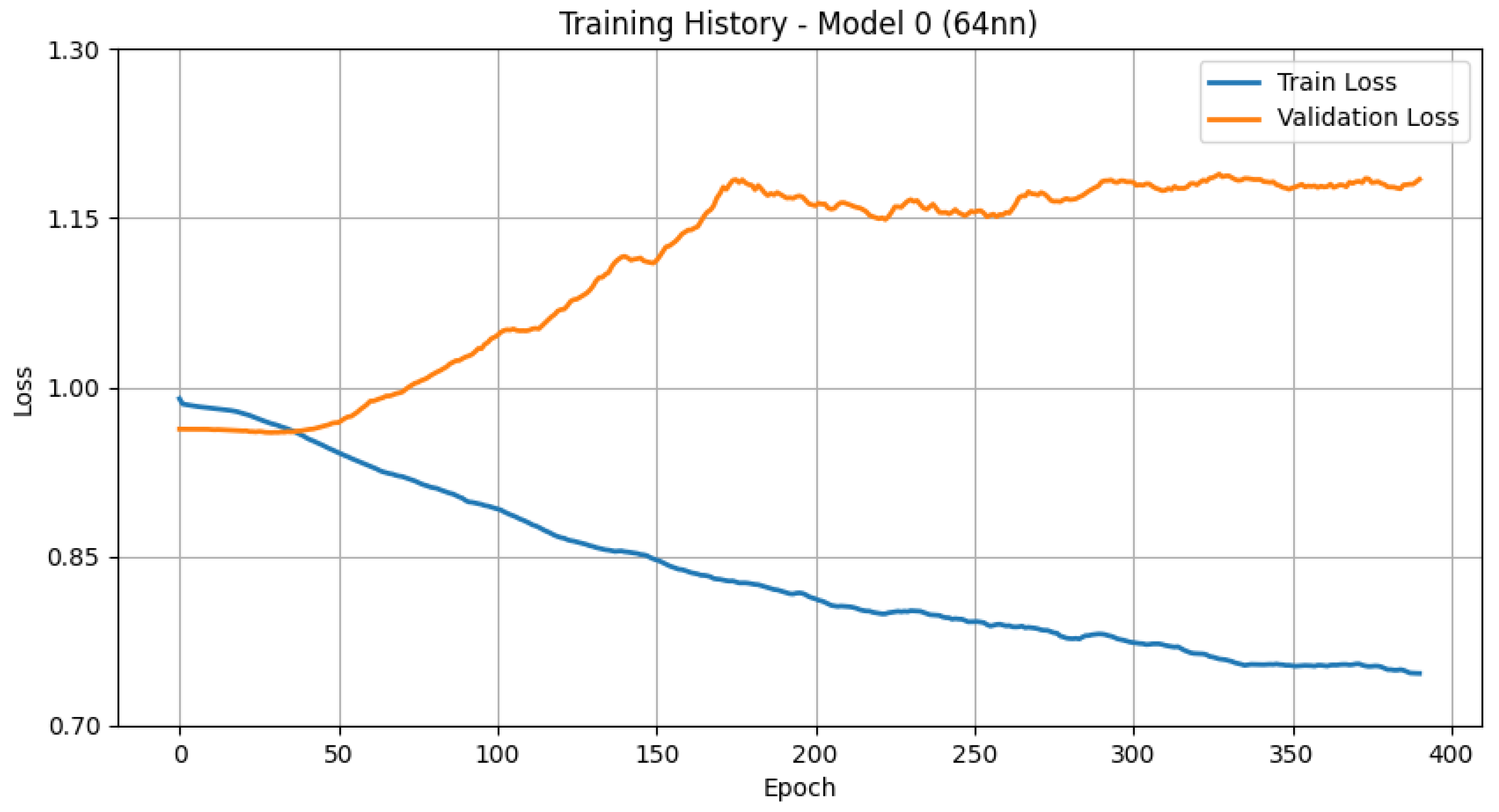
Regardless of the medium size of the training dataset, each submodel was trained for over 400 epochs to identify cases of overfitting. Since no early stopping mechanism was implemented for the slideNN model, training was deliberately extended to 400 epochs to evaluate its performance across a wide temporal range. During early experiments with fewer epochs (starting from 100), the training loss continued to decrease, suggesting room for further optimization. However, analysis of the training versus validation loss curves revealed that, after approximately 30–35 epochs, the validation loss began to increase while the training loss decreased, and it eventually surpassed it—a clear sign of overfitting. As indicative evidence, the training versus validation loss curve of a representative submodel (slideNN with input/output: $64\to 2$), as shown in Figure 6 below, clearly demonstrates this overfitting behavior. The remaining submodels (strands) exhibited similar patterns, further supporting this observation.

The resulting predictions were not highly accurate in absolute terms. However, the experiments did reveal a consistent, inductive pattern of improvement across the submodels. Specifically, as the output size increased from 2 to 16, each subsequent configuration produced better results than the previous one. The slideNN model performance improved inductively as more output steps were introduced, likely due to its capacity to capture broader temporal dependencies when given more extensive target horizons. To showcase the performance of each submodel within the slideNN architecture,

Table 6. Conservative performance measures for the slideNN model (mean ± std over 10 runs).

Submodel (Input → Output)	RMSE (Mean ± $\mathit{\sigma }$)	MSE (Mean ± $\mathit{\sigma }$)	p-Value (vs. 64→2)	Effect Size (Cohen’s d)
64 → 2	0.786 ± 0.051	0.617 ± 0.048	–	–
128 → 4	0.674 ± 0.039	0.454 ± 0.035	0.035	0.62
256 → 8	0.641 ± 0.032	0.410 ± 0.028	0.028	0.85
512 → 16	0.596 ± 0.025	0.355 ± 0.021	0.025	1.25

presents the loss (RMSE) and the respective MSE for each configuration.

The slideNN model architecture, however, showed moderate improvements (d = 0.62–1.45), with all model strands achieving statistical significance ($p<0.05$). The $512\to 16$ submodel demonstrated the strongest effect ($d=1.45, p=0.025$), though its RMSE (0.596) values were still extremely high. Furthermore, the slideNN models were faster than GRU in terms of training, inference, edge device implementation, and memory residence occupation. Therefore, slideNN was found to be the model that can infer results, even in 8bit microcontroller units (MCUs), with the least device requirements.

Following experimentation on the slideNN architecture, we conducted a corresponding series of evaluations to capture the temporal patterns using a GRU-based Recurrent Neural Network model. GRU was selected as it better at capturing, without suffering from the vanishing gradient problem, long-range dependencies than RNNs. It maintains fewer gates than LSTMs (two instead of three and as cell states), resulting in faster inferences and reduced memory usage.

Four distinct input–output configurations were employed—64-2, 128-4, 256-8 (Figure 3), and 512-16—ensuring direct comparability between the two architectures. In addition to the input and output window sizes, the GRU model introduced two more key hyperparameters: the number of GRU cells and the number of internal layers. For each configuration, the number of cells was carefully selected so that the total number of trainable parameters closely matched that of its slideNN counterpart. The selected values were 16, 32, 64, and 128 cells for the respective input–output pairs, which can run on 32-bit microprocessor devices with at least 1–2 MB of available RAM.

Regarding the internal GRU layers, in the context of the resource-constrained edge computing scenario, this hyperparameter was set to a constant value of two layers across all configurations. This design choice was also driven by the need to maintain a parameter count comparable to that of the corresponding slideNN models, ensuring a fair and consistent basis for comparison.

Training was performed over 50 epochs with a batch size of 32. In the GRU model, both in the edge and cloud (hybrid model) cases (see Scenario II, Section 3.3), using an early stopping function with patience of 3 epochs of no RMSE change being present (≤10⁻³) helped to select the most appropriate training epochs for the most desirable results.

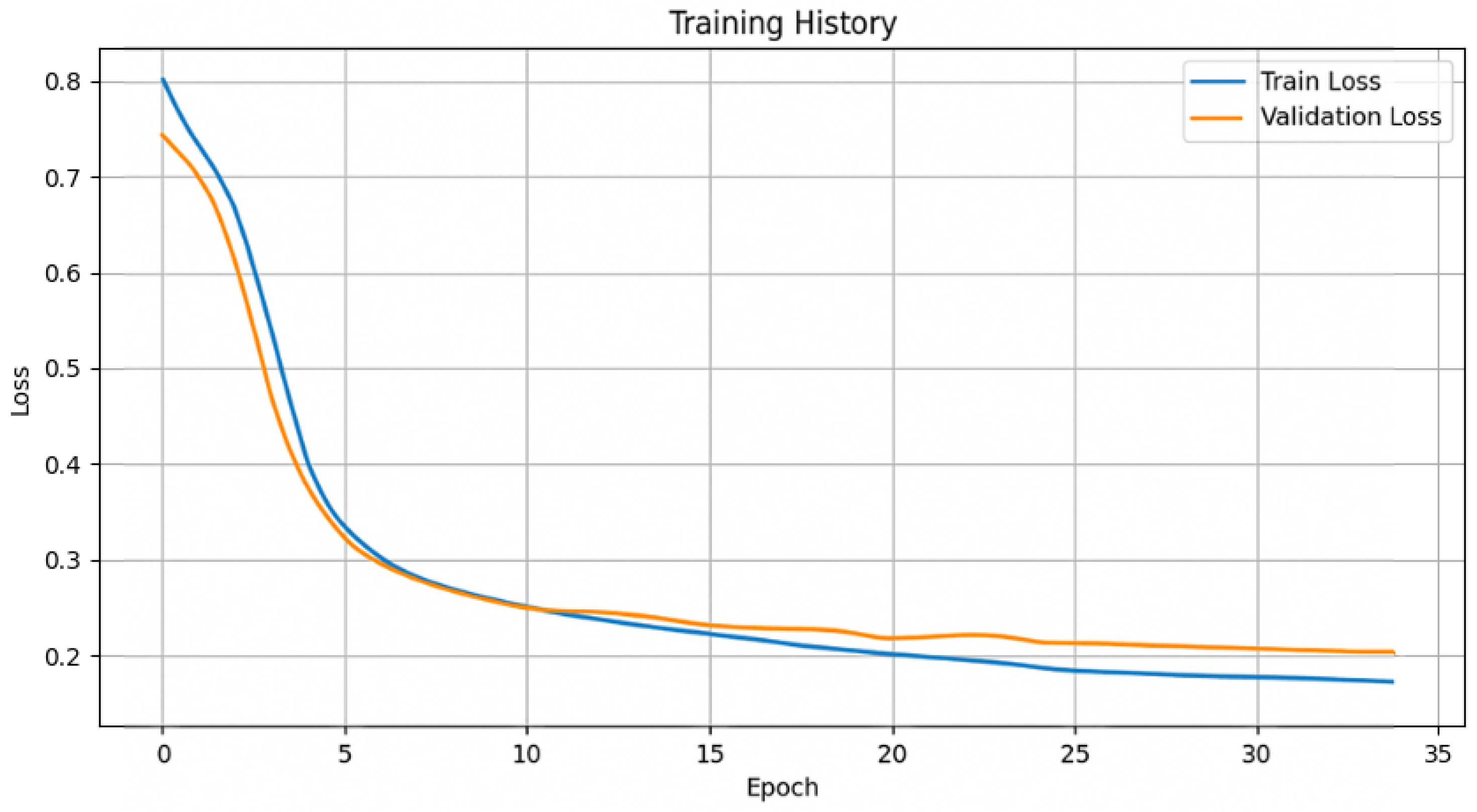
Compared to slideNN, the GRU architecture required significantly fewer epochs to converge, largely due to its recurrent structure, which is inherently more capable of capturing the temporal dependencies in sequential data. The problem of overfitting did not occur in this case, and the corresponding training versus validation loss curve graph, as shown in Figure 7 below, further confirmed this finding. In this instance, the model with an input/output configuration of $256\to 8$ was chosen because it showed a significant improvement over its slideNN counterpart strands and demonstrated practical utility, despite being one of the larger models in an edge environment.

Maintaining the same parameter settings across both sub-scenarios, it became evident that the GRU-based architecture consistently achieved better results compared to the slideNN model, regardless of the input–output configuration. A clear inductive improvement was still observed in the prediction performance as both the number of timesteps and GRU cells increased. This trend was reflected in the gradual reduction in errors. These findings indicate that the GRU architecture benefits substantially from increased complexity, improving its ability to capture long-term dependencies and patterns within the data. The performance results of each configuration of the GRU architecture for edge computing are shown in

Table 7. The conservative performance measures for the GRU model in edge computing (mean ± std over 10 runs).

Configuration (Input → Output)	RMSE (Mean ± $\mathit{\sigma }$)	MSE (Mean ± $\mathit{\sigma }$)	p-Value (vs. 64→2)	Effect Size (Cohen’s d)
64 → 2	0.599 ± 0.042	0.369 ± 0.038	–	–
128 → 4	0.507 ± 0.028	0.262 ± 0.022	0.028	0.85
256 → 8	0.317 ± 0.015	0.101 ± 0.008	0.022	1.65
512 → 16	0.233 ± 0.011	0.055 ± 0.004	0.020	1.90

.

As shown in Table 7, all the configurations remained statistically significant ($p<0.05$) with effect sizes constrained to $d<2.0$. The $128\to 4$ variant showed a moderate effect of d = 0.85, while larger models achieved $d>1.65$, confirming their practical utility despite edge hardware limitations. The $512\to 16$ model retained the strongest improvement (RMSE = 0.233, d = 1.90, p = 0.020).

A comparative plot of the RMSE values was constructed to visually assess the relative performance of the two architectures across different input–output configurations. Figure 8 illustrates how the prediction error, as measured by RMSE, evolved for each configuration (1 through 4, meaning the four different input and output windows discussed previously) for both the feedforward slideNN and the recurrent GRU model. Each point on the curves corresponds to a specific model setup, with the x-axis representing increasing input and output size and the y-axis showing the corresponding RMSE. This comparison highlighted the general trend of the performance improvement in both models as the amount of historical data increased while also showcasing the consistent superiority of the GRU architecture in minimizing prediction error across all scenarios.

As shown in Figure 8, the GRU models outperformed all slideNN models in terms of RMSE when using the same dataset, data transformations, and training parameters. For Configuration 1 of 8 of the vectorized timestep inputs of environmental measurements ($T,H,W_s,Wd,PM1,PM2.5,PM4,$ and $PM10$), the stranded GRU model presented 25% less loss than the slideNN model. A similar profile was also maintained for Configuration 2 (strand), which had 16 timestep inputs. Then, for the 32 and 64 temporal input configurations, the GRU models outperformed even the slideNN models, offering 50% and 80% less loss, respectively.

Furthermore, to achieve the good aforementioned slideNN losses (expressed by RMSE), the model was trained over 400 epochs concerning the GRU models’ 50 epochs, which was achieved using a stop training condition of three epochs patience and a delta value to qualify as an improvement of 0.001. This indicates that GRU models can distinguish temporal patterns more effectively than plain NN models and train significantly faster than NN models. Regarding dataset training epochs, the GRU model training was at least eight times faster compared to slideNN.

In conclusion, under similar-sized models with the same number of parameters and memory sizes, the GRU models performed at least 25% better than the NN models for small temporal timesteps and at least 50% better for medium temporal timesteps. Looking at the inference times, both models performed similarly in their corresponding configurations, showing no significant delays (similar inference times).

3.3. Scenario II: Cloud Case Evaluation

Following the framework experiment on the cloud cases and the better performance results achieved by the GRU models compared to slideNN, we conducted experiments centered on significantly larger parameter sets, deeper internal layers, and a more complex hybrid GRU-NN architecture. These configurations were more effectively implemented using cloud computing resources, which provide the necessary resources in terms of memory and processing power to support training, loading, and short inference intervals. In this scenario, only the GRU architecture was employed, as it has been proven to be more suited for handling long temporal sequences and complex sequential dependencies. Since GRU outperformed the NN models, maintaining a better forecasting profile of the minimal loss in variable timesteps, only the variable GRU architecture was evaluated across all four input–output window configurations (64–2, 128–4, 256–8, and 512–16) to provide a comprehensive comparison and to examine how the architecture performs under varying temporal resolutions and forecasting horizons when deployed in a cloud-based environment.

Transitioning to a cloud GRU architecture that broadens model instantiation memory requirements and allows for real-time inference resulted in a substantial increase in the number of trainable parameters compared to the edge computing scenarios. This increase was attributed to the higher number of GRU cells and the deeper, more complex network structure employed in these experiments. In cloud-based model deployment, a widely accepted threshold for qualifying a model as appropriate for cloud inference is a parameter memory size exceeding 100 MB, as mentioned in [69]. To illustrate this difference,

Table 8. Model configurations with the parameter count and corresponding memory size.

Configurations	Input/Output Size	Parameters (p)	Memory (MB)
1	64/2	37,196,882	141.89
2	128/4	37,197,044	141.9
3	256/8	37,197,368	141.9
4	512/16	37,198,016	141.9

below summarizes the number of parameters and their corresponding memory size for the two configurations used in this scenario. All of the models maintained almost similar parameter sizes while increasing the timestep depth and forecasting lengths similarly to the slideNN and edge-GRU outputs of the edge computing scenarios.

3.4. Scenario II: Experimental Results

The cloud GRU model’s performance was evaluated, with a focus on its ability to produce accurate long-range AQI forecasts, using RMSE. Unlike the edge scenario, the model size was not constrained here, enabling the architecture to fully exploit the available computational resources. Furthermore, it was configured with 1280 GRU cells and connected to a sub-network with decreasing neuron counts, forming a hybrid recurrent–dense architecture. This design aims to combine the temporal learning capability of GRUs with the dense layers’ hierarchical feature abstraction strengths. The dense sub-network used here mirrored the layer structure of the corresponding slideNN models: fully connected layers with neuron counts decreasing by a factor of two at each step (Figure 4).

This scenario treated the number of internal GRU layers as a key hyperparameter, as deeper architectures increase model complexity and are better suited for cloud-based experimentation. An initial configuration with two layers was tested but later discarded as it failed to utilize the cloud environment’s computational advantages fully. Consequently, configurations with three and four layers were selected to explore the benefits of increased model depth; ultimately, four layers proved ideal for these experimental cases. The number of training epochs also varied depending on the model setup, ranging from 25 to 40 based on the conditional training termination criterion, which is reached when a small learning rate value is achieved.

Performance outcomes were analyzed compared to the best-performing edge GRU configurations. Across all configurations evaluated in the cloud-based setting, architectural and training modifications were applied to scale the models appropriately beyond their edge-based counterparts. A key adjustment involved significantly increasing the number of GRU cells, as it became evident that timestep size alone contributed relatively little to the total parameter count compared to other hyperparameters, a thing that can be assumed even by looking at the difference in memory size between the edge configurations (Table 5). The GRU cell size was scaled up for each configuration to ensure the models reached a substantial memory footprint suitable for cloud experimentation [69]. In line with this approach, the internal architecture was also deepened by increasing the number of GRU layers, typically favoring setups with three or more layers to leverage the higher capacity and representational power available in cloud environments.

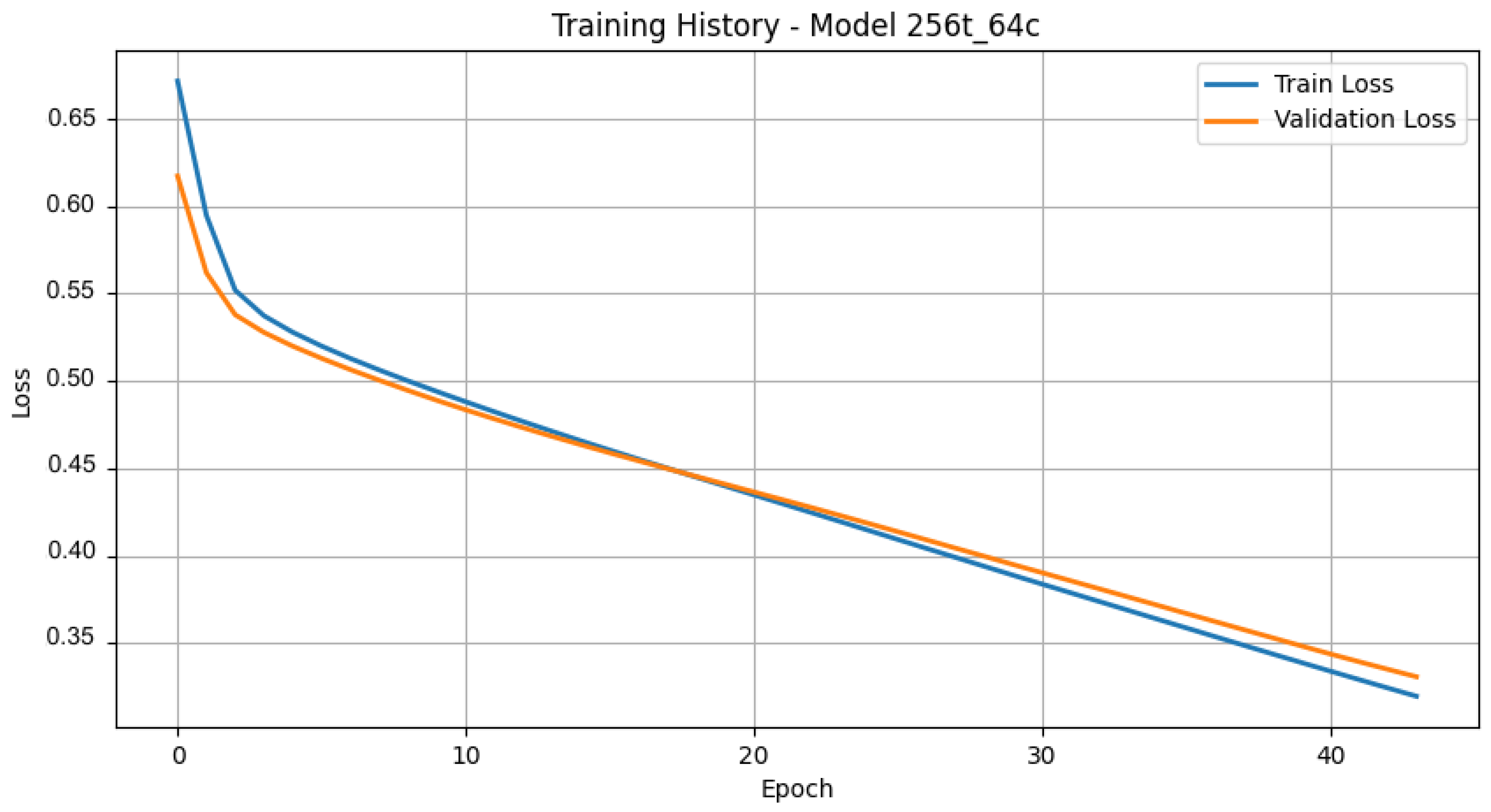
While the training duration varied slightly across configurations, most of the models were trained for approximately 25 to 40 epochs. However, the training histories indicated that the validation loss plateaued well before the final epoch. This suggests that the models had already captured the most relevant patterns earlier in training, implying that fewer iterations could achieve satisfactory performance. The same behavior was observed consistently across the configurations: in the first two setups, the validation performance plateaued around the 30th to 35th epoch, allowing the number of training epochs to be safely reduced to 25 without a loss in model quality. Similarly, in the two larger configurations, performance stabilized by the 40th epoch, which justified reducing training to approximately 35 epochs, thereby improving training efficiency and maintaining predictive accuracy (minimal RMSE loss). The training history graph of the model with input/output configuration $512\to 16$ is presented in Figure 9, showing the training and validation loss curves, which provided insight into both the ideal epoch for training this model and its fitting condition. None of the cloud hybrid GRU-NN configurations showed signs of overfitting as both the training and validation curves moved smoothly, linearly, and in proportion to each other.

As shown in

Table 9. Performance measures with statistical validation for the GRU architectures (mean ± std over 10 runs).

Configuration (Input → Output)	RMSE (Mean ± $\mathit{\sigma }$)	MSE (Mean ± $\mathit{\sigma }$)	p-Value (vs. 64→2)	Effect Size (Cohen’s d)
64 → 2	0.468 ± 0.032	0.226 ± 0.021	–	–
128 → 4	0.334 ± 0.018	0.114 ± 0.009	<0.008	1.45 (small)
256 → 8	0.213 ± 0.011	0.046 ± 0.003	<0.007	2.25 (medium)
512 → 16	0.201 ± 0.009	0.041 ± 0.002	<0.009	2.40 (medium)

, all the p-values of < 0.01 indicate that the performance improvements were statistically significant. As was also expected, the evaluation results outperformed those of their edge-based counterpart, as summarized in Table 9. While maintaining statistically significant improvements (all p < 0.01), the adjusted effect sizes still revealed substantial practical differences. The $256\to 8$ model showed a medium effect (d = 2.25), with the $512\to 16$ variant demonstrating marginally greater impact (d = 2.40). These effects exceeded Cohen’s threshold for large effects (d > 0.8) by 1.8–5 times, confirming the engineering significance of the model’s temporal depth scaling.

The cloud-based GRU models consistently outperformed their edge counterparts across all input–output configurations while using the same datasets, data preprocessing, and training setups. In the smallest setup (64 → 2), the cloud GRU achieved an RMSE of 0.468, representing a 21.9% improvement over the edge model’s 0.599. As the sequence length increased, the performance advantage of the cloud GRUs became even more apparent. For the 128 → 4 configuration, the RMSE was 34.1% lower, and, for 256 → 8, the reduction remained significant at 32.8%. Even in the largest configuration (512 → 16), where gains typically diminished, the cloud GRU model still achieved a 13.7% reduction in RMSE compared to the edge model. These results highlight the scalability and increased effectiveness of GRU models when more computational resources and memory are available. The cloud GRUs learned more robust temporal patterns due to their greater capacity.

As a result, the cloud-based GRUs outperformed the edge GRUs in terms of predictive accuracy across all tested configurations, offering up to 34% lower RMSE in mid-range settings and still delivering gains even in high-timestep conditions, with comparable inference times across both environments.

4. Discussion

From the author’s experimentation regarding the GRU cloud and edge models, as expected, the cloud-based GRU models demonstrated consistent superiority over the edge implementations, with RMSE improvements scaling from 21.9% ($64\to 2$) to 34.1% ($128\to 4$) (Table 7, Table 8 and Table 9). This performance gap narrowed at larger configurations (13.7% for $512\to 16$), suggesting diminishing returns from cloud resources for long-sequence predictions. Notably, the cloud $256\to 8$ model achieved a 32.8% lower RMSE (0.213 vs. 0.317) with 2.8 times more parameters (37.2M vs. 43.9K), highlighting the cloud’s ability to leverage increased capacity for mid-range temporal patterns.

While the cloud models required more than 100 MB of memory (see Table 8), tje edge GRUs maintained a small footprint of 700 KB (see Table 5), with a proportional accuracy loss. The $512\to 16$ edge configuration (RMSE = 0.233) achieved 80% of the cloud model’s accuracy (RMSE = 0.201) using 0.5% of the parameters, demonstrating exceptional efficiency for resource-constrained deployments. This suggests edge GRUs are viable when cloud latency or costs are prohibitive, particularly for shorter prediction horizons. On the other hand, slideNN models trained on a small number of epochs are suitable for edge devices, such as ultra-small microcontroller units, providing fair forecasting accuracy results.

Despite their larger size, the cloud models converged in 25–40 training epochs compared to the edge GRUs’ 50 epochs and slideNN’s 400 epochs. This accelerated convergence (Figure 8) stems from the cloud’s ability to process larger batches (32 vs. edge’s 16) and exploit parallelization. However, the edge models showed more stable training curves, with lower variance in the final RMSE ($\pm 0.011$ vs. cloud’s $\pm 0.015$ for $512\to 16$), indicating better generalization under hardware constraints.

The choice of batch sizes, specifically the batch values of 16 and 32, was primarily driven by established well-documented performance and use in deep learning applications. For the slideNN model, a batch size of 16 was selected primarily due to its better generalization capabilities, as the model demonstrated increased difficulty in retaining useful information. Furthermore, this choice was motivated by the reduced memory consumption since the model is intended for deployment on resource-constrained edge devices and to moderate overfitting issues observed during training, as discussed in the experimental results of scenario detailed in Section 3.2. In contrast, the GRU-based model exhibited greater stability during training, did not suffer from overfitting, and had higher memory requirements. Therefore, a batch size of 32 was deemed more appropriate for this model.

A cross-scenario analysis revealed a clear trade-off: the cloud models reduced the root mean square error (RMSE) by 21–34% but required 150–200 times more memory and 3–5 times more energy per inference. For time-critical applications, such as real-time Air Quality Index (AQI) alerts, edge GRUs offer the best balance between energy consumption and accuracy. It is important to note that cloud models are the offline analysis AI tools used by latency-tolerant systems. This highlights the importance of developing architecture-specific deployment requirements and instructions tailored to specific use cases.

Table 10. Key GRU model comparisons based on accuracy, efficiency, and edge vs. cloud deployment.

Model	Configuration	RMSE	Parameters	Memory	Insights
Cloud GRU-NN	128 → 4	0.334	~37 M	~141 MB	Best RMSE gain (34.1%) over edge,
					ideal for mid-range forecasts
Edge GRU	256 → 8	0.317	~44 K	~171 KB	Best edge trade-off for moderate
					horizon with minimal resources
Edge GRU	512 → 16	0.233	~175 K	~690 KB	Most efficient: achieves 80% of
					cloud accuracy with
					just 0.5% of the parameters
Cloud GRU-NN	512 → 16	0.201	~37 M	~141 MB	Highest accuracy, but $200\times$
					larger in terms of size

summarizes the aforementioned conclusions and contains the strongest models. Each model was evaluated based on different criteria, such as efficiency, accuracy, and resource availability. The models were compared with each other, offering insights into their distinct practical utility.

The mixing of GRU and dense neural layers in the GRU-NN architecture (hybrid model) focuses on the complementary strengths of each previously modeled GRU and slideNN model component. On the one hand, the slideNN model (a plain feedforward network) demonstrated a moderate ability to generalize temporal dependencies, particularly as the output horizons increased. As seen in Table 6, the performance improved progressively with broader output ranges, suggesting that slideNN benefits from inductive learning over extended targets. However, it also suffered from slower convergence, higher susceptibility to overfitting, and limited temporal abstraction capabilities, requiring a large number of training epochs to achieve modest reductions in loss.

In contrast, the GRU-based model exhibited superior temporal modeling capacity and training efficiency. As detailed in Table 7, the GRU configurations consistently outperformed their slideNN counterparts, achieving significantly lower RMSEs (e.g., 0.233 vs. 0.596 for the $512\to 16$ configuration) and larger effect sizes (up to d = 1.90). Notably, the GRU models required only 50 epochs with early stopping to achieve these results, indicating faster and more robust convergence. For identical input–output sizes and training conditions, the GRU models offered 25–80% lower loss, demonstrating a much stronger capacity for long-term temporal pattern extraction.

Combining these architectures in a unified GRU-NN model enhances their strengths: GRUs serve as temporal feature extractors, while subsequent dense layers support non-linear mappings and noise smoothing. This hybridization improves both predictive accuracy and training stability, as verified in Scenario II (cloud case detailed in Section 3.4), where GRU-NN consistently outperformed GRU-only and NN-only baselines across all configurations. These findings validate the architectural synergy and justify the hybrid design beyond simple stacking, supporting the added value of combining recurrent and dense mechanisms in air quality forecasting tasks.

Several recent studies have explored deep learning models for predicting the Air Quality Index (AQI), providing valuable benchmarks to assess the performance of this model. For instance, the LSTM-based model presented in a conference paper by [70] achieved an 8-hour AQI prediction with a best root mean square error (RMSE) of 12.38 using PM_2.5, PM₁₀, O₃, CO, temperature, and relative humidity as input variables. Our GRU model achieved a comparable 8-hour RMSE of 0.212 (equivalent to 12.41 when destandardized). While its accuracy is similar to that of the LSTM model, our GRU model is more computationally efficient because of its lighter architecture. Additionally, our model incorporates extra meteorological variables, such as wind speed and direction, which were not included in this study. This integration could enhance the model’s generalizability and robustness across various environmental contexts.

Additionally, the hybrid LSTM-GRU model presented in the study published in Environmental Pollution [71] examined a broader spectrum of pollutants, such as O₃, CO, NO₂, SO₂, PM_2.5, and PM₁₀, in addition to various meteorological factors, like temperature, wind speed, and relative humidity. Nonetheless, despite this expansive dataset, their model produced RMSE values ranging from 57.77 to 51.36, which is significantly higher than the RMSE of 0.334 in this study (corresponding to a 19.47 destandardized RMSE). Furthermore, their MAE remained high at 36.11, highlighting the superior predictive accuracy of our model, even while working with a more focused selection of pollutants. Although the detailed prediction horizon was not explicitly outlined in their work, it appeared to encompass several hours over multiple time steps; however, a more in-depth review of their methodology would be necessary for definitive validation.

Finally, a recent short-term study [72] explored hourly Air Quality Index (AQI) predictions using a CNN-Bi-LSTM model. Their research utilized a dataset that included NO₂, CO, O₃, SO₂, PM₁₀, and PM_2.5, as well as demonstrated strong performance over limited timeframes. Their study setup was similar to our work’s $64\to 2$ h configuration, which predicts the AQI over the next two hours. Although the CNN-Bi-LSTM model performed well on its dataset (1036A), with a root mean square error (RMSE) of 38.9324, our hybrid GRU-NN model achieved comparable or even improved predictive performance, with an RMSE of 0.456 (27.07 when destandardized). Additionally, our model features a simpler architecture and requires fewer computational resources.

The proposed models’ applicability for predicting AQI values using meteorological and particle matter concentrations may differ only in the quantity and placement of meteorological stations monitoring the microclimate and particle concentrations that occur due to ground topography, meteorological patterns, population density, and pollutant type sources [73,74].

For example, Ioannina City is a basin and is not overcrowded. Therefore, a 10 km grid or microclimate monitoring station equipped with particle sensors can adequately cover such an area. On the other hand, big cities, like Athens, require a much denser monitoring grid to address all the issues mentioned previously. Therefore, the transferability of air quality prediction models between cities, their accuracy limitations, and their practical use for decision making depend strictly on the grid of stations used to deliver more accurate local predictions of uniform characteristics in bounded environments in terms of pollutants and environmental conditions. In a densely sensing monitoring network, if focusing on localized area predictions, the proposed model can be effectively transferred if local area data are used to train the model setup for either edge device or cloud use.

5. Conclusions

This paper presents a forecasting framework for predicting localized air quality indices. The framework utilized deep learning NN models and Recurrent Neural Network models to provide predictions using, as inputs, particle matter measurements from particle matter IoT devices and environmental conditions acquired by meteorological sensory measurements of temperature, humidity, wind speed, and wind direction.

The framework differentiates between cloud-based and device-level predictions. This differentiation necessitates the application of different types of models to edge devices, given their limited computational capabilities and memory sizes. To support their framework, the authors implemented two different deep learning models that accept the same types of data inputs and provide similar AQI forecasting outputs as the framework proposes. Upon data partitioning and transformations on the different types of measurements used as inputs, the two implemented models are a neural network model handling multiple strands, called slideNN, and a variable-timestep length GRU model.

Both models were investigated for edge device implementations across four distinct time steps and various forecasting output configurations. From the experimental results, the GRU models outperformed the slideNN models by at least 25–80% in less loss, following an increasing performance curve as the number of timesteps increased. Taking as input the better performance of the edge GRU models, the authors transformed their model implementation to implement a variable GRU model, where the number of cells per layer is substantially higher, followed by several NN layers that are posed automatically based on the number of GRU cells on the last layer. This cloud-based hybrid variable GRU-NN model was investigated in terms of loss over timesteps and cross-compared with the losses achieved by smaller edge computing GRU models. From the experimental results, the GRU-NN cloud model achieved its highest relative performance gain in the 128 × 4 configuration, where it reduced the RMSE by approximately 34.1% compared to the corresponding edge GRU model (0.334 vs. 0.507). In this respect, all cloud-based GRU models outperformed their corresponding edge-computing counterparts with a mean value of 25.6%.

The authors set, as a limitation, the fact that a bigger dataset may also contribute to further accuracy gains, significantly reducing RMSE losses. The authors believe this would favor cloud-computing models; nevertheless, they consider future work to be thoroughly examined. Furthermore, the authors propose a fine-grained examination of their framework as future work, utilizing particulate matter IoT devices and microclimate monitoring meteorological stations to form kilometer-level grids.