Continuous Electrical Resistivity Tomography Monitoring in Waste Landfill Sites with Different Properties and Visualization of Water Channels

Abstract

This study aims to obtain findings on the internal water behavior, the presence of water channels, and the degree of washout due to rainfall infiltration in Japanese municipal solid waste (MSW) final disposal sites. Electrical resistivity tomography (ERT) monitoring and undistributed waste sampling for X-ray computed tomography (X-ray CT) analysis were conducted in the field. The study sites were targeted at Site A, which is mainly composed of non-combustible residues, and Site B, which is mainly composed of incineration ash. The time-dependent resistivity distributions obtained from real-time ERT monitoring were effective for us to understand the water content distribution after water infiltration during water injection tests. As a result, the global flow behavior and the local water channel flow were determined. In addition, X-ray CT analysis of the undisturbed waste samples obtained from the sites clarified the different pore structures, indicating the possibility of more advanced washing out at Site A than at Site B. Furthermore, the soil cover layer and gas extraction wells had a significant effect on the resistivity structure with respect to water flow behavior. Since soil cover layer and gas extraction wells are significant factors affecting waste stabilization by washout, it is suggested that these factors should be considered in the design and maintenance of landfills.

1. Introduction

In the maintenance and management of final disposal sites for municipal solid waste (MSW), it is essential to appropriately monitor the stabilization condition of landfilled waste. The washout of pollutants due to rainwater infiltration and the occurrence of water retention within the landfill are critical factors affecting the degree of landfill stabilization [1]. Delays in landfill stabilization can have a direct impact on practical problems such as longer maintenance periods and cost increases. In Japan, almost all combustible general waste, except plastic, is incinerated as an intermediate treatment, while plastic, glass, and ceramic waste that cannot be recycled is crushed. As a result, the main landfill wastes are incineration ash and non-combustible residues.

Numerous studies have been conducted on the washout of pollutants in landfills. It is well-known that organic substances and heavy metals are present in high concentrations in the leachate in the early stages of landfilling [2], and, therefore, methods are required to understand these dynamics.

Traditionally, monitoring wells have been installed to investigate internal hydrological conditions and water quality, but the information obtained is primarily point-based and one-dimensional, and there are limitations in understanding the two-dimensional and spatial infiltration behavior. To address this issue, electrical resistivity tomography (ERT), a physical exploration technique, has gained attention as a method capable of visually representing changes in underground water content on a two-dimensional scale [3].

ERT involves installing multiple electrodes on the ground surface, repeatedly injecting current and measuring potential differences, and estimating the spatial distribution of resistivity through inverse analysis. Resistivity is a parameter that indicates how difficult it is for electric current to flow through soil. The current flow depends on the material composition and water content of the porous material, as well as other factors. In recent years, inverse analysis techniques have evolved significantly, including specialized 3D annular electrode configuration for the detection of leachate channel [4] and 4D inverse analysis considering temporal continuity [5], optimal electrode placement based on sensitivity distribution [6], and improved computational efficiency through the introduction of unstructured meshes and wavelet compression [7], enabling faster and more accurate estimation of resistivity distributions. In addition, for phenomena where temporal changes proceed in one direction, methods have been proposed that introduce positivity constraints or asymmetric time constraints to suppress noise-induced artifacts and extract physically consistent changes in subsurface structure [8].

ERT has demonstrated its effectiveness in hydrological and geological studies [9,10,11,12]. Particularly in the field of waste landfill sites, it has been applied to underground structure surveys [13], detection of not only leachate distribution in landfill sites [14,15] but also washout pathways in unmanaged landfill sites [16], evaluation of rainwater infiltration reduction by geomembranes [17], sensitivity analysis of liner failure [18], and quantification of the influence of geomembranes as boundary conditions on inverse analysis [19], the relationship with landfill gas of CH₄ emission [20], and the temperature during waste biodrying process [21]. Notably, Helene et al. demonstrated that ERT monitoring at a landfill could describe leachate infiltration and their flow pathway [22].

However, there are few cases where not only the results of ERT surveys have been compared across multiple sites with different landfilled wastes, but also the application of temporal and spatial high-resolution ERT monitoring has been used for exploring a water channel in landfill. To investigate the influence of the pore structure of landfill layers on ERT results at different sites, this study collected undisturbed samples and performed X-ray CT analysis. This study is novel in that continuous ERT and X-ray CT analysis were conducted at two sites with different types of waste. There are significant differences in the time series of the ERT surveys, as the washout rate varies depending on the type of waste landfilled. If these differences can be clarified, it will be possible to estimate the types of waste deposited in a section of a large landfill when an ERT survey is conducted on that section. We will determine whether washout is relatively fast or slow at that location.

This study focused on two landfills managed and operated by local governments with different characteristics: Site A, primarily composed of non-combustible residues, and Site B, primarily composed of incineration ash. We used ERT to visualize and monitor the rainwater infiltration behavior at each site. At both sites, the aim was to gain qualitative and quantitative insight into the internal water behavior, the presence of “water pathways,” and the progress and stabilization of washout processes by analyzing the spatiotemporal changes in resistivity obtained from water injection tests.

2. Methods

2.1. Landfill Sites Surveyed

In this study, we conducted rainwater infiltration monitoring using ERT at two landfill sites with different characteristics. The outline of two landfill sites is summarized in

Table 1. Outline of two landfill sites using ERT monitoring.

Parameters	Site A	Site B
Location	36°05′38.1″ N, 139°12′14.9″ E	36°53′01.2″ N, 139°43′11.0″ E
Landfill type	Engineered semi-aerobic	Engineered semi-aerobic
Capacity (m3)	620,000	370,000
Surface area (m2)	57,000	42,000
Depth (m)	15	9
Cover soil	yes	no
Operation period	2019–the present	1988–the present
Waste component (%)	MSW non-combustible residues (38%)	MSW incineration ash (100%)
	MSW incineration ash (24%)
	Industrial plastic residues (30%)
	Other materials (8%)

.

Site A is a public landfill site in mountainous northwestern Saitama Prefecture, Japan (36°05′38.1″ N, 139°12′14.9″ E). The landfill has a capacity of approximately 620,000 m³ and a surface area of 57,000 m², and is built in the form of a valley with a depth of 15 m. The bottom and outer perimeter are covered with impermeable liner sheets, and the internal structure is a semi-aerobic landfill with leachate collection pipes at the bottom and several vertical gas extraction wells. The site began landfilling in 2019, primarily with MSW non-combustible residues (38%), incinerator ash (24%), plastic residues from industrial waste (30%), and other materials (8%). The landfill is a sandwich construction with alternating layers of waste (2.5 m) and soil cover (0.5 m). The soil cover is a mixture of conglomerate rock and granite porphyry, with silty fine sand dominating. In 2022, when this study was conducted, the third layer of the landfill was underway. The landfill was 9 m deep, and the landfill progress rate was 23%.

Site B is a public landfill located in a flat area in the southeastern Saitama Prefecture, 52 km away from Site A in a straight line (36°53′01.2″ N, 139°43′11.0″ E). The landfill has a capacity of approximately 370,000 m³, a surface area of 42,000 m², and a depth of approximately 9 m. It has an impermeable system and semi-aerobic structure similar to Site A. Landfilling began in 1988. Only MSW incineration ash from the surrounding area has been landfilled. The study area has been in operation for approximately 7 years.

2.2. Electrical Resistivity Tomography (ERT)

2.2.1. Procedure

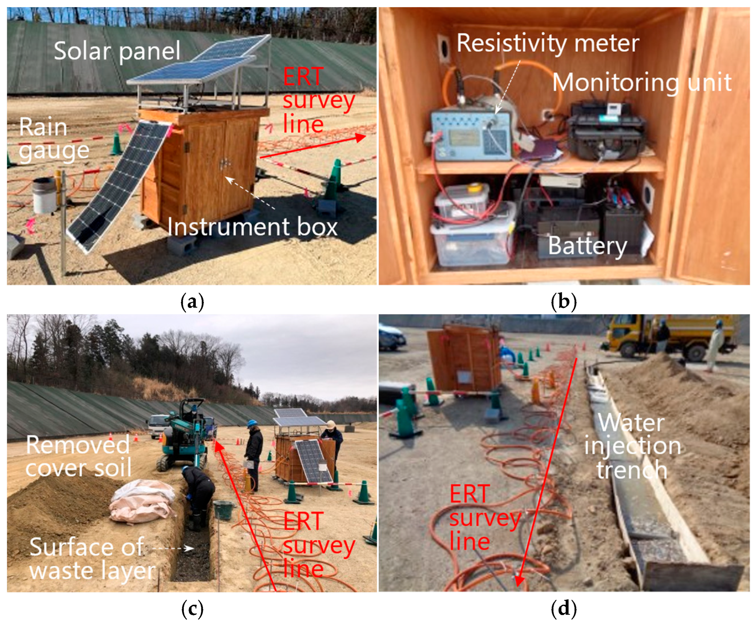
For the resistivity measurements, we used the ERT measurement system, which is a combination of a resistivity meter (Syscal Pro, IRIS Instruments, Orléans, France) and a remote-control unit (Syscal Monitoring Unit, IRIS Instruments), and performed all measurements remotely using an independent power supply consisting of a solar panel and lithium-ion battery.

The survey line of 23.5 m was established in a straight line on the ground surface of each landfill, and 48 stainless steel electrodes were driven in at 0.5 m intervals and connected to the instrument by a multicore coaxial cable. The measurement profile sequence was generated by the Electre II software (Version 05.06.00, IRIS Instruments), using the dipole–dipole method (a = 1, 2, 4 and n [depth level] = 1–14, 7–11, 21/4–26/4, respectively), and 872 raw data as an apparent resistivity were measured from the surface layer to a depth of approximately 4 m. The current injection time is 500 ms. The measurement time of each run is approximately 20 min.

Using the apparent resistivity data obtained from the measurements, we performed an inverse analysis using the finite element method and nonlinear least squares method to create a resistivity cross-section profile with the computer application of inversion (Res2DInv, Version 3.71, Aarhus Geo Software, Aarhus C, Denmark). Negative values and other anomalous values are removed from all data to ensure the quality of the dataset before analysis. The statistical algorithms of the resistivity data processing software (Prosys II, Version 03.13.06, IRIS Instruments) are used to automatically remove anomalous values. Specifically, finite element analysis is used to determine the distribution of resistivity from an initial model created with the measured potential data. The resistivity model is iteratively corrected using a nonlinear least squares algorithm to arrive at the resistivity profile.

2.2.2. Theoretical Background

Resistivity is a value that reflects various parameters in the ground, as indicated in Section 1. Soil resistivity is especially well-known as an effective indicator for understanding ground water flow and the physical and chemical properties of soil and waste, and it is known that the resistivity value mainly depends on the resistivity of pore water, the porosity, and the degree of saturation. These relationships are expressed as follows by Archie’s law [23], which is widely used as an empirical formula:

$$\rho =a\cdot {\rho }_w\cdot {\varphi }^{-m}\cdot S^{-n}$$

(1)

where $\rho$ is the apparent resistivity ($\Omega ·\mathrm{m}$), ${\rho }_w$ is the resistivity of pore water ($\Omega ·\mathrm{m}$), $\varphi$ is the porosity, $S$ is the degree of saturation, and $a$, $m$, and $n$ are experience constants. This formula provides the basic theoretical framework for relating changes in the resistivity distribution obtained by ERT to changes in subsurface water content and the progress of washout in landfills.

Since pore water conductivity and porosity are not considered to fluctuate rapidly during water injection tests or rainfall events, it is assumed that changes in saturation are primarily responsible for the decrease in resistivity.

2.2.3. Evaluation of Time-Dependent Resistivity Change

In order to quantitatively understand the change in resistivity over time and estimate the migration path of water within the landfill site (preferential flow path, or water channel), the resistivity change ratio ($\Delta \rho$) was calculated using the following formula [9]:

$$\Delta \rho ={\displaystyle \frac{{\rho }_n-{\rho }_{init}}{{\rho }_{init}}}\times 100$$

(2)

where ${\rho }_{init}$ is the resistivity before water injection or at the reference time ($\Omega ·\mathrm{m}$), ${\rho }_n$ is the resistivity after $n$-hours from water injection, and $\Delta \rho$ is the resistivity change ratio (%). Based on the cross-sectional distribution and histogram obtained from this calculation, it is possible to visually and quantitatively evaluate the depth and spread of water intrusion into the landfill site, the presence of water channels in specific areas, and the long-term stabilization process (washout progression).

2.3. Monitoring During Water Injection Test

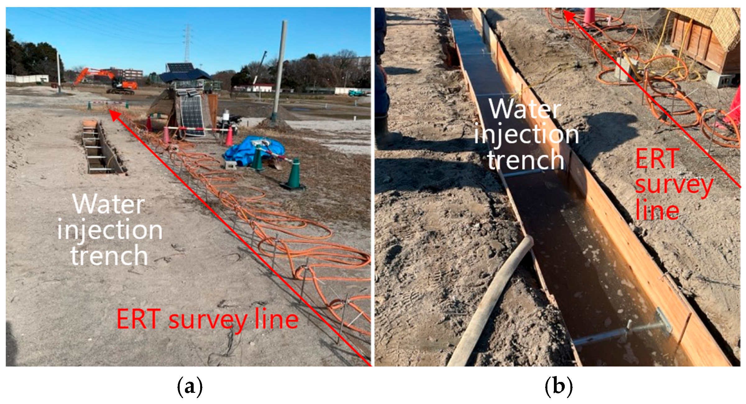
At both Site A (non-combustible waste landfill) and Site B (incineration ash landfill), water injection tests were conducted by excavating injection trenches of 0.6 m wide, 0.5 m deep, and 10 m long, and placing them 1 m away from and parallel to the ERT survey line (Figure 1 and Figure 2). Water infiltration was limited to the gravity direction by installing impermeable plates on the walls of the injection trenches.

Three injection tests were conducted at Site A. Water injection was performed by releasing water from a water truck into the excavation injection trench until the trench was filled with water. Water injection was performed three times, with each injection scheduled to begin approximately 72 h after the previous injection. Measurements were taken at approximately 20 min intervals and for a total of 66 ERT measurements, including the measurement prior to the first injection. Three injection tests were also conducted at Site B, and a total of 40 ERT measurements were taken. The behavior of water migration and the existence of water channels in the two landfill sites were estimated from the changes in resistivity after each injection.

2.4. X-Ray CT Scanning for Observating Pore Structure of Landfilled Waste

To verify whether the time-series changes in resistivity variation obtained from ERT represent the dynamics of water flow, undisturbed samples were obtained near the survey line and subjected to X-ray CT analysis to evaluate the three-dimensional pore structure.

It is rare and difficult to obtain undisturbed samples from waste layers in a landfill. We considered the management constraints of the landfill and our experience after consulting with civil engineering specialists and conducting preliminary test excavations. As a result, we decided to obtain undisturbed samples using the following procedures. (1) The size of the undisturbed sample was determined in advance, taking into account the specifications and measurement conditions of the X-ray CT analysis equipment described below. For this purpose, a trench with the dimensions W 1500 × D 3000 × H 1600 mm was excavated as a working area. (2) The sample container was pressed against the vertical surface of the exposed waste layer in the trench. The container was fixed with a pipe support and pushed while the waste around the container was manually dug up and removed. (3) After the sample container was fully inserted into the landfill layer, a cut was made along the rear edge of the container. (4) We lifted the sample container filled with landfill waste to the ground and used a cutter or pliers to flatten the surface. (5) The sample container filled with landfill waste was covered with a plate (lid) of the same material and secured with screws to prevent disturbance of the internal sample during transport. At this time, any large gaps on the surface or edges of the sample were filled with transparent construction adhesive as a sealant before closing the lid. (6) The sample container containing the landfill waste was transported to the X-ray CT analysis room. It was subjected to X-ray CT analysis in its original state. The sample containers were made of wood or polyvinyl chloride resin.

The reason for using this sampling method was that it has long been recognized that pushing the casing during drilling operations could potentially entangle surrounding debris. In addition, wood and vinyl chloride resin have low density and high X-ray permeability, which allows X-ray CT analysis of waste materials packed in sample containers several centimeters in size. Furthermore, both wood and vinyl chloride resin have excellent strength and elasticity; thus, they will not break even when the sample containers are pressed into the landfill layer.

The dimensions of the samples obtained were 240 mm width × 240 mm depth × 450 mm height at Site A and 80 mm width × 80 mm depth × 450 mm height at Site B. The collection containers were subjected to X-ray CT analysis using a large-scale inspection X-ray CT system C2 (manufactured by Nikon Corporation, Tokyo, Japan) with analysis conditions set at 450 kV using a µ-focus X-ray source. Priority was given to maximizing the imaging area for detailed examination of the extensive pore structure, resulting in a resolution of 0.146 mm. The upper and lower halves of the sample were imaged separately and then combined to construct a three-dimensional accurate pore structure as a single sample. VGSTUDIO MAX (Volume Graphics) was used as the CT image analysis software.

3. Results and Considerations

3.1. Results of Water Injection Test at Site A

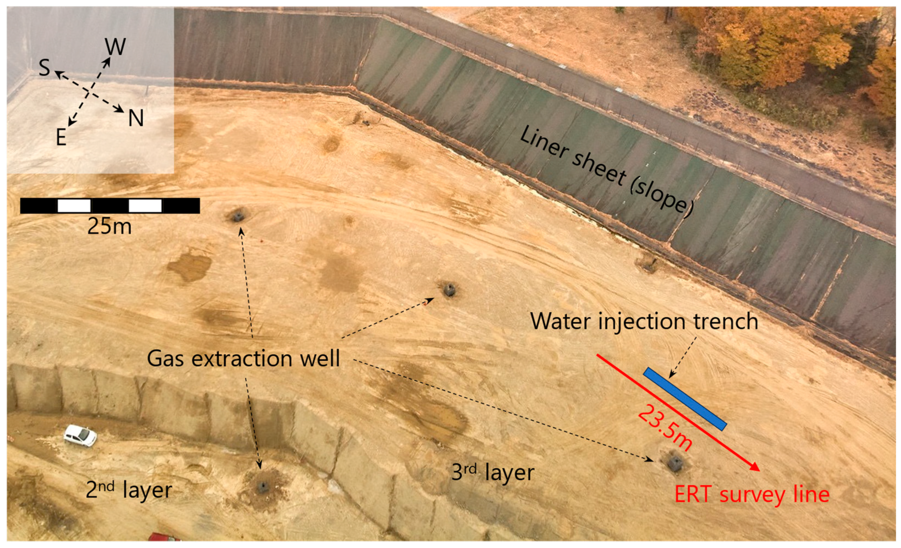
The layout of the ERT survey line and the water injection trench is shown in Figure 3. The water injection test at Site A was able to capture the time-dependent changes in resistivity structure caused by water injection using the 66 ERT monitoring sessions. The resistivity cross-sections before and 6 h after the first water injection test are shown as the change in resistivity before and after the water injection test (Figure 4). From the ground surface to a depth of 0.5 m, high resistivity of 100 $\Omega ·\mathrm{m}$ or higher was horizontally distributed (Figure 4a). This layer is the top cover soil layer above the waste layer, which is a gravel-mixed soil mined in the vicinity of Site A. A high resistivity area of 80 $\Omega ·\mathrm{m}$ was also distributed at depths below 3.5 m. The landfill structure of Site A suggests that this is due to the intermediate cover soil layer below the waste layer. On the other hand, the waste layer (0.5 to 3 m depth) sandwiched between the top and intermediate cover soil layers showed a heterogeneous resistivity distribution. In the 2 to 7 m and 8.5 to 13 m horizontal regions, the upper layers at depths of 0.5 to 1.5 m showed high resistivity of more than 100 $\Omega ·\mathrm{m}$, while the lower layers at depths of 1.5 to 3 m showed a significant decrease in resistivity to less than 30 $\Omega ·\mathrm{m}$. This means that the high water content in the deep layers has not changed even four years after the landfill was filled. Conversely, high resistivity of more than 150 $\Omega ·\mathrm{m}$ was dominant in the lower layers at depths of 1.5 to 3 m in the 16 to 18 m horizontal region.

Six hours after the first water injection test, the resistivity of the entire waste layer decreased significantly (Figure 4b). In particular, in the 7 to 8.5 m horizontal direction, the resistivity was over 50 $\Omega ·\mathrm{m}$ before water injection but decreased to 30 $\Omega ·\mathrm{m}$ after water injection. However, in the 13–18 m horizontal zone, the decrease in resistivity was less than in other areas. It was considered because of the presence of a gas ventilation pipe in the vicinity, about 3 m away from this region (Figure 3). Several vertical gas extraction wells consisting of a 200 mm diameter PVC pipe and a protective layer of quarry stone (1 m × 1 m) are installed in Site A. Since these gas extraction wells are connected to the collection and drainage pipes at the bottom of the landfill and also provide a drainage path for internal water, the pipes and protective layer have not only high porosity but also extremely low saturation, resulting in higher permeability and drainage than the waste layer. In addition, it is difficult for heavy equipment to compact the waste around the gas extraction well, and the porosity of the waste layer tends to be high. This suggests that in this area, injected water moved toward the gas extraction well and drained away, resulting in higher resistivity. These results indicate that the water entering from the injection trench moved heterogeneously in a subsurface direction and that multiple water channels exist in the waste layer. On the other hand, there was almost no decrease in resistivity in the surface cover soil layer during water injection. This is because both sides of the water injection trench were covered with impermeable panels, so that the injected water moved only in the vertical direction, and, thus, the moisture content in the intermediate soil cover layer did not increase.

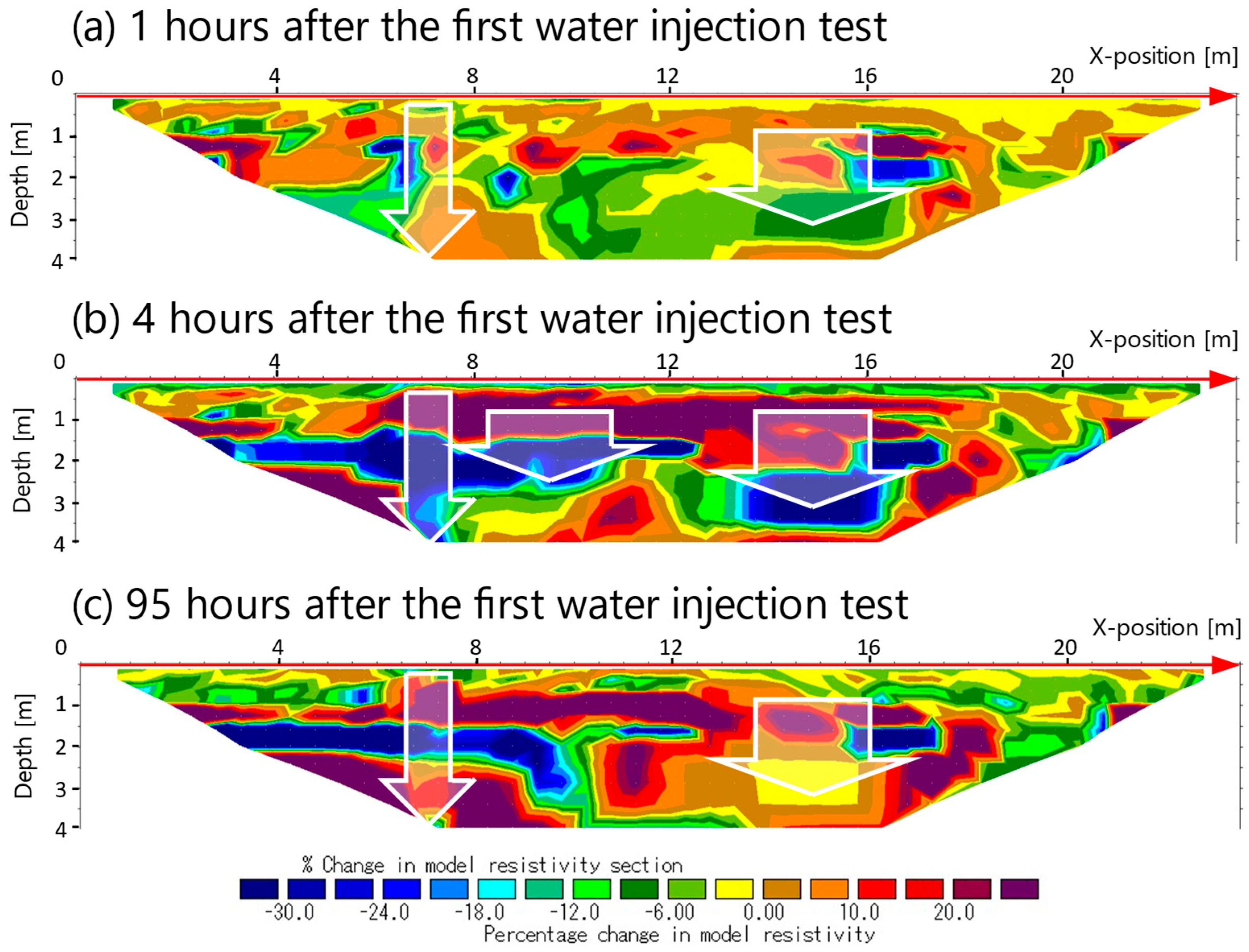
To quantitatively visualize the resistivity change, a cross-sectional distribution plot of the resistivity change rate ($\Delta \rho$) at 1, 4, and 95 h (Run 40, 45, and 65, respectively) after the third water injection test was obtained (Figure 5), with Run 38 immediately before the third water injection test as ${\rho }_{init}$. The $\Delta \rho$ at 1 h after the third water injection test (Run 40) was mostly distributed in the range of −10 to 10% (Figure 5a), while at 4 h (Run 45), a positive $\Delta \rho$ of 25% and a negative $\Delta \rho$ of −30% were observed in the surface layer at 1 m and below 1.5 m, respectively (Figure 5b). After 95 h (Run 65), the distribution of negative $\Delta \rho$ became smaller and showed a tendency to return to the situation before water injection (Figure 5c). The increase in negative $\Delta \rho$ indicates an increase in internal water content and a decrease in resistivity, indicating that the injected water moved from the surface to the subsurface, reaching a depth of 1.5 m or more after 4 h and then moving slowly with time. The numerical simulation results from Zhao et al. show that resistivity decreases with high sensitivity with water penetration into pore structures such as fractures [24]. And Henine et al. found that injecting high-pressure air into the ground increased the rate of resistivity change and identified a decrease in water content as a factor in this increase [25]. These previous studies support the results of this study in that a sudden change in ground water content can affect resistivity change. The high-resistivity region near the gas extraction well mentioned above and the three regions circled by the white dotted lines in Figure 5 showed particularly large changes in $\Delta \rho$, suggesting the possible existence of water channels in these areas. Dumont et al. also suggested that gas wells were affecting the vertical water flow in landfill using ERT monitoring [26]. These ERT monitoring results not only identified the extensive downward migration of water content from the water injection test but also strongly suggested that multiple water channels were unevenly distributed as prominent migration pathways in the waste layer where non-combustible residues were landfilled.

3.2. Results of Water Injection Test at Site B

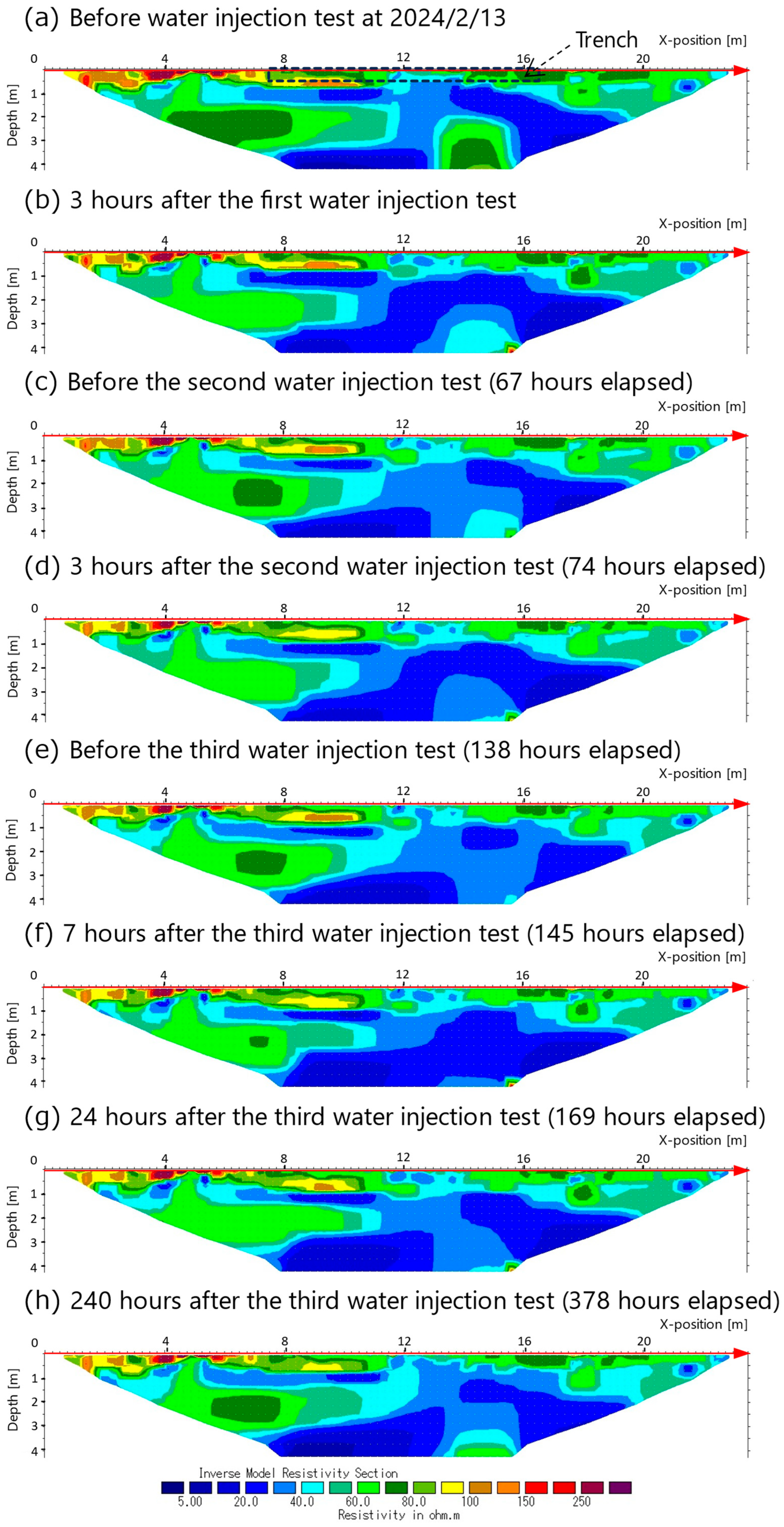
Figure 6 shows the measured resistivity distributions before and after the water injection test at Site B. Before the water injection test, the overall resistivity at Site B was lower than at Site A (Figure 6a). The main components of waste are inert, non-combustible residue at Site A, and incineration ash at Site B, as mentioned in Section 2.1. Thus, it was considered that the large amount of soluble chemicals such as salt and water content remained high at Site B even after 7 years of landfilling and the progress of washout was still limited compared to Site A. Additionally, the water infiltration rate during the initial water injection test was 3.10 cm/min at Site A and 0.77 cm/min at Site B. This indicates that Site B, which only accepts incineration residue, has not only higher salinity but also lower permeability and slower washout conditions than Site A, which only accepts non-combustible residues.

The resistivity structure before water injection shows that, although there was no soil cover layer as in Site A, resistivity regions of 15 $\Omega ·\mathrm{m}$ or higher were distributed horizontally from the ground surface to a depth of 1 m. Below 1 m, very low-resistivity regions of 5 $\Omega ·\mathrm{m}$ or lower were widely distributed, especially in the 12 to 20 m horizontal direction (Figure 6a). No significant change in resistivity was observed in the surface layer at a depth of 0.5 m from the ground surface as a result of the water injection test. As in Site A, this is thought to be due to the fact that the water injection test did not affect the change in water content at the soil surface due to the structure of the injection trench. It is clear that the positioning of the survey line installation and the adjustment of the exploration depth in the ERT measurements have a significant impact on the analytical resolution. Three hours after the first water injection, a significant decrease in resistivity was observed at depths greater than 1 m in the 7–17 m horizontal area where the injection trench was located (Figure 6b). And 67 h later, prior to the second water injection test, resistivity increased and showed a tendency to approach the pre-water injection resistivity structure (Figure 6c). These resistivity changes were particularly pronounced in the region from 11 m to 16 m horizontally and from 1.5 m to 4 m in depth. Visual inspection of infiltration during water injection also showed a tendency for faster infiltration in the area between 12 and 17 m of the trench, indicating that the amount of infiltrating water moving in this area was large and that it may have become a water channel. While maintaining a lower resistivity than before water injection, the second and third water injection tests also showed a similar trend of a decrease in resistivity immediately after water injection and a gradual increase thereafter (Figure 6d–g), returning to the same resistivity distribution as before water injection after 240 h (Figure 6h).

These results indicate that water movement can be visualized even at Site B, and that ERT monitoring is an effective method for detecting and visualizing water channels non-destructively, regardless of differences in landfill waste type and landfill age.

3.3. Pore Structure of Landfilled Waste

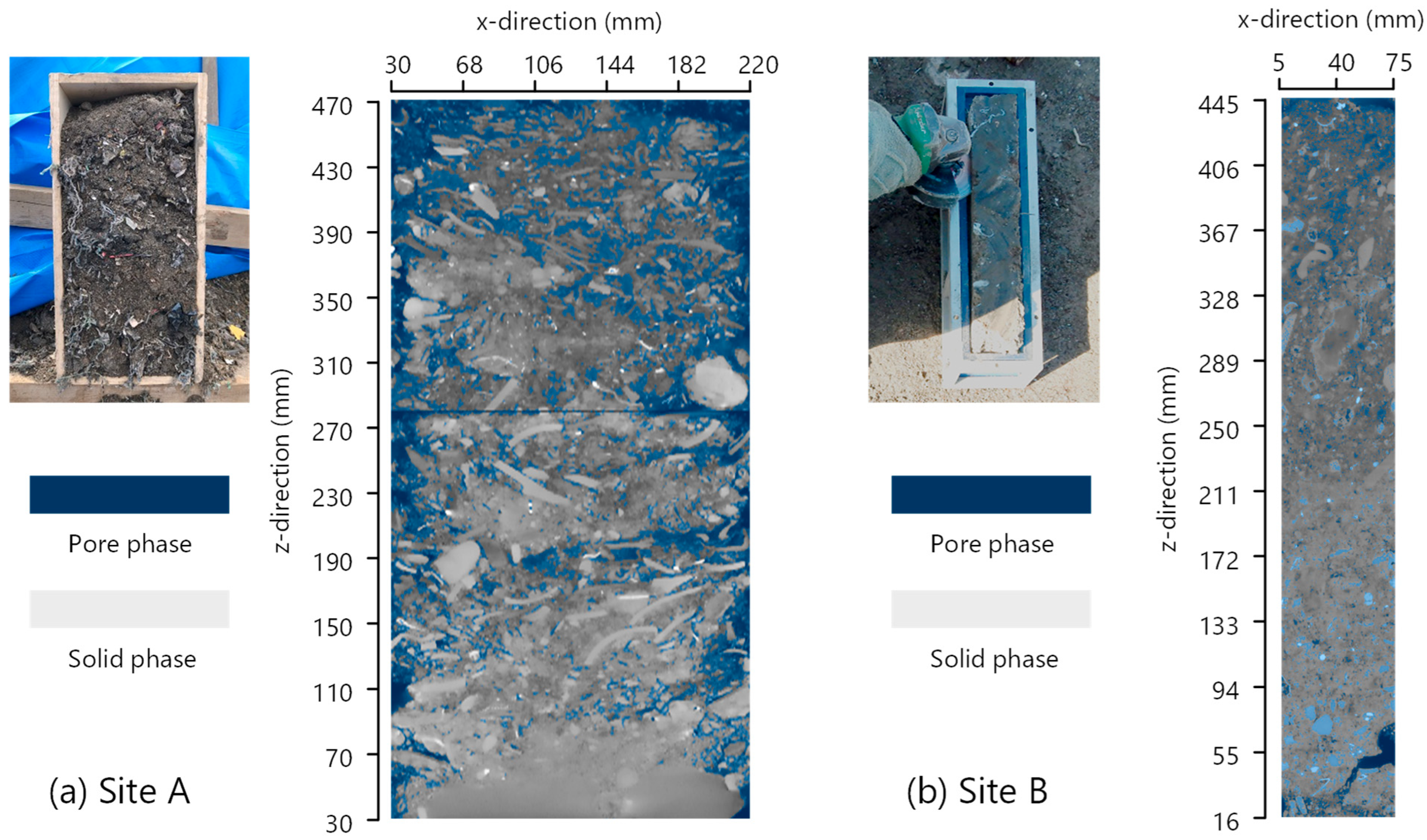
Figure 7 shows cross-sectional images and X-ray CT analysis results for the waste samples from Site A and Site B. Visually, the samples collected from Site A contained incineration ash, non-combustible materials, and plastic waste, with numerous fine fibers observed in some areas. Samples from site B were primarily incineration ash but had a significant amount of metal fragments. The incineration ash had solidified, making it difficult to cut even with a motorized cutter. Therefore, the sample from Site B became smaller than that from Site A.

At Site A, where non-combustible residues are the main component of the landfill waste, various materials such as fibers, plastics, incineration ash, and metals existed in the pores. In contrast, at site B, where incineration residues are the main component of the landfill waste, the pores were scattered compared to Site A, indicating a more compact porous medium.

Three-dimensional image data obtained through X-ray CT analysis can be used to quantitatively evaluate the porosity and tortuosity of a porous structure in waste. First, image processing was applied to the acquired CT images. Thresholding was performed to binarize the solid and void regions. The ratio of void pixels to total pixels on a horizontal slice of the binary images was calculated to determine porosity.

Next, tortuosity is evaluated by calculating the ratio of the geometric length of the flow path within the pore network to the straight-line distance. The flow path can be estimated using the fluid analysis of the porous structure. Thus, the geometric length of the flow path is determined by producing the flow vector and time step. On the other hand, the straight-line distance can be obtained by projecting the flow vector onto the depth vector. The tortuosity of the fluid flow path is quantified by dividing the geometric length of the flow path by the straight-line distance from the starting point of the flow to the endpoint.

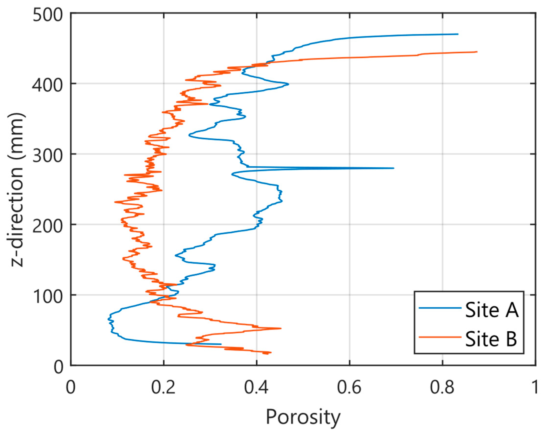
Figure 8 shows the distribution of void ratio in the depth direction. In the non-combustible residue landfill layer, the average value was 0.328, but it decreased with increasing depth. In the incineration ash landfill layer, the average value was 0.195. The incineration ash at Site B was landfilled at least 7 years ago and had solidified naturally, resulting in low porosity. No change in porosity with depth was observed in the incineration ash landfill layer.

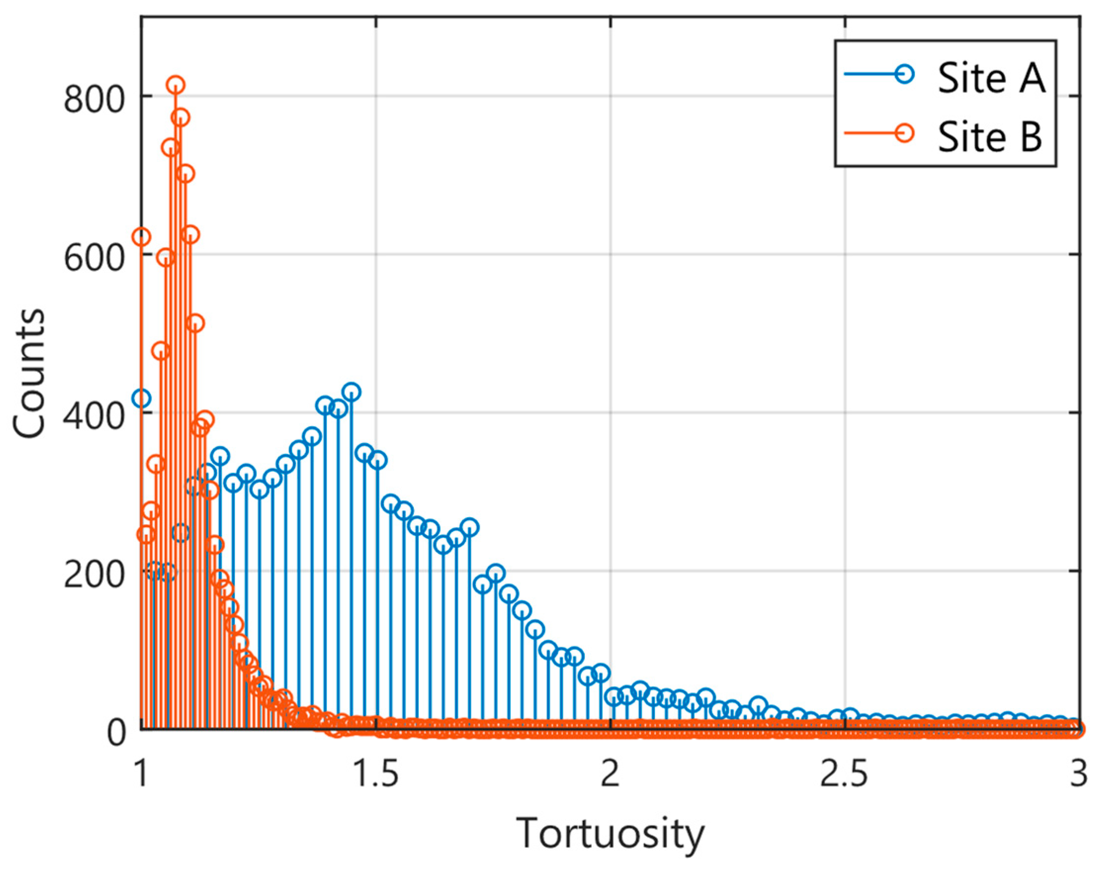
Figure 9 shows the tortuosity histogram. Tortuosity is an indicator of the meandering nature of flow paths, with higher values indicating greater meandering. The tortuosity of the incineration ash landfill layer had a sharp histogram with a peak value of 1.07, while the non-combustible residue landfill layer had a broad histogram with a peak value of 1.44. When comparing the tortuosity of non-combustible residues and incinerated ash, significant differences were observed, suggesting that tortuosity could serve as one of the indicators for assessing the presence of water pathways.

Casado et al. reported that low resistivity values were detected in areas with dense fault planes, suggesting that these areas serve as pathways for seepage water [16]. This supports the idea that areas of relatively high porosity may act as water pathways. Site A had higher resistivity values overall, despite the shorter time elapsed since landfill closure compared to Site B. It suggests that this difference is due to not only variations in the quality of the landfill waste, but also progress in pollutant washout by rainwater infiltration. A pore structure with high porosity, such as at Site A, where non-combustible wastes are landfilled, will cause water channel flow that enhances the washout effect along the path.

3.4. Further Study

The resistivity obtained by ERT is a site-specific value that comprehensively reflects the physicochemical properties inside the landfill and the type of landfill waste, as expressed in Archie’s law, and, thus, has limitations that make it inapplicable for interpretation at other sites. As a future development of ERT monitoring, the effectiveness of ERT monitoring in unknown landfill sites is expected to increase when combined with AI-driven networks. The use of AI in the inverse analysis process is expected not only to increase the resolution and inference speed of geophysical surveys but also to detect the features and trends related to time-dependent physics [27,28]. The time-lapse ERT used in this study is also consistent with the slope stability assessment [28]. Using a similar approach, such as Sen’s slope estimator, suggests that time-lapse ERT will effectively detect water infiltration paths and estimate the time required to wash out pollutants. Since resistivity electrical survey is widely used as a leak detection system for waste disposal sites in Japan, the utilization of AI and ERT is expected to reduce costs by using fewer electrodes, shortening data acquisition time, and understanding real-time impervious performance [29].

4. Conclusions

In this study, we attempted to visualize the behavior of water migration in the waste layer during water injection tests using ERT monitoring at Site A, which is mainly composed of non-combustible residues, and Site B, which is mainly composed of incineration ash. The main results obtained are as follows.

• Electrical resistivity tomography (ERT) was used to capture the changes in the two-dimensional and time-series distribution of water migration in the landfill, and it was possible to detect the existence of water channels and the dynamics of saturated regions that could not be captured by point methods.
• Water injection test monitoring clearly captured the large-scale vertical migration of water in the waste layer and the behavior of unevenly distributed water channels. The water infiltration rate was 3.10 cm/min at the landfill site containing mainly non-combustible residues and 0.77 cm/min at the landfill site containing only incineration residue.
• X-ray CT analysis of undisturbed samples revealed differences in pore structure depending on the type of waste landfilled. The porosity of the landfill layer composed mainly of non-combustible residues was 0.328, while the porosity of the landfill layer composed of incineration ash was 0.195. Since incineration residue is easier to compact than non-combustible residues, its porosity is smaller and its water permeability rate is lower. The results of the X-ray CT analysis were consistent with the infiltration rate measured in the injection test.
• Analysis of the change in resistivity has been shown to be effective not only as an indicator of changes in water content but also as an indicator of changes in the electrical conductivity of pore water due to washout (i.e., the progression of landfill stabilization). In landfills composed mainly of incineration ash, the salt in the ash is flushed. This results in significant changes in resistivity and makes it easier to capture the washout process with ERT.
• It was confirmed that the characteristics and structural differences of the landfill (e.g., the presence or absence of a final cover, layout of gas extraction wells, etc.) have a significant effect on the water migration behavior and the resistivity structure. This will be an important factor to consider in the design and maintenance of future landfills.