Deep Learning for Glioblastoma Multiforme Detection from MRI: A Statistical Analysis for Demographic Bias

Abstract

Glioblastoma, IDH-wildtype (GBM), is the most aggressive and complex brain tumour classified by the World Health Organization (WHO), characterised by high mortality rates and diagnostic limitations inherent to invasive conventional procedures. Early detection is essential for improving patient outcomes, underscoring the need for non-invasive diagnostic tools. This study presents a convolutional neural network (CNN) specifically optimised for GBM detection from T1-weighted magnetic resonance imaging (MRI), with systematic evaluations of layer depth, activation functions, and hyperparameters. The model was trained on the RSNA-MICCAI data set and externally validated on the Erasmus Glioma Database (EGD), which includes gliomas of various grades and preserves cranial structures, unlike the skull-stripped RSNA-MICCAI images. This morphological discrepancy demonstrates the generalisation capacity of the model across anatomical and acquisition differences, achieving an F1-score of 0.88. Furthermore, statistical tests, such as Shapiro–Wilk, Mann–Whitney U, and Chi-square, confirmed the absence of demographic bias in model predictions, based on p-values, confidence intervals, and statistical power analyses supporting its demographic fairness. The proposed model achieved an area under the curve–receiver operating characteristic (AUC-ROC) of 0.63 on the RSNA-MICCAI test set, surpassing all prior results submitted to the BraTS 2021 challenge, and establishing a reliable and generalisable approach for non-invasive GBM detection.

1. Introduction

Glioblastoma, IDH-wildtype (GBM), classified by the World Health Organization (WHO) as a grade IV glioma [1], represents the most aggressive and prevalent primary malignant brain tumour in adults, accounting for approximately 60% of such cases [2]. The estimated annual incidence of glioblastoma in the United States is 3.26 cases per 100,000 individuals, with age-specific rates increasing progressively: 0.15 in children (0–14 years), 0.58 in adolescents and young adults (15–39), 7.03 in adults over 40, and reaching 15 in the 75–84 age group [3]. Early detection and conventional treatments for GBM have demonstrated limited efficacy, primarily due to its invasive nature and the restrictive properties of the blood–brain barrier [4]. Despite multimodal therapeutic advances, including surgery, radiation, and chemotherapy, the median overall survival remains between 12 and 15 months post-diagnosis, and the 5-year survival rate is only 6.9% [2,3,5]. These figures highlight the limitations of standard diagnostics approaches, underscoring the risk of complications and the associated high costs, while emphasising the urgent need for improved diagnostic support systems [6].

Despite being the current diagnostic gold standard, histopathological confirmation of GBM through invasive procedures, such as stereotactic biopsy or surgical resection, presents significant clinical challenges [7]. These methods carry substantial risks, including surgical morbidity (haemorrhage, infection, and neurological deficits), and they typically require prolonged hospitalisation [8]. Furthermore, the intrinsic spatial heterogeneity of GBM tumours often leads to sampling bias during biopsy, compromising diagnostic accuracy and limiting the reproducibility of the technique [9]. This biological constraint, coupled with procedural risks, significantly hinders effective longitudinal monitoring of tumour progression and treatment response. This underlines the need to develop safer and non-invasive diagnostic tools, particularly for patients in advanced stages of the disease [10].

Magnetic resonance imaging (MRI) has emerged as a crucial and non-invasive technique for the diagnosis of GBM, offering precise details on tumour morphology and demonstrating its value in neuro-oncology [11,12]. In addition to its application in GBM diagnosis, MRI has been widely used to characterise various other cancers, including gastric, lung, and colon cancer, proving its versatility and diagnostic value [13,14,15]. Furthermore, MRI contributes to increased diagnostic precision and safety, particularly when incorporated with deep learning techniques [16] to improve the detection of cervical cancer [17].

The integration of deep learning into the medical field has led to significant advances by improving the detection and treatment of brain tumours, including GBM [18]. Deep learning methods have shown encouraging results in a range of computer vision tasks, including segmentation, classification, and object detection [11,19,20]. These methods employ convolutional layers capable of extracting a hierarchical spectrum of features from input images, ranging from low-level local features to high-level global representations. In the final stage, a fully connected layer processes the extracted feature maps, transforming them into probabilistic predictions associated with specific labels [19]. However, achieving robust and reliable performance requires the careful design of optimal layer architectures, along with the meticulous fine-tuning of hyperparameters to enhance accuracy and generalisation capabilities [11,19].

To advance the frontier of medical imaging, the Radiological Society of North America (RSNA) and the Medical Image Computing and Computer-Assisted Intervention (MICCAI) have curated a detailed data set, hosted on Kaggle, featuring 585 patients [21]. This data set was used in the Brain Tumor classification (BraTS) 2021 challenge and includes information on the Weighted signal T1 (T1w), which provides anatomical details of brain tissue and facilitates the differentiation between grey and white matter. In addition, Kaggle provides a subset of 87 patients without associated diagnoses, which is employed as a test set for evaluating the developed model. The predictions generated via the model are submitted to Kaggle, which quantitatively assesses their classification performance by computing the area under the receiver operating characteristic curve (AUC-ROC). Subsequently, the evaluation results are returned to facilitate further analysis and the refinement of the model. This procedure privately evaluates the generalisation of the model using this specific data set [22]. Likewise, the Erasmus Glioma Database (EGD), curated by the Erasmus Medical Center (University Medical Center Rotterdam), provides a collection of 774 patients diagnosed with glioma, including T1w imaging data and demographic information, such as age and sex [23]. The EGD data set is used primarily for the development and validation of machine learning algorithms aimed at the classification, segmentation, and prognostic assessment of gliomas from grades I to IV. Each data set plays a role in advancing medical imaging research and enhancing clinical decision-support systems.

Machine learning algorithms can inadvertently learn and replicate patterns from training data that reflect demographic imbalances, such as disparities related to age or sex [24]. To examine whether such biases are present, demographic fairness is evaluated using statistical techniques, including the Shapiro–Wilk test for assessing normality, the Mann–Whitney U test for comparing age subgroups, and the Chi-squared test for associations based on sex [25]. By incorporating power analysis and confidence interval estimation, the analysis also provides insights into the robustness of performance metrics and supports a methodological framework for assessing demographic invariance [26].

In this study, a CNN-based model was developed using a data set provided by RSNA and MICCAI. This model was trained with the objective of comparing its performance with that of other researchers who also used this database. Subsequently, inference was conducted using the EGD database, demonstrating the ability of the model to generalise in detecting other types of gliomas using F1-score, accuracy, and a false negative rate. Furthermore, a statistical analysis was performed on the demographic information available in the new data set to investigate whether the model exhibited significant bias as a function of patient age or sex.

2. Materials and Methods

2.1. Data Set

2.1.1. Training Data Set

The RSNA and MICCAI developed a data set named the RSNA-MICCAI brain tumour radiogenomic classification for the BraTS 2021 challenge [21], which is available to the public through the Kaggle platform. This data set comprises multi-parametric magnetic resonance imaging (mpMRI) scans acquired from multi-institutional benchmarks, retrospectively collected for the prediction of a specific genetic characteristic of GBM, namely, the MGMT promoter methylation status, fulfilling strict inclusion criteria for image quality and diagnostic confirmation. An mpMRI scan typically includes four imaging modalities, each contributing distinct contrast mechanisms that facilitate tumour characterisation. In this study, only T1w images were selected for analysis (Figure 1), as this sequence provides the most morphologically informative signal [27]. All images were standardised to a resolution of 512 × 512 pixels to guarantee uniformity between analyses.

The BraTS 2021 challenge employs AUC-ROC as its primary evaluation metric, providing a framework for assessing model performance in GBM classification tasks [21]. The ROC curve is a widely utilised tool for evaluating the effectiveness of binary classification models by plotting the true positive rate (sensitivity) against the false positive rate (1—specificity) across various decision thresholds. This graphical representation provides information on the ability of the model to distinguish between classes, independent of a particular threshold. The AUC, derived from the ROC curve, offers a comprehensive summary of the performance of the classifier by quantifying the overall discriminatory power as a single scalar value ranging from 0 to 1. An AUC value of 0.5 indicates random performance, whereas values closer to 1.0 signify superior classification capabilities [28]. The principal benefit of AUC is its validity in the context of unbalanced data sets [29].

In accordance with the machine learning paradigm of algorithmic evaluation, the BraTS 2021 challenge data is divided into training and testing data sets [21]. The training data set contains complete mpMRI data from 585 patients, with a primary analytical focus on the T1w sequences. In contrast, the testing data set consists of 87 patients and maintains fully blinded diagnostic labels through the Kaggle evaluation platform, ensuring an unbiased assessment of model generalisability. Participants submit predictions for the test set through this private evaluation system, which automatically calculates AUC-ROC metrics as the primary performance benchmark.

All cases were evaluated by a panel consisting of four board-certified neuroradiologists, with binary classification labels (“0” indicating negative and “1” indicating positive for GBM) assigned through consensus review [30]. This validation process ensures diagnostic reliability, while the structure of the data set maintains a rigorous separation between training and evaluation data, preventing information leakage during model assessment. The main characteristics of this data set are outlined in

Table 1. Key characteristics of the RSNA-MICCAI BraTS 2021 data set.

Field	RSNA-MICCAI BraTS 2021
Patients	672
Demographic data	Not available in the public release
Scanner (Tesla)	Multicenter scanners (mainly 1.5T and 3T)
Data format	MRI in DICOM and NIfTI formats
Total size	142 GB
Origin	Multiple international institutions
Acquisition years	Up to 2014–2020 (preoperative scans)
Imaging modalities	Native T1, contrast-enhanced T1, T2, T2-FLAIR
Access	Public (CC-BY license, registration via TCIA)

.

2.1.2. Inference Data Set

EGD is a valuable resource for neuro-oncology research, representing one of the most comprehensive multicenter collections. It contains preoperative curated T1w magnetic resonance images (Figure 2), molecular biomarkers, and tumour segmentations from 774 patients with glioma treated at Erasmus Medical Center (University Medical Center Rotterdam) between 2008 and 2018.

Patient demographic data include 281 women, 492 men, and one patient of unspecified sex. The age distribution ranges from 19 to 86 years. However, 49 patients with age records marked with the −1 label were identified, indicating missing information. Among them, one patient had neither age nor sex data available [23]. This data set differs significantly from RSNA-MICCAI in terms of anatomical presentation, as the T1w images in EGD retain full cranial anatomy, whereas the training set consists of skull-stripped images. This contrast enables the assessment of the model’s ability to generalise across differing acquisition and preprocessing protocols. A summary of the data set characteristics is provided in

Table 2. Key characteristics of the Erasmus Glioma Database.

Field	Erasmus Glioma Database (EGD)
Patients	774 glioma cases (281 female, 492 male, 1 unknown)
Demographic data	Available (age and sex)
Scanner (Tesla)	Siemens, Philips, GE, Toshiba: 1.5T (571), 3T (83), 1T (110), 0.5T (6)
Data format	NIfTI (registered to MNI atlas, skull-stripped)
Total size	101 GB
Origin	Erasmus MC, Rotterdam, The Netherlands
Acquisition years	2008–2018 (preoperative scans)
Imaging modalities	Native T1, contrast-enhanced T1, T2, T2-FLAIR
Access	Restricted

.

To ensure consistency, the same predictive task identifying imaging features associated with GBM—was applied across both data sets. Although the RSNA-MICCAI data set was originally designed for radiogenomic classification based on MGMT promoter methylation, the analysis instead focused on detecting characteristic GBM visual patterns. In the case of the EGD data set, the model was evaluated by identifying cases consistent with WHO grade IV glioblastoma. Despite differences in labelling criteria and image preprocessing particularly the use of skull-stripped images in RSNA-MICCAI versus full head scans in EGD both data sets are clinically aligned with GBM detection. These variations introduced valuable diversity in the input data, allowing a rigorous assessment of the model’s ability to generalise across different anatomical and acquisition settings.

2.2. CNN Architecture and Training

The CNN model was trained using the RSNA-MICCAI data set provided for the BraTS 2021 challenge [21]. In this phase, a sequential experiment was conducted by adjusting the number of neurons and layers in the CNN architecture to identify the configuration demonstrating superior performance A hyperparameter tuning analysis was subsequently performed on the selected model.

All proposed layer configurations were evaluated through an iterative and automated process. For each configuration, a specific model was constructed and compiled with the Adam optimiser and a binary cross-entropy loss function. The entire data set, comprising 585 patients, was subjected to 5-k-fold cross-validation strategy, ensuring robust/reliable performance estimation and avoiding overfitting. Fixed parameters across all models included a learning rate of 1 × 10⁻³, batch size of 64, and 200 training epochs with early stopping after 120 epochs, using 5-fold cross-validation. The final model included 98,384 trainable parameters, occupying 384 KB in 32-bit precision.

As depicted in Figure 3, the trained model was subsequently validated using EGD to assess its generalisation performance. This validation step allowed for a thorough evaluation of the model in different types of glioma.

2.3. Inference

Statistical Tests

To ensure the reliability and fairness of the model, statistical tests were conducted, starting by implementing the Shapiro–Wilk test to assess whether the data sample followed a normal distribution. This was necessary to determine the application of parametric or non-parametric tests.

$$W={\displaystyle \frac{{\left({\sum }_{i=1}^n{a}_i{x}_{\left(i\right)}\right)}^2}{{\sum }_{i=1}^n{(x_i-\overline{x})}^2}},$$

(1)

In Equation (1), $x_{\left(i\right)}$ represents the ordered observations, $a_i$ refers to the constants derived from the means, variances, and covariances of the normals, and $\overline{x}$ denotes the mean of the sample. The Shapiro–Wilk test is commonly used in medical research and statistical evaluations, as seen in the analysis of automated algorithms for the detection of small bowel tumours [31]. The test was applied to assess the normality of two statistical features (skewness and kurtosis), used to differentiate tumorous and non-tumorous frames, followed by the use of non-parametric methods for classification.

For group comparisons across two independent groups, the Mann–Whitney U test was applied to assess whether there was a statistically significant difference in their distributions.

$$U=n_1{n}_2+{\displaystyle \frac{n_1(n_1+1)}{2}}-R_1,$$

(2)

In Equation (2), $n_1$ and $n_2$ refer to the sample sizes of the two groups, and $R_1$ represents the sum of the ranks of the first sample. The Mann–Whitney U test is often used to evaluate the significance of differences in non-normally distributed data, particularly when dealing with medical data sets, as seen in radiomic-based studies for cancer prediction [32]. These studies implemented this test to assess the relationship between clinical variables on the ordinal scale and invasive disease-free survival (iDFS) for breast cancer patients, incorporating the results into a stratified feature selection pipeline.

Complementing these analyses, the Chi-square test was used to examine the existence of a significant relationship between two categorical variables.

$${\chi }^2=\sum {\displaystyle \frac{{(O_i-E_i)}^2}{E_i}},$$

(3)

In Equation (3), $O_i$ denotes the observed frequencies in each category and $E_i$ represents the expected frequencies for these categories, assuming the independence of the variables. The Chi-square test is used in biomedical applications to assess relationships, as demonstrated in ensemble classifiers for biomedical data [33]. Therefore, this test was applied in a preliminary step as a filter feature selection method to evaluate the relevance of each attribute concerning class labels in multiple medical data sets.

In statistical hypothesis testing, the null hypothesis ($H_0$) assumes the absence of association between studied variables, representing a baseline state. Conversely, the alternative hypothesis ($H_1$) posits a significant effect or difference [34]. The sampling distribution of the test statistic, defined under $H_0$, enables the assessment of whether observed data provide sufficient evidence to reject $H_0$ in favour of the $H_1$. These hypotheses guide the statistical tests applied in this study.

The statistical analysis was conducted in three steps. Firstly, the Shapiro–Wilk test (Equation (1)) was performed to assess whether the age distributions in the FN and TP groups were normal. Secondly, the Mann–Whitney U test (Equation (2)) evaluated differences in age distributions across prediction outcome groups within age cohorts. Finally, the Chi-squared test (Equation (3)) was applied to evaluate the relationship between sex and the correctness of the predictions of the model. All analyses were performed using a two-tailed significance level of 0.05, a conventional threshold in hypothesis testing to control the probability of Type I error, since one in twenty (0.05) chances represents an unusual sampling event [35]. Statistically, this implies a 5% probability of falsely rejecting the null hypothesis; consequently, p-values above this threshold indicate insufficient evidence to reject it.

In addition to significance testing, Confidence Intervals (CIs) were considered to quantify the precision of estimated parameters by providing a range over which the true value is expected to lie with a given probability. Unlike p-values, CIs convey both the magnitude and direction of effects [36]. In this study, a 95% confidence level was applied, corresponding to the 0.05 significance threshold defined. The 95% CI for a sample mean was calculated as

$${\mathrm{CI}}_{95\%}=\overline{x}\pm z·{\displaystyle \frac{\sigma }{\sqrt{n}}},z=1.96,$$

(4)

where $\overline{x}$ denotes the sample mean, $\sigma$ the standard deviation, n the sample size, and z the z-score corresponding to the desired confidence level (1.96 for 95%) [36].

Additionally, to assess the sensitivity of each statistical test, a power analysis was conducted. Statistical power refers to the probability of correctly rejecting a false null hypothesis and, therefore, reflects the sensitivity of a test to detect true effects. It is mathematically defined as $1-\beta$, where $\beta$ is the probability of committing a Type II error (failing to reject the null hypothesis when it is false).

To determine the power for each test, specific alternative hypotheses were defined, tailored to the observed data and reflecting plausible deviations from the null hypothesis. For the Shapiro–Wilk test, the power analysis assumed an exponential distribution as an alternative hypothesis, as it is a plausible deviation from normality for age data in medical contexts and is commonly used in normality test evaluations [37]. For the Mann–Whitney U test, the power analysis assumed a shift in medians as the alternative hypothesis, given its relevance as a plausible deviation in age distributions within predictive modelling contexts [38]. For the Chi-squared test, the power analysis assumed a small effect size (Cohen’s w = 0.1), as it reflects a subtle yet meaningful departure from independence in categorical data analyses [25]. Power was assessed as the proportion of tests rejecting $H_0$ when using 10,000 simulations, corresponding to Monte Carlo simulation.

By incorporating these statistical methods, potential biases related to demographic factors were thoroughly examined, contributing to a more rigorous evaluation of CNN diagnosis precision in the detection of GBM.

2.4. Evaluation Metrics

The AUC-ROC metric was utilised to assess the accuracy of the proposed method. The evaluation of the model performance on the input images is based on classification measures, including true positives (TPs), true negatives (TNs), false positives (FPs), and false negatives (FNs). TP represents correctly identified positive cases, TN corresponds to correctly identified negative cases, FP refers to negative cases incorrectly classified as positive, and FN indicates positive cases incorrectly classified as negative. Based on these measures, a range of performance metrics may be derived. One of them is accuracy, which measures the overall correctness of the model, mathematically expressed as follows:

$$\mathrm{Accuracy}={\displaystyle \frac{TP+TN}{TP+TN+FP+FN}},$$

(5)

Although accuracy provides a general measure of performance, it may be inadequate for imbalanced data sets. To address this, precision and recall are often employed. Precision quantifies the proportion of true positive predictions among all cases predicted as positive, formally defined as follows:

$$\mathrm{Precision}={\displaystyle \frac{TP}{TP+FP}},$$

(6)

Conversely, recall (or sensitivity) measures the proportion of actual positives that were correctly identified, represented as follows:

$$\mathrm{Recall}={\displaystyle \frac{TP}{TP+FN}},$$

(7)

These two metrics are typically combined into the F1-score, which is the harmonic mean of precision and recall, offering a balanced evaluation of the model, mathematically expressed as follows:

$$\mathrm{F}1\text{-}\mathrm{Score}={\displaystyle \frac{2·(\mathrm{Precision}·\mathrm{Recall})}{\mathrm{Precision}+\mathrm{Recall}}}$$

(8)

Furthermore, the false negative rate (FNR) is employed in contexts where missing positive cases is critical, such as the actual medical context. FNR is defined as:

$$\mathrm{False}\mathrm{Negative}\mathrm{Rate}={\displaystyle \frac{FN}{TP+FN}},$$

(9)

The experiments were conducted on a computing cluster equipped with two Nvidia T4 GPU units, each with 15 GB of memory (a total of 30 GB for GPU processing), supported with 29 GB of system RAM and a Ryzen 7 5700X 8-core processor at 3.40 GHz, along with 73.1 GB of disk storage.

3. Results

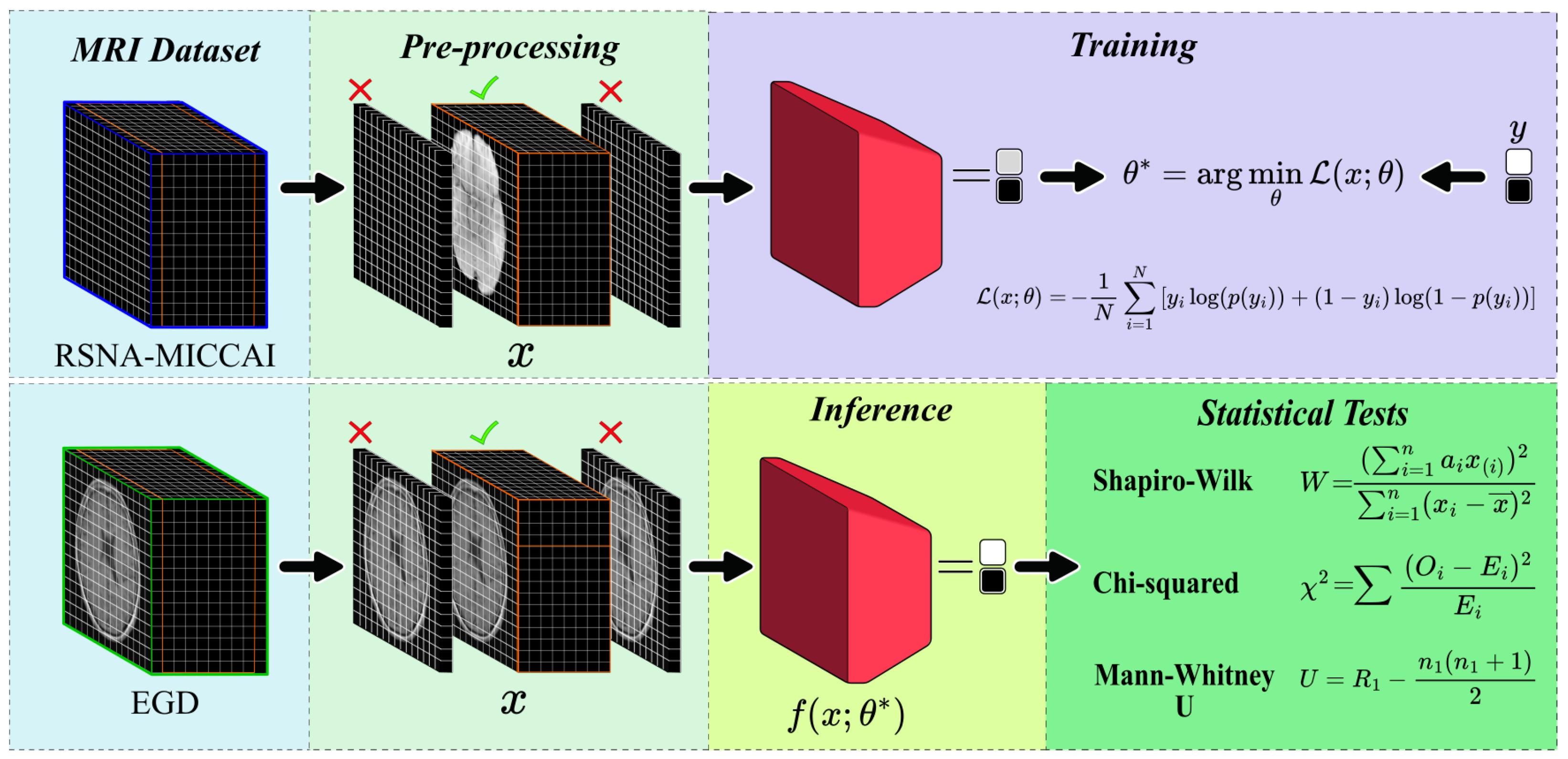
3.1. Training of the CNN Model for GBM Detection

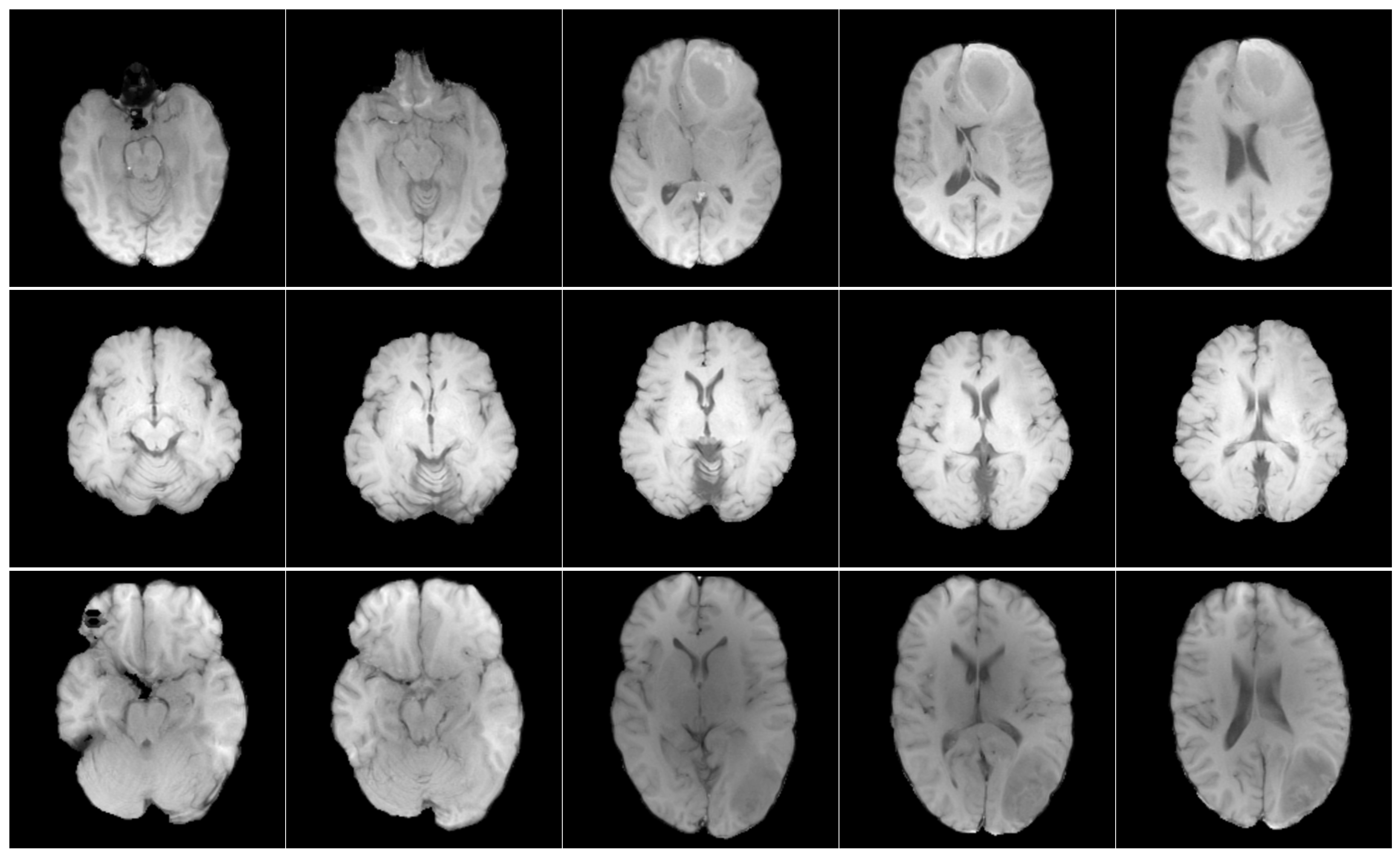
In the RSNA-MICCAI data set, all patient MRI scans were analysed. It was determined that 27.7% did not contain useful diagnostic information, specifically completely black. Consequently, 72.3% of the remaining images, containing diagnostic-relevant information were retained for further analysis.

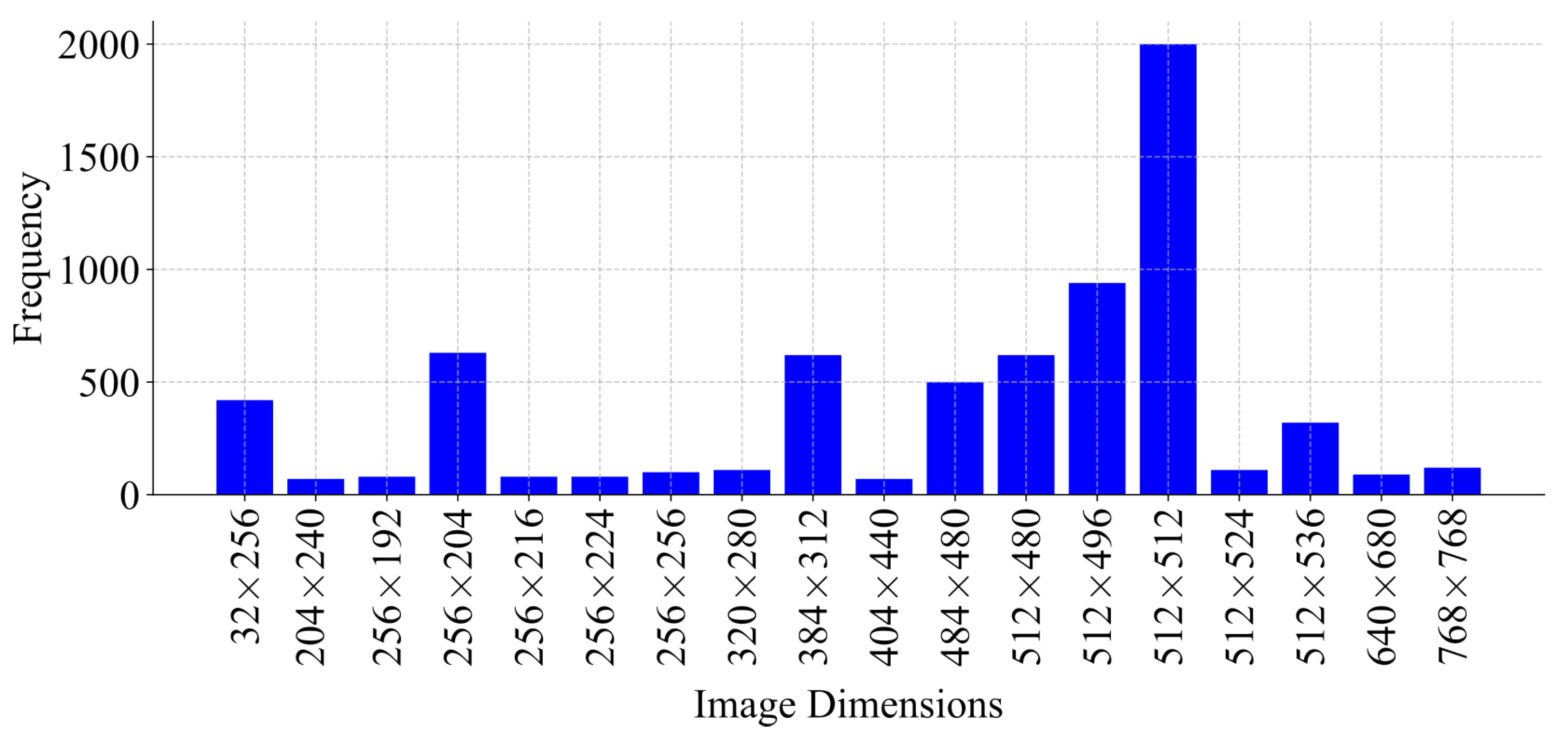
An analysis of the dimensions of these images was conducted, revealing variability not only across different patients but also within the same patients (Figure 4). A resolution of 512 × 512 pixels was the most frequently observed, justifying its selection as the image standard dimension for preprocessing. Therefore, all images were resized to 512 × 512 pixels due to the predominant frequency in the data set. Images smaller than this resolution were padded, while larger images maintained uniformity.

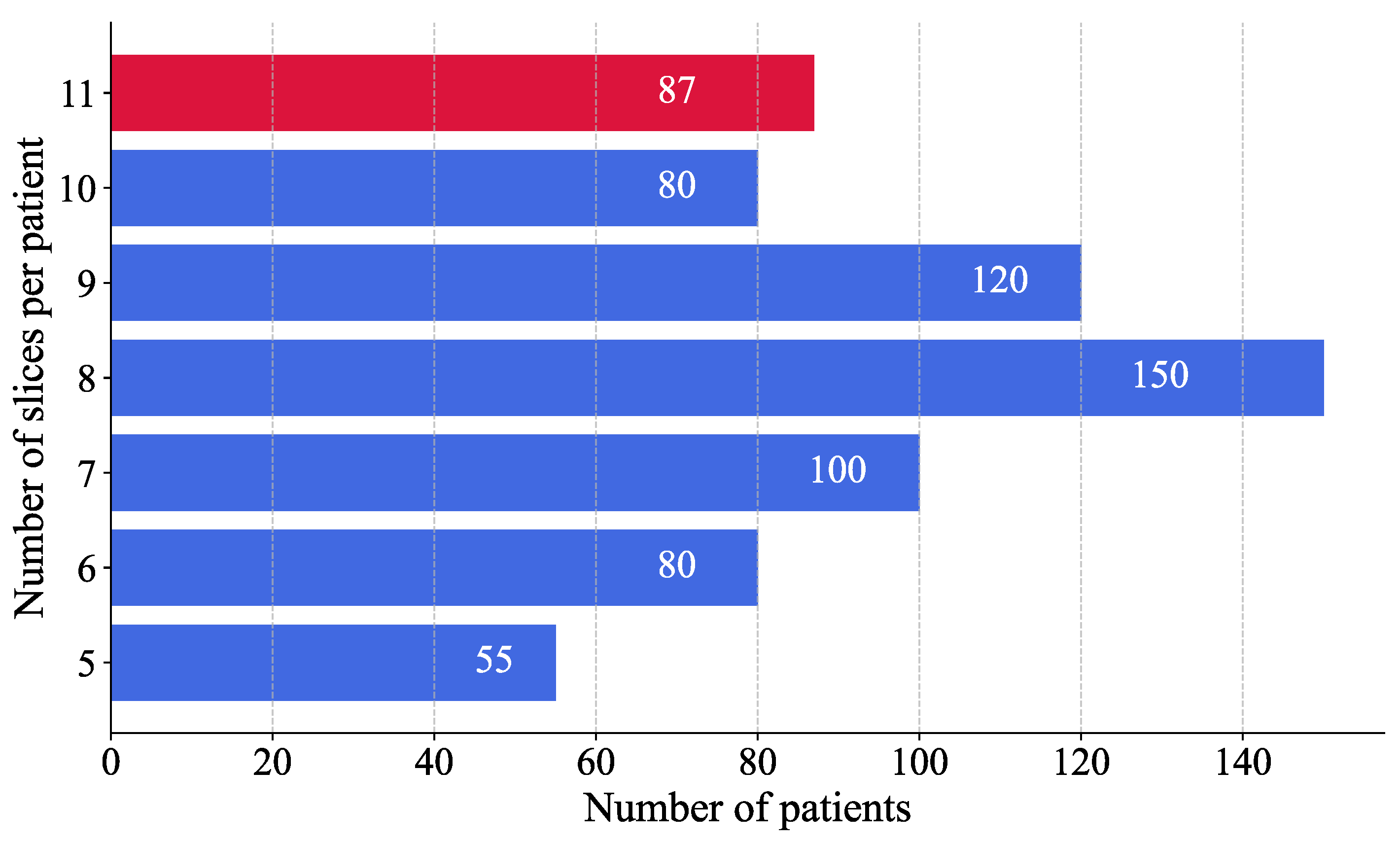
A histogram analysis was performed to assess the distribution of MRI images per patient (Figure 5). The results showed that most patients had eight images. To ensure consistency across patient data and to avoid excluding individuals with fewer available MRI slices, the number of images per patient was standardised to eight, thereby maximising patient inclusion and minimising information loss. This selection, based on the modal value, facilitated the reconstruction of a volumetric representation of the brain from the most informative slices, approximated to a three-dimensional structure.

For patients with more than eight images, a binary mask was applied to each image to convert the values 0 to 255 into a binary scale, where pixels with a value greater than 1 were set to 1 and those with a value greater than 0 remained unchanged. This process identified images with the most significant informational content by measuring the area of non-zero pixels. Only the eight images with the highest information content were retained to ensure uniformity across the data set. In contrast, patients with less than eight images, the image containing the maximum diagnostic information was duplicated until eight images were reached, thereby preserving uniformity across the data set.

The impact of CNN depth on the performance of the GBM classification model was systematically analysed. A range of CNN configurations were evaluated, varying both the number of layers and the number of neurons per layer. Each value in the configuration sequence represents the number of neurons in the corresponding layer, illustrating the progressive increase in model complexity. The tested configurations ranged from simpler architectures with fewer layers and neurons {8, 16, 32} to more intricate structures, incorporating additional layers and higher neuron counts {8, 16, 32, 64, 128, 256}.

In order to select the optimal architecture, an incremental experiment was conducted, by progressively increasing the number of layers manner and evaluating their impact on the AUC-ROC metric. For each configuration, a different model was constructed using the Adam optimiser and a binary cross-entropy loss function for compilation. The models were evaluated through 5-fold cross-validation ($k=5$), wherein the data set was divided into five equal parts, with each subset serving once as the validation set while the remaining as the training sets [39]. This approach ensured that each sample was used for both training and validation, improving robustness and generalisation. The training was performed with a learning rate of $1\times {10}^{-3}$, a batch size of 64, and a total of 200 training epochs. The model converged within 120 epochs, indicating stable performance across different depths.

A clear correlation between model performance and network architecture complexity was observed during the evaluation of CNN on the validation set. This complexity was mainly characterised by the number of convolutional layers. As shown in Figure 6, the first experiment with a single-layer configuration {8} exhibited a baseline validation accuracy of approximately 32%. With the increasing depth of the architecture, the accuracy improved gradually to about 45% in architectures comprising more sophisticated configurations, such as {8, 32} and {8, 16, 32, 64}, which correspond to convolutional networks of three and four layers. The enhancement of accuracy was observed with the five-layer configuration {8, 16, 32, 64, 128}, which reached and stabilised at around 61% ± 0.3.

Models comprising fewer than five layers were found to lack the capacity to extract relevant features from MRI images, resulting in lower performance. Although deeper architectures, such as six-layer models, exhibited slightly higher performance, they introduced a greater standard deviation (0.038), indicating diminishing returns and potential overfitting.

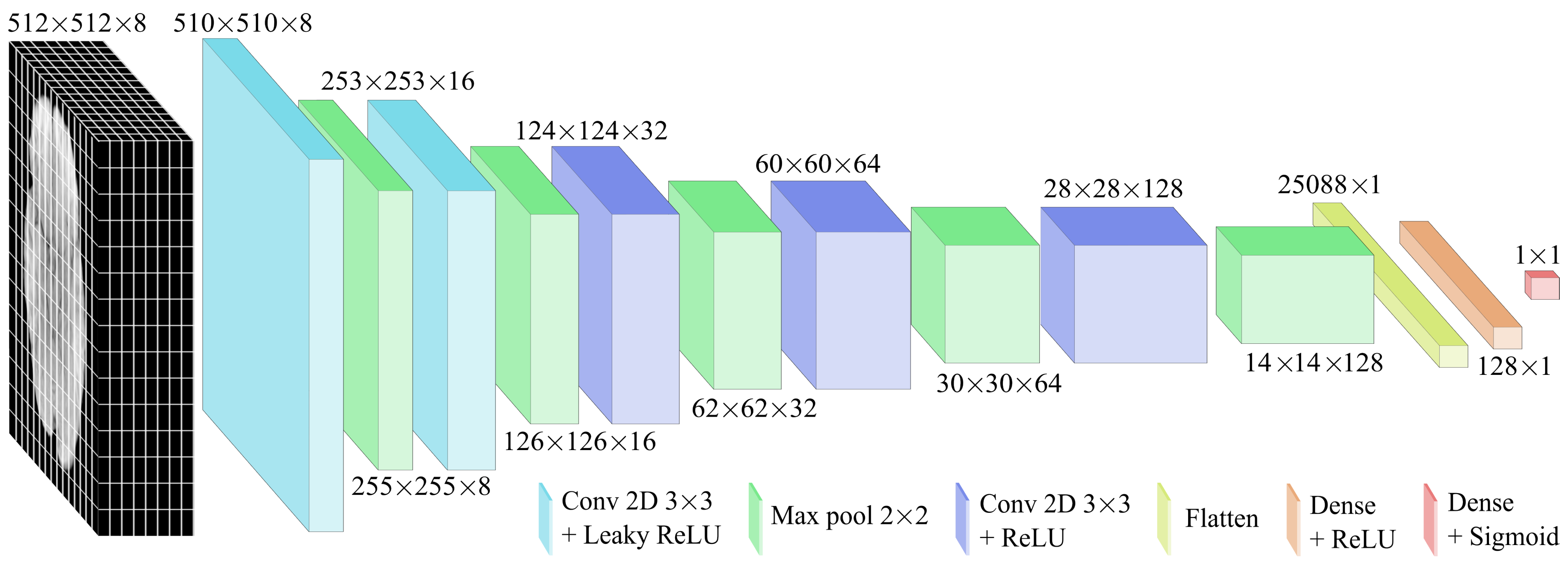
Based on these observations, the five-layer configuration was selected for final optimisation and evaluation. As shown in Figure 7, this structure enabled the modelling of complex hierarchical patterns while maintaining stable training. Accordingly, two activation functions were applied based on their advantages. The Leaky ReLU function was used in the initial layers to mitigate the dead-neuron problem and improve the gradient flow for negative inputs, while ReLU was employed in deeper layers due to its computational efficiency and effectiveness in image processing. The specifications of the CNN model are detailed in

Table 3. The CNN model architecture.

Layers	Filter Size	No. Filters	Activation	Output	TP
InputLayer	N/A	N/A	N/A	(64, 512, 512, 8)	0
Conv2D	$3\times 3$	8	Leaky ReLU	(64, 510, 510, 8)	224
MP	$2\times 2$	N/A	N/A	(64, 255, 255, 8)	0
Conv2D	$3\times 3$	16	Leaky ReLU	(64, 253, 253, 16)	1168
MP	$2\times 2$	N/A	N/A	(64, 126, 126, 16)	0
Conv2D	$3\times 3$	32	ReLU	(64, 124, 124, 32)	4640
MP	$2\times 2$	N/A	N/A	(64, 62, 62, 32)	0
Conv2D	$3\times 3$	64	ReLU	(64, 60, 60, 64)	18,496
MP	$2\times 2$	N/A	N/A	(32, 30, 30, 64)	0
Conv2D	$3\times 3$	128	ReLU	(64, 28, 28, 128)	73,856
MP	$2\times 2$	N/A	N/A	(64, 14, 14, 128)	0
Flatten	N/A	N/A	N/A	(64, 25,088)	0
Dense	N/A	128	ReLU	(64, 128)	N/A
Dense	N/A	1	Sigmoid	(64, 1)	N/A
Loss: Binary Cross-Entropy

Note: MP stands for MaxPooling2D, and TP stands for trainable params.

.

The Adam optimiser was selected for its adaptive learning rate properties, enabling efficient training and noise management. In order to determine the optimal configuration, a hyperparameter tuning process was performed by assessing several combinations of learning rates and batch sizes.

This exploration aimed to balance convergence behaviour and performance across evaluation metrics. As shown in

Table 4. Results of hyperparameter tuning. Bold text and green shading indicate the best-performing configuration across all evaluation metrics.

No	Hyperparameters		Evaluation Metrics
	LR	Batch Size	Accuracy	AUC-ROC	F1-Score	Precision
1	1 × 10−3	32	45.2 ± 0.21	50.0 ± 0.39	62.3 ± 0.32	45.2 ± 0.28
2	1 × 10−4	32	58.9 ± 0.15	60.1 ± 0.12	61.2 ± 0.36	53.5 ± 0.28
3	1 × 10−5	32	58.1 ± 0.11	57.8 ± 0.39	54.5 ± 0.35	53.7 ± 0.16
4	1 × 10−3	64	66.7 ± 0.16	67.7 ± 0.19	68.2 ± 0.26	60.0 ± 0.23
5	1 × 10−4	64	55.5 ± 0.28	57.9 ± 0.14	62.8 ± 0.19	50.5 ± 0.21
6	1 × 10−5	64	58.9 ± 0.34	60.5 ± 0.16	63.1 ± 0.25	53.2 ± 0.28
7	1 × 10−3	128	59.8 ± 0.28	58.5 ± 0.15	60.5 ± 0.12	57.1 ± 0.38
8	1 × 10−4	128	56.4 ± 0.34	56.7 ± 0.19	55.6 ± 0.13	51.6 ± 0.31
9	1 × 10−5	128	56.4 ± 0.14	56.1 ± 0.25	52.3 ± 0.11	51.8 ± 0.37
10	5 × 10−3	32	60.6 ± 0.30	61.1 ± 0.19	60.3 ± 0.26	55.5 ± 0.26
11	1 × 10−4	32	59.8 ± 0.30	60.5 ± 0.31	60.5 ± 0.32	54.5 ± 0.29
12	5 × 10−5	32	55.5 ± 0.38	56.2 ± 0.13	56.6 ± 0.16	50.7 ± 0.11
13	5 × 10−3	64	58.1 ± 0.22	58.9 ± 0.18	59.5 ± 0.35	52.9 ± 0.21
14	1 × 10−2	64	60.6 ± 0.26	61.1 ± 0.14	60.3 ± 0.34	55.5 ± 0.12
15	1 × 10−5	64	57.2 ± 0.33	58.1 ± 0.16	59.1 ± 0.10	52.1 ± 0.34
16	5 × 10−3	128	54.7 ± 0.32	55.0 ± 0.33	53.9 ± 0.12	50.0 ± 0.21
17	5 × 10−4	128	55.5 ± 0.36	56.2 ± 0.29	56.6 ± 0.20	50.7 ± 0.12

, a learning rate of $1\times {10}^{-3}$ was selected after testing values between $1\times {10}^{-2}$ and $1\times {10}^{-4}$. Higher rates led to oscillations, while lower rates slowed convergence. Furthermore, a batch size of 64 was determined as optimal among the tested values (32, 64, and 128), providing the best balance between speed and convergence stability. The model architecture consisted of 98.38 ×${10}^3$ trainable parameters, requiring approximately 384.3 kilobytes of memory, with 32-bit precision (4 bytes per parameter). This configuration enabled computational efficiency, facilitating rapid iterations during the development of the training pipeline.

Predictions were generated for the 87 patients in the hidden test set and submitted to the Kaggle platform, for model evaluation using the AUC-ROC metric. The model achieved a score of 0.63, surpassing all 1000 participating researchers and setting a new state of the art (

Table 5. BraTS 2021 challenge results.

#	Team	Score
1	Tunisia	0.62
2	Minh Phan	0.61
3	Cedric Soares	0.61
4	Leaky Folds	0.61
5	Random	0.61
6	Proposed Method	0.63

). The results are available in the “leaderboard” section of the Brain Tumor Radiogenomic Classification Challenge, conducted as part of the BraTS 2021 challenge, sponsored by the Radiological Society of North America and the Medical Image Computing and Computer Assisted Intervention Society. The reported scores are available in [40].

3.2. Inference of the CNN Model on the EGD Data Set for Glioma Detection

The model was evaluated in the EGD data set, which contains clinical history data such as age and sex, to determine correlations with the model prediction. Figure 8 summarises the model predictions in the Erasmus database, composed mainly of patients with glioma. Consequently, the bar graph represents only the TP and FP counts, while TN and FN values were absent due to the database inherent design.

The results showed that the model was generalizable across both age and sex groups, achieving an F1-score of 0.88 (

Table 6. Model performance metrics.

Metric	Value
F1-Score	0.88
Precision	0.78
False Negative Rate	0.21

). However, in older patients, model predictions were more accurate, with an average accuracy of 57.29 years (±14.68) compared to 54.55 years (±14.22) of incorrect predictions (

Table 7. Statistical summary of predictions by age and sex.

Prediction	Age (M ± SD)	Range	Preds	M	F
Incorrect	54.55 ± 14.22	21–82	155	94	61
Correct	57.29 ± 14.68	19–86	570	362	208

). Furthermore, a sex-based comparison revealed a slightly higher correct prediction rate for men (79.39%) than women (77.70%) (

Table 8. Distribution of incorrect and correct predictions by sex in the Erasmus Glioma Database (EGD) data set.

Sex	Incorrect Predictions	Correct Predictions
Female	61	208
Male	94	362

).

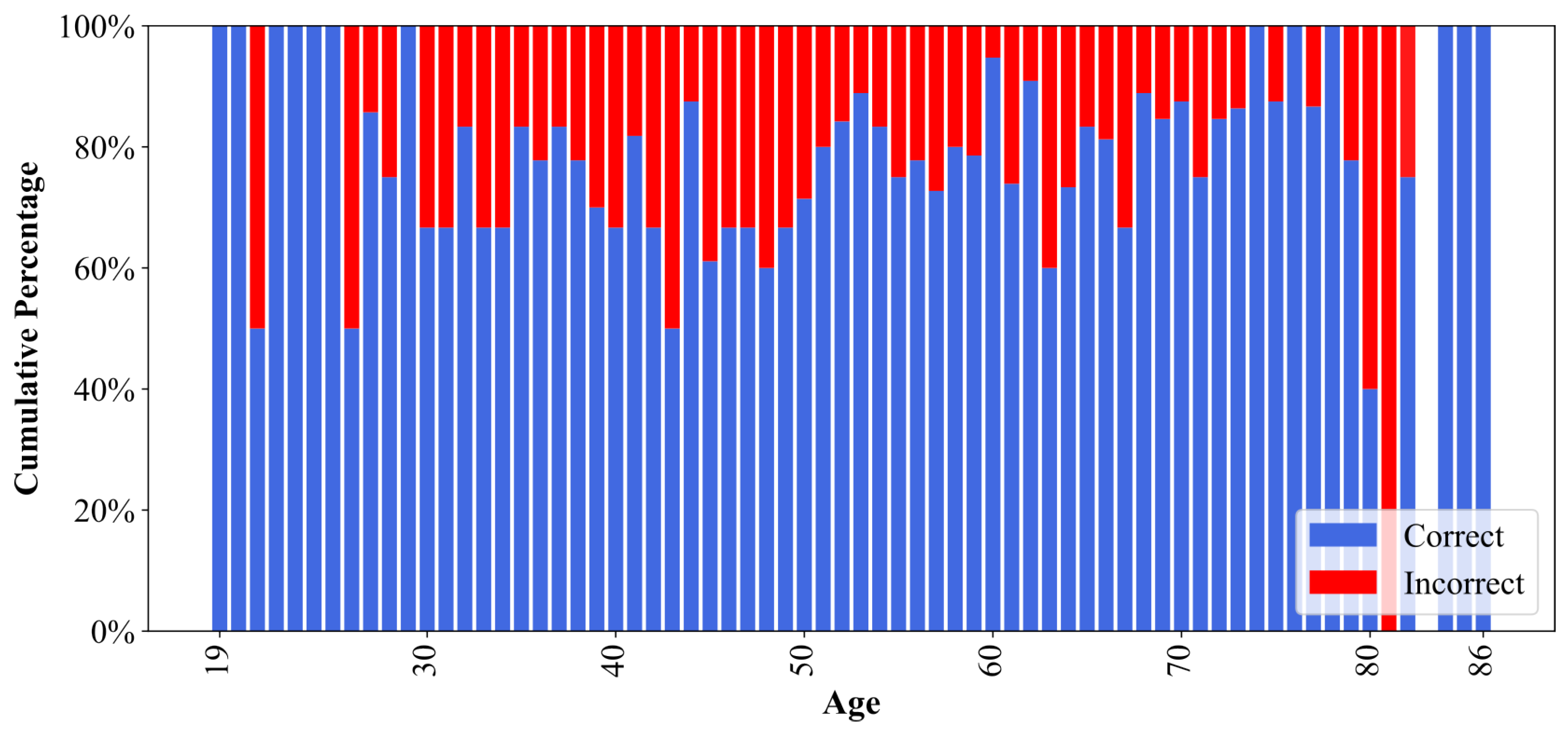
Although both groups exhibited comparable performance, the slight variations based on demographic factors suggested the possibility of subtle influences. As illustrated in Figure 9, the model demonstrated suboptimal predictive accuracy for patients aged 80–81 years, with correct prediction rates falling below 50%. This led to an investigation into the potential bias in model predictions.

Statistical Analysis for Assessment of Demographic Bias

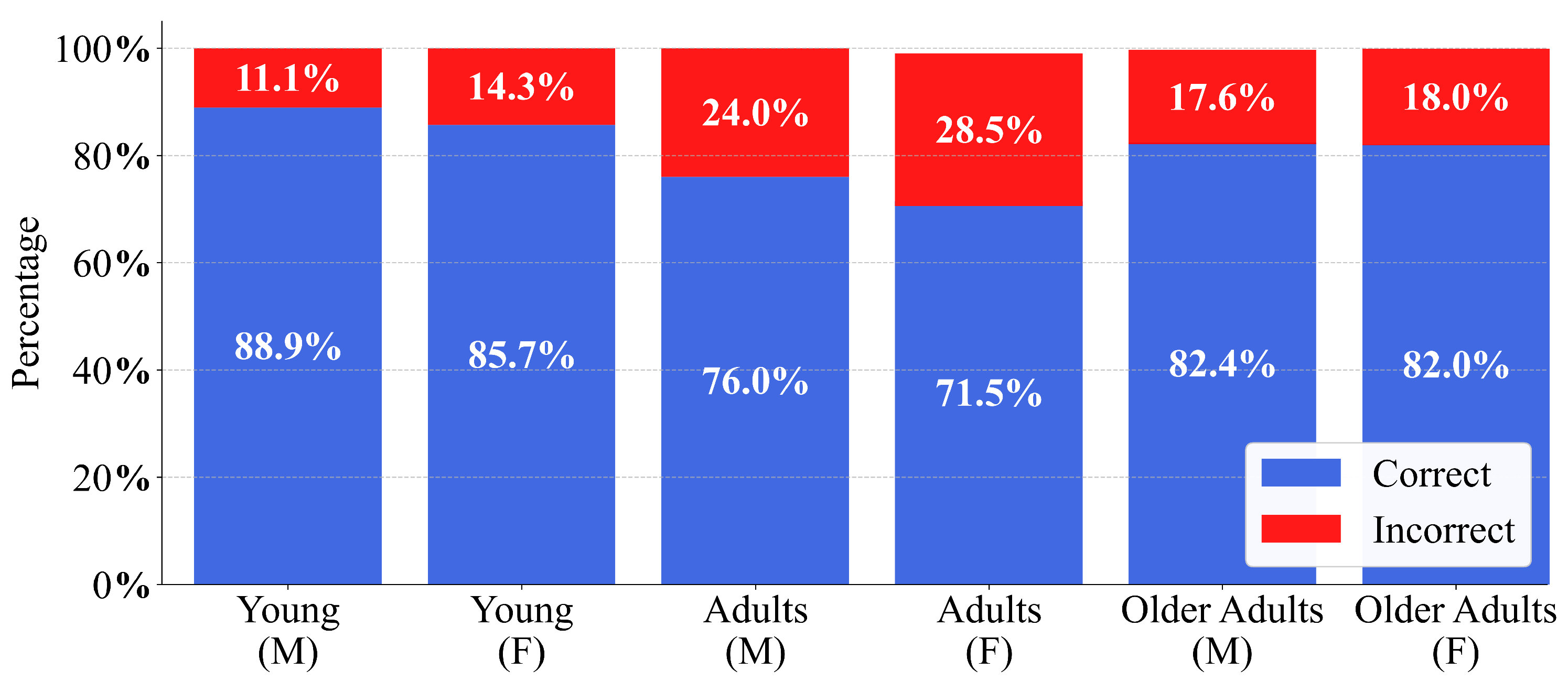
To analyse any significant variation in model performance, the patient cohort was stratified into three age groups: young (19–26 years), adults (27–59 years), and older adults (60–100 years) for both sexes, as proposed in [41]. As illustrated in Figure 10, this age segmentation revealed a trend among age groups of both men and women, with the highest percentage of errors observed in adults, followed by older adults and then young patients, and slightly more pronounced in women. This led to the application of statistical tests to corroborate whether demographic factors, such as age and sex, exerted a significant influence on model performance and may have contributed to potential discrepancies in the predictions.

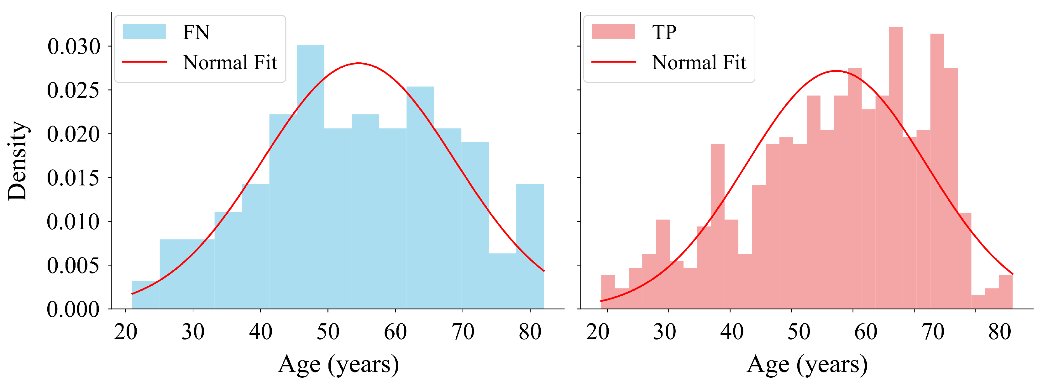
To assess the normal age distribution in the FN and TP groups (Figure 8), the Shapiro–Wilk test was applied under the following hypotheses:

H₀. 

The data follows a normal distribution.

H₁. 

The data do not follows a normal distribution.

As outlined in

Table 9. Shapiro–Wilk test, confidence intervals, and power analysis for age distributions. W represents the Shapiro-Wilk statistic and n denotes the sample size.

Group	Power	n	Mean Age ($\overline{\mathit{x}}$, $\mathit{\sigma }$)	95% CI	W	p-Value
FN	0.924	155	54.55 (14.22)	[52.32, 56.79]	0.984	0.120
TP	0.998	570	57.29 (14.68)	[56.09, 58.50]	0.989	0.003

, the results of the Shapiro–Wilk test showed that the obtained p-value for the FN group followed a normal distribution. Conversely, the TP group exhibited a p-value lower than $\alpha$, indicating a deviation from normality (Figure 11). Regarding the confidence intervals, the slight overlap between the intervals $56.08$ and $56.79$ suggested that the difference between the two groups was not significant.

To evaluate differences in age distributions between prediction outcome groups within each cohort, the Mann–Whitney U test was applied under the following hypotheses:

H₀. 

The distribution of ages differs between groups.

H₁. 

There is an association between sex and prediction correctness.

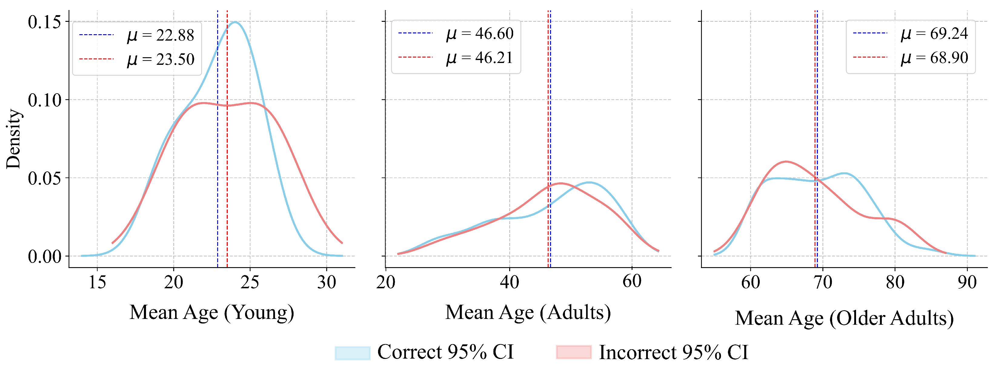
As shown in

Table 10. Results of the Mann–Whitney U test by age cohorts, including power analysis and confidence intervals. $n_1$ denotes the FN predictions, U represents the Mann–Whitney statistic and Z represents the normal statistic. The symbols and × correspond to the correct and incorrect predictions, respectively.

Group	Power	${\mathit{n}}_1$	95% CI		U	Z	p-Value
			✓	×
Young	0.133	4	[20.67, 26.33]	[21.75, 24.00]	38.0	0.567	0.599
Adults	0.757	90	[44.51, 47.91]	[45.52, 47.67]	11,440.5	−0.729	0.466
Older Adults	0.782	61	[67.30, 70.50]	[68.53, 69.95]	8332.0	−0.550	0.583

, the results of the Mann–Whitney U test indicated that none of the three age cohorts showed sufficient statistical evidence to reject $H_0$, suggesting the absence of age-related bias in model predictions. Regarding the confidence intervals, the 95% CIs for the difference in medians reinforce the lack of substantial differences between subgroups (Figure 12). The obtained power values were calculated with the shift for each age cohort extracted from their data distributions. Despite the power values obtained for certain cohorts, the p-values further support the acceptance of the null hypothesis.

To evaluate the association between sex and the correctness of model predictions, the Chi-squared test was applied under the following hypotheses:

H₀. 

There is no association between sex and prediction correctness.

H₁. 

There is an association between sex and prediction correctness.

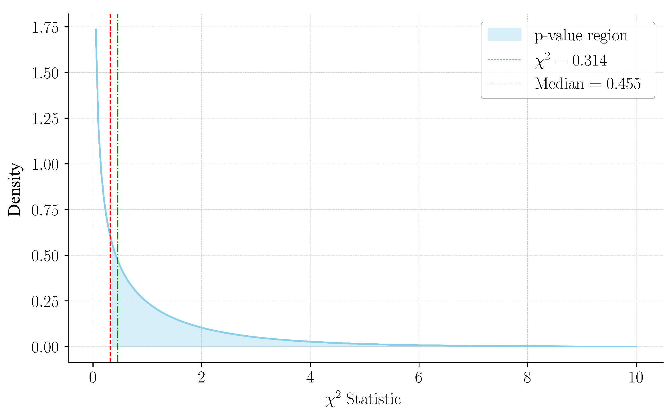
As detailed in

Table 11. Chi-squared test, confidence interval, and power analysis for prediction correctness by sex. ${\chi }^2$ represents the Chi-squared statistic, and n denotes the total sample size.

Test	Power	n	95% CI	${\mathit{\chi }}^2$	p-Value
Chi-Squared	0.99	725	[33.08, 88.85]	0.314	0.575

, the computed Chi-square statistic was 0.314, with a corresponding p-value of 0.575. The p-value was calculated as $P({\chi }^2\ge 0.314)$. Since the statistic lies below the median of the distribution (${\chi }_{0.5,1}^2\approx 0.455$), this aligns with a non-significant result, as visualized in Figure 13. The power analysis indicated a moderate capacity to detect a small effect size, thereby reinforcing the reliability of the results. These findings suggested that the statistical analysis did not provide strong evidence to confirm differences in accuracy based on sex, thereby supporting the generalisability of the model.

4. Discussion

The proposed CNN model achieved an AUC-ROC of 0.63 on the RSNA-MICCAI data set, surpassing all previous submissions to the BraTS 2021 challenge [21]. This result positions the model as the current benchmark within this evaluation framework. The model was trained on skull-stripped T1-weighted MRIs and subsequently applied to the EGD, which includes full-head scans with different anatomical representations. Despite these morphological and acquisition differences, the model achieved an F1-score of 0.88, a precision of 0.78, and a false negative rate of 0.21 on the EGD data set [23].

In prior work on MRI-based glioma classification, researchers generally trained and tested CNN models on the same data set without external validation or bias analysis [42,43,44,45]. Notably, Chang et al. [42] trained a CNN to predict genetic mutations (e.g., IDH1) in gliomas from MR images and reported accuracy using only internal train/test splits. Zhuge et al. [43] developed 3D CNN pipelines to grade gliomas using BraTS-2018 and TCGA-LGG via five-fold cross-validation. Gutta et al. [44] and McAvoy et al. [45] also used single-institutional data sets or limited validation. None of these studies performed external evaluation or assessed demographic bias. In contrast, our study incorporates cross-data set validation and statistical bias testing, addressing both generalisation and fairness.

To assess the fairness of model predictions, a statistical evaluation was conducted. The Mann–Whitney U test did not identify significant differences in age distributions between correct and incorrect predictions within age cohorts, with p-values of 0.599, 0.466, and 0.583 for young, adult, and older adults, respectively. Similarly, the Chi-squared test showed no significant association between sex and prediction correctness (${\chi }^2=0.314$, $p=0.575$). Confidence intervals overlapped, and power analyses confirmed test sensitivity to moderate effects. These results support the absence of demographic bias. Unlike previous works reporting performance variability due to imbalance or hidden covariates [46], our model showed consistency across demographic subgroups. Although CNNs can internalise latent patterns that lead to disparities [46], the methodology applied here reinforces the robustness of our findings. This aligns with best practices in fairness-aware AI and contrasts with studies where data set imbalance introduced bias [47].

The preprocessing strategy contributed to the performance of the model and generalisation. Non-informative slices (27.7%) were excluded, and all images were resampled to a common resolution. Input was restricted to T1-weighted MRIs, and intensity normalisation was applied. Prior work has shown that such standardisation improves classification accuracy [48]. In contrast, other studies have used raw or mixed-contrast inputs without consistent filtering or resolution adjustment, increasing heterogeneity in training data. The architecture was also optimised through systematic analysis of depth and capacity, rather than adopting generic CNNs. Studies using fixed designs, such as VGG-like architectures, report lower performance under similar conditions [49].

Unlike previous CNN-based methods that incorporate multiple MRI modalities like T2w, FLAIR, or diffusion sequences, this study introduces a technique that uses only T1w MRI images for input. T1w images deliver excellent contrast between tumours and adjacent brain tissue and possess the necessary anatomical details for detecting and assessing gliomas. Research has demonstrated that relying solely on T1w images can achieve competitive classification results while streamlining the acquisition process [50,51]. Furthermore, merging multiple modalities demands precise registration and alignment across sequences, which increases computational demands and introduces potential errors [52]. By focusing on a single modality, this approach decreases the model’s input dimensionality and removes cross-modality preprocessing, thus enhancing inference speed.

The model demonstrated generalisation and demographic fairness across data sets. To support its use in clinical settings, future work should include validation in prospective medical environments. This step will confirm its applicability in real-world diagnostic workflows and complement the current evidence.

5. Conclusions

This study reports advances in the diagnosis of GBM using CNN, achieving an AUC-ROC score of 0.63 in the RSNA-MICCAI data set, which exceeds previous results and thereby establishes a new state-of-the-art within this specific evaluation framework. Furthermore, the model demonstrates detection capabilities by generalising to lower-grade gliomas. A comprehensive preprocessing strategy was applied to the MRI images, which played a key role by eliminating irrelevant data and ensuring consistency in the input images to the model. Notably, although the RSNA-MICCAI data set consists of skull-stripped images, while the EGD data set preserves full cranial anatomy, the model achieved an F1-score of 0.88, demonstrating generalisation across data sets with different anatomical representations. In addition, a statistical analysis of demographic biases, such as age and sex, does not reveal a significant influence on predictions. Although small performance differences were observed in favour of older male patients, these variations were not statistically significant.