A Hybrid Adaptive Particle Swarm Optimization Algorithm for Enhanced Performance

Abstract

The traditional particle swarm optimization (PSO) algorithm often exhibits defects such as of slow convergence and easily falling into a local optimum. To overcome these problems, this paper proposes an enhanced variant featuring adaptive selection. Initially, a composite chaotic mapping model integrating Logistic and Sine mappings is employed to initialize the population for diversity and exploration capability. Subsequently, the global and local search capabilities of the algorithm are balanced through the introduction of adaptive inertia weights. The population is then divided into three subpopulations—elite, ordinary, and inferior particles—based on their fitness values, with each group employing a distinct position update strategy. Finally, a particle mutation strategy is incorporated to avoid convergence to local optima. Experimental results demonstrate that our algorithm outperforms existing algorithms on the standard benchmark functions. In practical engineering applications, our algorithm also has demonstrated better performance than other meta heuristic algorithms.

1. Introduction

As technology advances and societal needs evolve, optimization techniques have become essential across various industries. Traditional optimization methods frequently encounter difficulties when addressing complex, multidimensional challenges, which complicates the pursuit of optimal solutions. This has spurred increased interest in the development of more efficient and intelligent optimization algorithms. One notable example is particle swarm optimization (PSO) [1], which is distinguished by its capacity to address both mixed-space and continuous optimization problems, thus serving as a valuable tool. PSO has been effectively applied in numerous domains, including parameter optimization [2], neural network training [3], clustering analysis [4], combinatorial optimization [5], pattern recognition [6], and image processing [7]. Furthermore, the intelligent optimization capabilities of PSO present significant potential for advancement in artificial intelligence [8] and machine learning [9]. By conducting comprehensive research on the PSO algorithm, we can gain deeper insights into its underlying mechanisms and performance, thereby facilitating its enhancement and wider application.

Numerous researchers have made great efforts to enhance PSO algorithms in terms of running performance, convergence, and parameter settings. To address high-dimensional complex problems, Shi et al. introduced a novel method for adjusting the inertia weight factor, which they modified to decrease linearly from 0.9 to 0.4 [10]. Subsequently, they adjusted the inertia weights to random values between 0.5 and 1 and designed a new algorithm, PSO-RIW, which demonstrated improved robustness in experimental tests [11]. Ratnaweera et al. proposed a variable acceleration factor mechanism that proved more effective than time-varying inertia weights for optimizing single-peak functions in simulations [12]. Arumugam et al. introduced the GLBEST-PSO algorithm, which modifies inertia weights by averaging the global and individual optima during iterations [13]. Chegini et al. developed the PSOSCALF algorithm by integrating the hybrid PSO algorithm, the positive cosine algorithm, and Levy’s flight method, thereby enhancing the exploration capabilities of PSO and influencing local optimal positions with a degree of temptation [14]. A recent study [15] introduced a self-learning strategy alongside a nonlinear weight factor strategy aimed at enhancing the local search capabilities of the algorithm. This was achieved by employing Levy’s flights to perturb the positions of the population, thereby assisting in escaping local optima. The authors of [16] presented a normal cloud model designed to adjust both the range of the wolf population’s positions and the optimal individual, as well as the dispersion of the wolf population. This approach effectively improved the algorithm’s local exploitation ability and convergence accuracy. Furthermore, several novel metaheuristic algorithms have been developed, including the dung beetle optimization algorithm [17], the vulture search algorithm [18], the sand cat swarm optimization algorithm [19], and the adaptive hybrid variational differential evolution (a-HMDE) [20]. Dixit et al. [21] proposed a new differential evolutionary algorithm based on particle swarm optimization, which utilizes differential evolution variants in the initial stages to broaden the search space, identify more promising solutions, and mitigate the risk of premature convergence. Seyyedabbasi et al. [22] introduced the comprehensive learning particle swarm optimizer (CLPSO) for addressing complex multimodal problems. This method leverages the historical optimal experiences of other particles to enhance population diversity and global search capabilities. Concurrently, some researchers have integrated concepts from various optimization algorithms to improve convergence speed and search accuracy. These advancements have facilitated the widespread application of PSO in power network optimization [23], mechanical design innovation [24], and logistics and distribution scheduling [25].

Although a lot of research has been conducted on the PSO algorithm, the main problems of the algorithm have not been fully solved. First, the algorithm itself has the problem of premature convergence. For example, when the algorithm uses complex multi-peak functions, it is easy to fall into local optimization. Meanwhile, the algorithm is highly sensitive to parameter settings such as inertia weights and acceleration coefficients, but there is no generalized parameter setting mechanism. Second, it often faces an imbalance between global and local search. Too much focus on the global search capability leads to inefficiency and slow convergence, while too much emphasis on the local search capability increases the risk of falling into a local optimum. Third, when facing a high-dimensional optimization problem, the search space exponentially expands, leading to a significant increase in computational complexity, and the algorithm is more likely to converge to a local optimum. In addition, the interaction mechanism between particles is complex, making it difficult to effectively guide the search direction. In practice, engineering optimization problems often contain both equal and unequal constraints. In such scenarios, methods need to be developed that can handle these constraints while maintaining the performance of the algorithm. Therefore, improvements to the algorithms still require significant work.

This paper proposes an adaptive selection particle swarm optimization algorithm and investigates its applications. Central to the algorithm is the integration of enhancement strategies into the standard particle swarm approach, which allows the particles to perform a more nuanced search within the solution space, thereby enhancing population diversity. The enhancement strategies examined in this paper include the following:

• Initializing the particle swarm using hybrid chaotic mapping to achieve a more uniform distribution of the population within the solution space, thereby enhancing population diversity.
• Focusing on dynamically adjusting the inertia weights through adaptive weights, allowing particles to conduct precise searches at each stage.
• Dividing the population into three subsets and updating the velocity and position of the particles by applying cross-learning and social learning mechanisms to the elite particles, which aims to improve the exploration performance of the particles.
• Employing the evolutionary strategies DE/best/1 and DE/rand/1 on ordinary particles to enhance their utilization, while also introducing a mutation mechanism to prevent the improved algorithm from converging on local optimal solutions during the search process.

A variety of strategies, including composite chaotic mapping for population initialization, adaptive inertia weights, an elite particle learning mechanism, and a differential evolution strategy for ordinary particles, are integrated to develop a novel particle swarm optimization algorithm referred to as APSO. This integration seeks to enhance the algorithm’s search efficiency, mitigate convergence to local optima, and bolster its robustness. To assess the effectiveness of the improved APSO algorithm, we conduct tests and comparisons with other algorithms, evaluating the optimal value, standard deviation, and average value for each. Ultimately, the algorithm is applied to real-world engineering problems to derive practical solutions.

2. PSO Algorithm

This section provides a thorough overview of the fundamental concepts and equations underlying the traditional particle swarm optimization algorithm, including a detailed explanation of the parameters utilized in these equations. Furthermore, due to the flowchart that delineates the steps of the algorithm, readers can achieve a clearer understanding of the particle swarm optimization process.

2.1. Principle

The PSO algorithm is a widely recognized method of population-based intelligent optimization. Similar to other algorithms in this category, it typically commences by randomly initializing a set of solutions, referred to as particles. The algorithm then iteratively updates these solutions, guiding the entire population toward enhanced fitness. The ultimate objective is to identify the optimal solution to the problem within a constrained number of iterations.

If the PSO algorithm with N particles is employed to address a problem within a search space of dimension J, the position and velocity components of the i-th particle (where $1\le i\le N$) at the n-th iteration can be expressed as $X_i=(x_{i1},x_{i2},\dots ,x_{ij},\dots ,x_{iJ})$ and $V_i=(v_{i1},v_{i2},\dots ,v_{ij},\dots ,v_{iJ})$, respectively. During each iteration, PSO employs specific formulas to update the velocity and position of each particle in each dimension component:

$$v_{ij}^{t+1}=v_{ij}+c_1{r}_1({pBest}_{ij}^t-x_{ij}^t)+c_2{r}_2(gBes{t}_{gj}^t-x_{ij}^t),$$

(1)

$$x_{ij}^{t+1}=x_{ij}^t+v_{ij}^{t+1}$$

(2)

Equations (1) and (2) present the updated iterative formulas of the original PSO algorithm [1]. In these equations, $c_1$ and $c_2$ represent acceleration factors that are utilized to modify the convergence speed, typically assuming a value of 2. $r_1$ and $r_2$ are random numbers distributed on [0, 1]; $x_{ij}^t$ denotes the position component of the j-dimensional space of particle i in the t-th iteration; ${pBest}_{ij}^t$ denotes the optimal position of an individual; ${gBest}_{gj}^t$ denotes the optimal position of a group; after the completion of each iteration, the $pBest$ position of each particle must be updated according to the following rules:

$$p_{ij}^{t+1}=\left\{\begin{array}{c}\hfill x_{ij}^{t+1},f\left(X_{ij}^{t+1}\right)<f\left(p_{ij}^t\right),\\ \hfill p_{ij}^t,f\left(X_{ij}^{t+1}\right)\ge f\left(p_{ij}^t\right).\end{array}\right.$$

(3)

where $f(•)$ represents the objective function used to determine the corresponding positional adaptation value. In many cases, it is necessary to confine particle velocities within a specific interval, denoted as $[-v_{max},v_{max}]$, to align with the practical requirements when employing the algorithm. However, researchers have observed that the initial version of the algorithm exhibited slow convergence rates when addressing certain problems, primarily due to its overly global search behavior. This limitation resulted in diminished algorithm performance. To address this issue, Shi and Eberhart [11] introduced an enhanced PSO algorithm incorporating inertia weights, which involves the addition of inertia weights to Equation (4):

$$v_{ij}^{t+1}=\omega v_{ij}+c_1{r}_1\left(pBes{t}_{ij}^t-x_{ij}^t\right)+c_2{r}_2\left(gBes{t}_{gj}^t-x_{ij}^t\right)$$

(4)

The formula consists of three components: the first is termed the ’inertia component, which reflects the influence of the particle’s inertia weights on its current velocity state, thereby preventing excessive oscillation during the search process. The inertia weights, denoted as $\omega$, decrease linearly from 0.9 to 0.4 over the course of the iterations. This algorithm has been demonstrated to outperform alternative versions in numerous experiments and applications, and is therefore referred to as the standard PSO algorithm [26]. Unless otherwise specified, all references to the PSO algorithm in the subsequent sections pertain to the standard PSO algorithm. The second component is the “individual cognition” of the particle, which represents its learning regarding its own position. The third component is the “social cognition” of the particles, which reflects their learning of the optimal position within the group.

The superposition of “individual cognition” and “social cognition” allows particles to engage in what is termed “partial local search”, while the “inertial part” facilitates “partial global search”. Furthermore, this combination enables particles to execute a “biased global search”. These concepts are derived from the long-term search process, illustrating the overall trend of search behavior rather than defining absolute “global” or “local” search behaviors. Consequently, the flight speed in particle swarm optimization primarily consists of these three components, guiding the particles within the population to converge to a single point gradually.

2.2. Algorithm Implementation

Step 1: Based on the characteristics of the optimization problem, the algorithm randomly initializes several parameters, including the particle swarm size N, the search dimension J, the upper and lower bounds of the search, the maximum number of iterations $t_{max}$, the maximum velocity $v_{max}$, the minimum velocity $v_{min}$, the inertia weight $\omega$, and the learning factors ($c_1$ and $c_2$).

Step 2: The boundaries are assessed based on the initialized positions and velocities of individual particles, followed by the calculation of fitness values. The adaptation values are then sorted, and the velocity and position of the particles are updated in accordance with Equations (3) and (4).

Step 3: Based on the updated velocity and position, the optimal position and optimal fitness of both individual and group particles are revised. A determination is made to ascertain whether the specified condition is met; if so, the process advances to Step 4; if not, it returns to Step 3.

Step 4: Output the optimal solution of the problem.

3. Improved PSO Algorithm

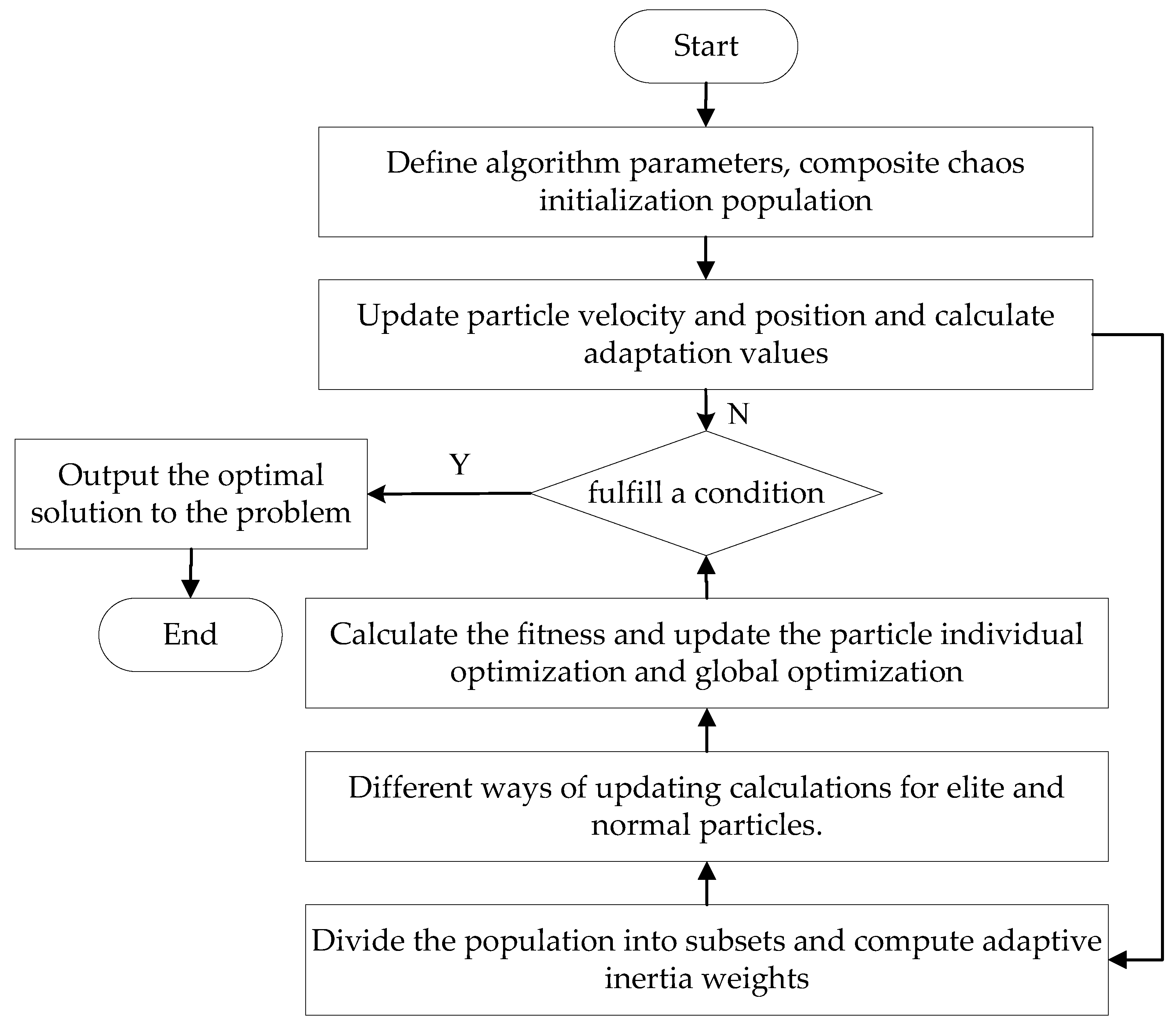
Building upon the standard PSO algorithm, this section introduces four enhancement strategies: composite chaotic mapping for population initialization, adaptive inertia weights, an elite particle learning mechanism, and an ordinary particle mutation strategy. Each of them enhances specific aspects of the standard algorithm, including population initialization, inertia weights, particle velocity and position updates, and cross-mutation. We provide a detailed description of the algorithmic formulas, parameters, and the significance of each improved strategy. Furthermore, a flowchart illustrating the improved adaptive PSO algorithm, referred to as APSO, along with the steps for its implementation, is also presented.

3.1. Complex Chaotic Mapping Initialization Population

In the traditional framework of particle swarm optimization algorithms, the initialization of particle populations typically relies on random methods. However, this random initialization can sometimes result in a less uniform distribution of the population within the solution space, increasing the risk of the algorithm converging to a local optimum. This, in turn, negatively impacts both the search efficiency and solution accuracy of the algorithm. To address this issue, the diversity of the population can be enhanced through chaotic mapping. The fundamental principle involves employing specific mapping techniques of chaotic sequences to translate the optimization variables into chaotic variable space, thereby leveraging the characteristics of chaos to significantly enhance population diversity. Several common chaotic mapping expressions are shown in

Table 1. Common chaotic mappings.

Mapping Type	Formula	Range
Logistic	$x_{k+1}=\gamma x_k\left(1-x_k\right),\gamma \in (0,4)$	$[0,1]$
Cubic	$x_{k+1}=\rho x_k(1+x_k^2)$	$[0,1]$
Chebyshev	$x_{k+1}=cos\left(\alpha {\displaystyle \frac{1}{cos\left(x^k\right)}}\right),\alpha ={\displaystyle \frac{1}{2}}$	$[-1,1]$
Tent	$x_{k+1}=\left\{\begin{array}{cc}{\displaystyle \frac{x^k}{\alpha }},\hfill & x^k<\alpha \hfill \\ {\displaystyle \frac{1-x^k}{1-\alpha }},\hfill & x^k\ge \alpha \hfill \end{array}\right.$	$[0,1]$
Sine	$x_{k+1}=\alpha sin\left(\pi x\right),\alpha \in [0,1]$	$[0,1]$
Sinusoidal	$x_{k+1}=\alpha x_k^{2}sin\left(\pi x\right),\alpha \in [0,4]$	$[0,1]$

.

Different chaotic mappings exhibit distinct properties and exert varying effects on optimization algorithms. Logistic mappings enhance space traversal [27]; however, they may lead to aggregation or spatial white space. In contrast, Sine mappings possess a simpler structure and higher efficiency, which can enhance search accuracy and optimization performance. Tent mappings contribute to a more uniform distribution of particles, although later iterations may transition into a periodic sequence. Cubic and Chebyshev mappings are highly sensitive to initial values, resulting in uneven distribution across the mapping region. Given the numerous limitations associated with traditional chaotic mapping methods, researchers are increasingly favoring optimized chaotic mapping techniques for initializing population-based intelligence optimization algorithms. Among the various optimization schemes, Logistic mapping and Sine mapping are two extensively studied chaotic mapping methods. The composite chaotic mapping that integrates Sine mapping and Logistic mapping offers significant advantages in terms of spatial traversal, population diversity, and distribution uniformity, while also maintaining a simple structure and high computational efficiency [28]. Consequently, we employ a composite chaotic mapping method that combines Sine mapping and Logistic mapping to initialize the population, thereby effectively enhancing the search efficiency and solution accuracy. The specific definition formula and initial value expression for the composite chaotic mapping are presented below:

$$y_i^d={\left(sin\left(\pi y_{i-1}^d\right)\right)}^{aln\left(4b{y}_{i-1}^d\left(1-y_{i-1}^d\right)d+c\right)}$$

(5)

$$x_i^d=lb+y_i^d\times \left(ub-lb\right)$$

(6)

where a, b, c are denoted as the control parameters with the range of values $0\le a\le 1$, $0\le b\le 5$, $1.5\le c\le 5$, respectively; $y_i^d$ and $x_i^d$ denote the random number and the initial value of particle i in the d-th dimension space of the initial position, respectively; $lb$ and $ub$ denote the lower bound and upper bound of the range of values; and the range of values of the particle is $\left[lb,ub\right]$.

To assess the feasibility of the population initialized using composite chaotic mapping, we compare it to a population initialized with a pseudo-random sequence. Figure 1 illustrates the distribution of the composite chaotic mapping initialized population alongside that of the pseudo-random sequence initialized population.

The distribution map clearly indicates that the method of initializing the population using composite chaos effectively integrates the advantages of Sine mapping and Logistic mapping. This approach significantly enhances the uniform distribution of the spatial probability density of the population and improves its spatial traversability [29]. In contrast, initializing the population with a traditional sequence of random numbers, despite demonstrating a high degree of randomness, results in particle aggregation. This aggregation can negatively affect the initial iterations of the algorithm, leading to premature convergence of the particles and potentially trapping them in local optimal solutions. Consequently, the use of composite chaotic mapping for population initialization markedly enhances the efficiency of the algorithmic optimization search and increases the diversity of the population.

3.2. Adaptive Inertia Weights

Adaptive inertia weighting is a mechanism designed to optimize the fitness value by dynamically adjusting the particle inertia weights. This approach allows the algorithm to flexibly modify its search strategy in various situations, thereby enhancing its effectiveness in locating the optimal solution to a given problem. Specifically, when a particle’s fitness evaluation result is lower than the overall performance of the population, the strategy assigns smaller inertia weights to facilitate a fine local search. Conversely, when a particle’s fitness exceeds the average fitness of the population, larger inertia weights are assigned to improve global search capabilities. The expression for these adaptive weights is presented below:

$${\omega }_i^t=\left\{\begin{array}{c}{m}_1,{ftn}_i\left(t\right)\ge {ftn}_{avg}\left(t\right)\hfill \\ m_1+\left\{m_1-m_2\right\}{\displaystyle \frac{ftn\left(t\right)-{ftn}_{gbt}\left(t\right)}{{ftn}_{avg}\left(t\right)-{ftn}_{gbt}\left(t\right)}},{ftn}_i\left(t\right)<{ftn}_{avg}\left(t\right)\hfill \end{array}\right.$$

(7)

where ${\omega }_i^t$ denotes the adaptive inertia weight of particle i at the t-th iteration; $m_1$ and $m_2$ denote the maximum and minimum values of the inertia weights, respectively; ${ftn}_i\left(t\right)$, ${ftn}_{gbt}\left(t\right)$, and ${ftn}_{avg}\left(t\right)$ denote the current, the best, and the average fitness values of particle i at the t-th iteration, respectively. ${ftn}_{avg}\left(t\right)$ is computed using Equation (8):

$${ftn}_{avg}\left(t\right)=\sum _{i=1}^N{\displaystyle \frac{f\left(x_i\left(t\right)\right)}{N}}$$

(8)

The average fitness is significantly influenced by extreme values, resulting in sensitive and frequent adjustments of inertia weights. This sensitivity can greatly diminish the stability and efficiency of the algorithm. Furthermore, the average fitness value is particularly responsive to the selection of the fitness function, which complicates the accurate representation of individual differences within the population. This, in turn, leads to a conflation of the search history of individuals with the current position information of particles. Consequently, the algorithm becomes more complex and challenging to fine-tune in practice. This issue is especially pronounced when a majority of individuals in the particle population cluster around a local optimum, potentially leading to a misjudgment of the average fitness value and premature convergence to a local optimal solution. Therefore, relying solely on the average fitness value of the population to adjust inertia weights presents several drawbacks, despite its potential to enhance algorithm performance in certain contexts. To address these challenges, the particle population can be segmented, and the proportion of individual particles can be utilized as a criterion for adjusting inertia weights. This approach aims to more accurately reflect the differences among individuals in the particle population while reducing reliance on specific fitness values. Such a method allows for more flexible and dynamic weight adjustments, balancing global and local search capabilities and ultimately improving the accuracy and convergence speed of the algorithm. The following expression delineates the adaptive inertia weights based on the proportionality division criterion of the particle swarm.

$${\omega }_i^t=\left\{\begin{array}{c}\alpha m_2\left(m_{3-}{m}_2\right)\left(1-{\displaystyle \frac{1}{{deg}_i\left(t\right)}}\right),{deg}_i\left(t\right)\ge 1\hfill \\ m_2+{deg}_i\left(t\right)\left(m_{3-}{m}_2\right),{deg}_i\left(t\right)<1\hfill \end{array}\right.$$

(9)

where ${deg}_i\left(t\right)$ denotes the degree of deviation of particle i from the optimal particle or the dominant particle swarm at the t-th iteration, $m_3$ denotes the upper limit of the inertia weight of the dominant particle swarm, and $\alpha$ denotes the coefficient of $m_2$, which is designed to make the adaptive inertia weight transition smoothly throughout the iteration process.

The degree of deviation of a particle from the optimal particle or the dominant particle population is calculated using Equation (10):

$${deg}_i\left(t\right)=\left\{\begin{array}{c}({ftn}_i\left(t\right)-{ftn}_{gbt}\left(t\right))/\left({ftn}_{dec}\left(t\right)-{ftn}_{gbt}\left(t\right)\right),{ftn}_i\left(t\right)\le {ftn}_{dec}\left(t\right)\hfill \\ \left({ftn}_i\left(t\right)-{ftn}_{mid}\left(t\right)\right)/\left({ftn}_{dec}\left(t\right)-{ftn}_{gbt}\left(t\right)\right),{ftn}_i\left(t\right)>{ftn}_{dec}\left(t\right)\hfill \end{array}\right.$$

(10)

where ${ftn}_{dec}\left(t\right)$ denotes the cut-off value of the t-th iteration for dividing the dominant and disadvantaged particles, and ${ftn}_{dec}\left(t\right)$ denotes the median of the dominant particle’s adaptation value.

When ${deg}_i\left(t\right)=1$, this can be written as the following equation:

$${\omega }_i\left(t\right)=\left\{\begin{array}{c}\alpha m_2\hfill \\ m_2+(m_3-m_2)\hfill \end{array}\right.$$

(11)

Since ${\omega }_i\left(t\right)$ is continuous, the segmented points have equal values, and the formula for $\alpha$ is denoted below:

$$\alpha =m_3/m_2$$

(12)

Substituting Equation (12) into Equation (9) for adaptive weights yields

$${\omega }_i\left(t\right)=\left\{\begin{array}{c}{m}_3\left(m_{3-}{m}_2\right)\left(1-{\displaystyle \frac{1}{{deg}_i\left(t\right)}}\right),{deg}_i\left(t\right)\ge 1\hfill \\ m_2+{deg}_i\left(t\right)\left(m_{3-}{m}_2\right),{deg}_i\left(t\right)<1\hfill \end{array}\right.$$

(13)

When ${deg}_i\left(t\right)\ge 1$, the inertia weight of particle i in the inferior particle swarm is shown below:

$${\omega }_i\left(t\right)=m_3+(m_3-m_2)\left(1-{\displaystyle \frac{1}{{deg}_i\left(t\right)}}\right)$$

(14)

where ${\omega }_i\left(t\right)$ is proportional to ${deg}_i\left(t\right)$, so the maximum inertia weight of the inferior particle population is given by the following equation:

$$m_1=m_3+\left(m_3-m_2\right)\left(1-{\displaystyle \frac{1}{max\left\{{deg}_i\left(t\right)\right|i=1,2,\dots ,N\}}}\right)$$

(15)

Let $d_1=max\left\{{deg}_i\left(t\right)\right|i=1,2,\dots ,N\}$ and get the expansion as

$$m_1=m_3+m_3-m_2-{\displaystyle \frac{m_3}{d_1}}+{\displaystyle \frac{m_2}{d_1}}$$

(16)

Further simplification yields the formula

$$m_3={\displaystyle \frac{\left(m_1+m_2\left(1-\frac{1}{d_1}\right)\right)}{\left(2-\frac{1}{d_1}\right)}}$$

(17)

3.3. Elite Particle Learning Mechanism

The particle swarm optimization algorithm classifies particles based on their fitness values, identifying those with lower fitness yet superior performance as the preferred subset, referred to as elite particles. Through continuous optimization and iteration, these elite particles play a critical role in the algorithm’s pursuit of the global optimal solution, enabling a more precise search for the optimal position and thereby enhancing the algorithm’s efficiency and solution quality. Within the particle swarm optimization framework, the primary position vectors involved in the iterative process include the historical optimal position and the global optimal position; both are essential to the velocity update mechanism of the particles. The essence of the elite particle learning mechanism lies in its ability to effectively leverage its own historical optimal position and the global optimal position to efficiently and accurately locate the global optimal solution during the search process. The velocity of the elite particle is calculated using the following formula:

$$V1={\omega }_i{v}_i^{d+1}$$

(18)

$$V2=c_1{r}_1\left(r_1\left({pbt}_{ij}^t-{gbt}_{gj}^t\right)\right)+\left({gbt}_{gj}^t-x_{ij}^t\right)$$

(19)

$$V3=c_2\left(1-r_1\right)\times \left({gbt}_{gj}^t-x_{ij}^t\right)$$

(20)

$$s{v}_{ij}^{t+1}=V1+V2+V3$$

(21)

Among them, the velocity update of the elite particle is divided into three parts: the first part $V1$ represents the previous velocity part; the second part $V2$ represents the part of cross-learning between the individual optimal position ${pbt}_{gj}^t$ and the global optimal position ${pbt}_{gj}^t$; and the third part $V3$ represents the part of social cognition based on the global optimal position. The velocity update of the elite particle is the sum of these three parts.

The position update of the elite particles is calculated using Equation (22):

$$x_{ij}^{t+1}={\omega }_i{x}_{ij}^t+(1-{\omega }_i)\times v_{ij}^{t+1}$$

(22)

Elite particles enhance the iteration speed and optimization search accuracy of the algorithm by employing cross-learning and social learning strategies. These approaches prevent premature convergence of the particles, thereby avoiding failure to reach the global optimal solution. Particle cross-learning integrates the strengths of different particles to generate new search directions while continuously tracking and retaining their historical optimal positions. This adaptive adjustment of speed and position enhances the diversity of the particle swarm, facilitating movement beyond local optima to explore a broader search space. Conversely, social learning allows the algorithm to leverage the benefits of collective intelligence and information sharing, thereby accelerating convergence, mitigating oscillations due to excessive speed, and improving search efficiency and solution quality. The combination of these two learning strategies effectively balances the exploration and exploitation capabilities of the particles, significantly enhancing the performance of the particle swarm algorithm.

3.4. Mutation Strategies for Ordinary Particles

In particle swarm optimization algorithms, ordinary particles often become trapped in local optima and rely heavily on the current optimal individual within the population, thereby neglecting the exploration of new regions of the solution space. This phenomenon can adversely affect the efficiency of the global search. It is important to note that the global optimal individual may simply be a local optimum rather than the true optimal solution for the entire population. Consequently, this dependence not only diminishes the convergence speed of the algorithm but also reduces the efficiency of the particles in conducting a global search. Due to the inherent differences among particles, various updating methods can be employed, which enhances the diversity of the population. For the updating method of standard particles, iterative updates can be performed using the differential evolution algorithm. The DE/best/1 strategy, a variant of the differential evolution algorithm, is notable for its approach of guiding the search based on the data from the best individual in the population, along with the characteristics of other individuals, thereby improving the efficiency and effectiveness of the search [30]. In this algorithm, two distinct individuals from the population are randomly selected to generate a difference vector by calculating the difference between them. This difference vector, in conjunction with the best individual in the population, serves as a mutation factor applied to the target individual, resulting in the creation of a mutated new individual. The formula for the update rate of DE/best/1 can be defined as shown in Equation (23):

$$v_{ij}^{t+1}={gbt}_{gj}^t+rand\left([0,2]\right)(x_{r1}^t-x_{r2}^t)$$

(23)

where ${gbt}_{gj}^t$ denotes the global optimal position of the current population in dimension j, $rand\left(\left[0,2\right]\right)$ denotes the differential scaling factor taking values in the interval [0, 2], $x_{r1}^t$ and $x_{r2}^t$ denote the random unequal values in the population that satisfy $r1\ne r2\ne i$, and t denotes the current iteration number.

The DE/rand/1 strategy in the differential evolution algorithm involves a mutation stage where three distinct individuals from the population are randomly selected. The algorithm computes a difference vector from these individuals and linearly combines it with one of the randomly selected individuals to generate new mutated individuals, thereby enhancing the diversity of the population. Unlike the stochastic mutation approach employed in composite chaos theory, the DE/rand/1 strategy is more systematic and directed during the evolutionary process, facilitating efficient search and optimization of the particles [31]. The velocity update formula for DE/rand/1 is as follows:

$$v_{ij}^{t+1}=x_{r1}^t+rand\left([0,2]\right)(x_{r2}^t-x_{r3}^t)$$

(24)

In this context, let $x_{r1}^t,x_{r2}^t$, and $x_{r3}^t$ represent three distinct individual particles that have been randomly selected from the current population and meet the criterion $r1\ne r2\ne r2\ne i$. The differential evolution algorithm, particularly the DE/best/1 and DE/rand/1 variants, is employed in the velocity update formula for standard particles. During the iterative process, if the absolute value of the ratio of the current fitness to the previous fitness is equal to or exceeds 0.9, the individual particles may face the challenge of local optima, categorizing the particle in question as a mutated particle. This mutated particle is assigned a predetermined crossover mutation probability, denoted as CR. The algorithm then determines which gene loci will be directly inherited from the parent individual and which loci will undergo mutation operations, thereby enhancing the diversity of the population. The definition of crossover mutation is provided below:

$${nx}_{ij}^{t+1}=\left\{\begin{array}{c}{v}_{ij}^{t+1},\mathrm{if}\left(rand\left(\left[0,1\right]\right)<CR\right)\mathrm{or}d=rand(0,D-1)\hfill \\ x_{ij}^t,\mathrm{otherwise}\hfill \end{array}\right.$$

(25)

where ${nx}_{ij}^{t+1}$ denotes a new individual after cross-mutation, $rand\left(\right[0,D-1\left]\right)$ denotes a uniformly distributed random number between a range of [0, 1], and d denotes an integer randomized between f ensuring that at least one element of the new individual resulting from cross-mutation comes from $v_{ij}^{t+1}$. The update formula for the position after mutation is as below:

$$x_{ij}^{t+1}=\left\{\begin{array}{c}{n}_{ij}^{t+1},\mathrm{if}f\left({nx}_{ij}^{t+1}\right)<f\left(x_{ij}^t\right)\hfill \\ x_{ij}^t,\mathrm{otherwise}\hfill \end{array}\right.$$

(26)

Consequently, achieving a balance between the exploration and exploitation of particles is essential. This can be accomplished by implementing optimization strategies designed to enhance the global search capabilities of the particles. Such an approach aims to improve the algorithm’s performance, enabling the particles to more accurately identify the optimal solution within the global solution space.

3.5. Steps of the Improved Algorithm

Step 1: Establish the initialization parameters for the enhanced algorithm, which include the particle swarm size designated as population size, the search dimension referred to as dimensions, the upper and lower bounds of the search denoted as upper bound and lower bound, the maximum number of iterations labeled as max iterations, and the maximum and minimum speeds represented as $v_{max}$ and $v_{min}$, respectively. The composite chaos initialization of the population particles is executed according to Equations (5) and (6).

Step 2: Verify the boundary conditions and compute the fitness values based on the initialized positions and velocities of the individual particles. Subsequently, sort the fitness values and update the velocities and positions of the particles in alignment with Equations (2) and (4).

Step 3: Organize the particle population into subsets based on the magnitude of the fitness values, categorizing 15% of the particles with the lowest fitness values as elite particles, 15% with the highest fitness values as inferior particles, and the remaining 70% as ordinary particles.

Step 4: In the velocity Formula (4), dynamically adjust the inertia coefficients using the adaptive inertia weight Formula (4).

Step 5: In the divided subset for the elite particles, apply Formulas (21) and (22) to update the particle velocity individual position, and for ordinary particles, and apply Formula (23) or (24) to update the particle velocity. Use the cross-mutation Formula (25) to obtain the adaptation value of the larger particles to mutate to produce a new individual, and use Formula (26) to calculate the position update of the mutated particles.

Step 6: Assess the fitness of the particles by updating their velocities and positions. Based on the optimal position and fitness value of both the individual and the group, determine whether the specified conditions are met. If the conditions are satisfied, proceed to Step 7; otherwise, return to Step 6.

Step 7: Present the optimal solution to the problem. The diagram illustrating the enhanced algorithm is presented below. See Figure 2 for details.

3.6. Complexity Analysis

Based on the classical particle swarm optimization algorithm, the APSO algorithm introduces improvement measures such as composite chaotic mapping initialization population, adaptive inertia weights, elite particle learning mechanism, and mutation strategy for ordinary particles. These measures aim to improve the search efficiency and solution quality of the algorithm and avoid falling into local optimal solutions.

Algorithm 1 shows the computational framework for the algorithm APSO. Lines 4–6 and 7–18 are the parameter initialization stage and iterative optimization stage, respectively. The first stage usually involves setting parameters such as population size, spatial dimension, maximum number of iterations, learning factor, velocity boundary, and position boundary. The second stage divides the particles into two populations, dynamically adjusts their adaptive inertia weights, and then iterates over all particles to update their velocities and positions, calculate fitness values, and update both individual and global optimal solutions. The time bottleneck of the algorithm lies in the lines 7–18 because there exist two nested for loops, which dominate the time complexity of $O\left(n^2\right)$.

Algorithm 1 Computational framework for the algorithm APSO.

1: Input: objective function; particle population size P; spatial dimension D; maximum iterations $T_{max}$; learning factors $c_1$ and $c_2$; velocity boundaries $lb$ and $ub$; position boundaries $po{s}_{min}$ and $po{s}_{max}$;   2: Output: the global best position; the best fitness value;   3: Function APSO()   4:    Use the Logistic Tent composite chaotic map to initialize the population position;   5:    Initialize the velocity and position of individual particles;   6:    Compute the initial fitness, global best position and fitness value of the particle population;   7:    for iteration number $t=1$ to $T_{max}$ do   8:       Calculate particle fitness, and divided them into elite and general subgroups;   9:       Dynamically adjust the particle adaptive inertia weights; 10:       for each particle $i=0$ to P do 11:          Update the velocity and position of the subpopulation particle i with different strategies; 12:          Calculate the fitness value of particle i; 13:          Update particle i individual optimal position and fitness value; 14:       end for 15:       if termination condition is triggered then break; 16:       else Continue; 17:       end if 28:    end for 19:    Calculate the global optimal position and optimal fitness value; 20: end function

4. Experiments

The CEC benchmarking function provides a standardized framework for assessing the efficiency of optimization algorithms across various scales [32]. It incorporates complex mathematical formulations that are both intricate and diverse, playing a crucial role in effectively measuring and evaluating the optimization performance of these algorithms. Through comparative analyses of different optimization algorithms, researchers can refine tuning processes to achieve better optimization results. To thoroughly assess the capabilities of the proposed algorithms, benchmark functions with diverse characteristics in

Table 2. Fourteen representative benchmarking functions, where the symbols S, M, B, T, and V denote the shape of the function as unimodal, multimodal, bowl, plate, and valley, respectively, and the optimal values of all the functions are zero.

Function Name	Formula	Range	Type
Sphere	$F_1\left(x\right)={\sum }_{i=1}^n{x}_i^2$	$[-100,100]$	S
Schwefel2.22	$F_{2\left(x\right)}={\sum }_{i=1}^n\left|x_i\right|+\left({\prod }_{i=1}^n|x_i|\right)$	$[-10,10]$	S
Schwefel1.2	$F_3\left(x\right)={\sum }_{i=1}^n{\left({\sum }_{j-1}^n{x}_j\right)}^2$	$[-100,100]$	S
Schwefel2.21	$F_4\left(x\right)={max}_i\left\{\left|x_i\right|,1\le i\le n\right\}$	$[-100,100]$	S
Rosenbrock	$F_5\left(x\right)={\sum }_{i=1}^{n-1}(100\left(x_{i+1}+x_i^2\right)+{\left(x_i-1\right)}^2)$	$[-30,30]$	S
Step	$F_6\left(x\right)={\sum }_{i=1}^n{\left(x_i+0.5\right)}^2$	$[-100,100]$	S
Quartic	$F_7\left(x\right)={\sum }_{i=1}^{n}i\ast x_i^4+rand\left[0,1\right]$	$[-1.28,1.28]$	M
Rastrigrin	$F_8\left(x\right)={\sum }_{i=1}^n[x_i^2-10cos\left(2\pi x_i\right)+10]$	$[-500,500]$	M
Griewank	$F_9\left(x\right)={\displaystyle \frac{1}{4000}}{\sum }_{i=1}^n{x}_i^2-{\prod }_{i=1}^{n}cos\left({\displaystyle \frac{x_i}{\sqrt{i}}}\right)+1$	$[0,1]$	M
Penalized2	$F_{10}\left(x\right)={sin}^2\left(3\pi x_1\right)+{\sum }_{i-1}^n{(x_i-1)}^2[1+{sin}^2(3\pi x_i+1)]+{(x_n-1)}^2[1+{sin}^2\left(2\pi x_n\right)]+{\sum }_{i=1}^{n}u(x_i,5,100,4)$	$[-50,50]$	M
Penalized1	$F_{11}\left(x\right)={\displaystyle \frac{\pi }{n}}\left\{10sin\left(\pi y_1\right)+{{\sum }_{i=1}^{n-1}{\left(y_i-1\right)}^2\left(1+10{sin}^2\left(\pi y_{i+1}\right)\right)+{(y}_n-1)}^2\right\}+{\sum }_{i=1}^{n}u\left(x_i,10,100,4\right)$	$[-50,50]$	M
Sum of Powers	$F_{12}\left(x\right)={\sum }_{i=1}^d{\left|x_i\right|}^{i+1}$	$[-1,1]$	B
Booth	$F_{13}\left(x\right)={\left(x_1+2x_2-7\right)}^2+{\left(2x_1+x_2-5\right)}^2$	$[-10,10]$	T
Dixon-Price	$F_{14}\left(x\right)={\left(x_1-1\right)}^2+{\sum }_{i=2}^{d}i{\left(2x_i^2-x_{i-1}\right)}^2,$	$[-10,10]$	V

are utilized for testing [32]. These functions encompass unimodal, multimodal, and composite benchmarking types, and are very suitable for verifying the key indexes of the algorithm such as the convergence speed, the local search accuracy, the global exploration ability, and the high-dimensional adaptability.

This study demonstrates the comprehensive performance of the proposed algorithm by randomly selecting benchmark functions and comparing it with the standard PSO algorithm [26], as well as several particle swarm enhancement algorithms (e.g., NIPAO [27], IMPSO [28], CLPSO [2], IFEHPSO [29]) and other metaheuristic algorithms (e.g., GWO [33], WOA [34], SSA [35], BOA [33]). To ensure the reliability of the simulation test results for each algorithm and to enable a fair comparison of their performances, the population size for the particle swarm and the number of iterations were standardized to 30 and 200, respectively, with each benchmark function executed independently 30 times. To facilitate clear observation and comparison of the test results from the benchmark functions, the average ($V_{avg}$), standard deviation ($V_{std}$), and optimal value ($V_{opt}$) of the corresponding results are employed as evaluation metrics, with $V_{opt}$ highlighted as the primary performance index.

The experiments were conducted on a server equipped with a CPU (Intel Core i7, 3.20 GHz, 12 cores, 24 threads) and 32 GiB of DDR4 RAM (3600 MHz). The operating system was Windows 10, the integrated development environment was Spyder 5.4, and the experimental programs were written in Python 3.12.

4.1. Comparative Analysis of the Enhanced Algorithm and Standard PSO Algorithm

The efficacy of the algorithm’s optimization can be evaluated through both the mean and optimal values, while the standard deviation serves as an indicator of the algorithm’s stability. The results obtained from testing the enhanced PSO algorithm in comparison to the standard PSO algorithm are presented in

Table 3. Comparison of the enhanced algorithm APSO and the standard algorithm PSO, where $V_{avg}$ and $V_{opt}$ denote the average and optimal values of the problem, respectively.

Function	${\mathit{V}}_{\mathit{avg}}$		${\mathit{V}}_{\mathit{opt}}$
	APSO	PSO	APSO	PSO
$F_1$	1.15E-15	7.07E+04	1.15E-15	7.07E+04
$F_2$	3.26E+41	3.52E-74	3.52E-74	3.26E+41
$F_3$	1.43E+27	8.23E-69	8.23E-69	1.43E+27
$F_4$	7.87E+01	9.89E-76	9.89E-76	7.87E+01
$F_5$	6.96E+01	2.34E-77	2.34E-77	6.96E+01
$F_6$	5.72E+04	1.06E+00	1.06E+00	5.72E+04
$F_7$	4.54E+09	1.13E-02	1.13E-02	4.54E+09
$F_8$	6.05E+04	0.00E+00	0.00E+00	6.05E+04
$F_9$	2.42E+00	0.00E+00	0.00E+00	2.42E+00
$F_{10}$	2.59E+10	3.80E+00	3.80E+00	2.59E+10

.

The comparative experiments conducted between the standard PSO algorithm and the enhanced PSO algorithm reveal a marked improvement in the optimization performance of the latter. Evaluations of various test functions demonstrate that the optimal values achieved by the improved algorithm consistently approximate the theoretical optimal values of the respective test functions, indicating effective optimization results. As illustrated in Table 3, both algorithms exhibit a standard deviation of 0.00E+00, suggesting minimal variability and relatively stable performance. Notably, with the exceptions of $F_6$ and $F_{10}$, where the relative gap in results is not substantial, the APSO algorithm demonstrates a significant enhancement in solution accuracy across the remaining functions. This further substantiates the efficacy of the improved algorithm. The convergence curves presented below illustrate a comparison between the enhanced algorithm, APSO, and the conventional PSO across various test functions.

Figure 3 indicates that the improved algorithm exhibits a convergence rate comparable to that of the standard PSO on functions $F_1$ and $F_8$, while requiring fewer iterations and achieving convergence at a faster pace. Furthermore, for the remaining test functions, the APSO demonstrates a marked improvement in speed relative to the standard PSO, thereby exhibiting a more pronounced overall convergence effect.

4.2. Comparative Analysis of the Enhanced Algorithm and the Alternative PSO Optimization Techniques

To evaluate the overall performance of the enhanced algorithm, we conducted a series of tests using 10 functions as a benchmark. The detailed results of these evaluations are shown in

Table 4. Performance comparison of the improved algorithm APSO with other representative algorithms on 10 functions, where $V_{avg}$, $V_{std}$ and $V_{opt}$ denote the average, standard deviation and optimal values of the solution, respectively.

Function	Algorithm	${\mathit{V}}_{\mathit{avg}}$	${\mathit{V}}_{\mathit{std}}$	${\mathit{V}}_{\mathit{opt}}$
$F_1$	APSO	2.51E-149	6.89E-149	8.89E-156
	NIPSO	1.57E-11	8.45E-1	1.89E-51
	IMPSO	5.76E-02	2.39E-01	2.93E-38
	CLPSO	1.30E+01	6.59E+00	2.39E-05
	IFEHPSO	2.47E-05	3.83E-05	4.81E-08
$F_2$	APSO	1.09E-74	1.91E-74	2.27E-77
	NIPSO	1.61E-16	8.60E-16	2.45E-28
	IMPSO	7.82E+00	3.94E+01	1.26E-19
	CLPSO	8.94E+08	3.71E+09	8.39E+01
	IFEHPSO	2.37E-02	1.80E-02	9.57E-04
$F_3$	APSO	5.45E-134	2.93E-133	5.37E-153
	NIPSO	3.32E-11	1.79E-10	1.29E-47
	IMPSO	3.71E+00	2.80E+01	8.26E-35
	CLPSO	6.79E+02	2.77E+02	9.67E+01
	IFEHPSO	5.69E-04	1.25E-03	1.63E-06
$F_4$	APSO	6.36E-75	2.12E-74	6.09E-78
	NIPSO	1.10E-21	5.06E-21	1.68E-33
	IMPSO	2.63E-02	1.21E-01	5.53E-20
	CLPSO	3.31E+00	3.34E+00	0.80E+08
	IFEHPSO	2.73E-03	2.83E-03	8.62E-05
$F_5$	APSO	3.86E+01	4.80E+01	2.88E+01
	NIPSO	2.89E+01	3.64E-02	2.74E+01
	IMPSO	1.16E+03	4.14E+03	2.87E+01
	CLPSO	9.31E+03	9.60E+03	5.20E+01
	IFEHPSO	2.89E+01	3.00E-02	2.89E+01
$F_9$	APSO	−2.57E+52	1.38E+53	−7.68E+53
	NIPSO	−1.77E+02	1.64E+01	−2.47E+02
	IMPSO	−1.77E+02	3.11E+01	−2.47E+02
	CLPSO	−1.76E+02	4.57E+00	−2.41E+02
	IFEHPSO	−1.77E+02	2.91E+01	−2.47E+02
$F_{10}$	APSO	6.20E-34	3.34E-33	3.07E-77
	NIPSO	1.54E-11	3.85E-11	4.30E-18
	IMPSO	4.64E-25	1.59E-24	2.41E-44
	CLPSO	1.52E-01	4.97E-01	3.91E-28
	IFEHPSO	9.43E-05	1.64E-04	1.29E-06
$F_{11}$	APSO	2.36E-31	4.38E-47	2.36E-31
	NIPSO	5.22E-02	1.64E-01	1.10E-06
	IMPSO	1.94E-04	3.59E-04	4.68E-07
	CLPSO	3.07E+12	1.16E+13	1.21E+07
	IFEHPSO	1.88E-07	3.92E-07	3.92E-11
$F_{12}$	APSO	0.00E+00	0.00E+00	0.00E+00
	NIPSO	1.35E-14	3.31E-14	4.77E-25
	IMPSO	5.97E-01	1.82E+00	1.54E-05
	CLPSO	1.06E-04	1.81E-04	1.34E-07
	IFEHPSO	7.65E-08	2.28E-07	5.62E-11
$F_{13}$	APSO	1.05E-30	2.13E-30	4.93E-32
	NIPSO	5.40E-10	2.66E-09	1.42E-17
	IMPSO	6.31E-02	1.94E-01	9.35E-07
	CLPSO	7.33E-04	1.03E-03	9.74E-06
	IFEHPSO	8.49E-06	2.57E-05	2.28E-09

. As shown in Table 4, the improved algorithm APSO has calculated the mean, standard deviation, and optimal values by randomly comparing ten different test functions. The results indicate that the improved APSO algorithm demonstrates superior performance across most of the test functions, achieving the global minimum on $F_{14}$. Based on the optimal values, the APSO algorithm ranks first among the nine functions and second on $F_5$. Its mean, standard deviation, and optimal value outperform those of other algorithms in most cases, with the particularly impressive optimal value reflecting the stability of the improved algorithm. In this set of test functions, the algorithm’s optimal value significantly impacts the results, aligning closely with the theoretical optimal value of the test function. This illustrates the improvement of the improved algorithm in terms of the effectiveness and feasibility of the optimization search. It is worth mentioning that several PSO control algorithms obtain the same average and optimal values on the $F_{10}$ function, which reflects the fact that the control algorithms tend to fall into local optimality.

Figure 4 illustrates the convergence effects of the improved APSO algorithm compared to the NIPSO, IMPSO, CLPSO, and IFEHPSO algorithms across various test functions. As evidenced by the convergence curve graphs, the improved APSO algorithm converges significantly faster than the other particle swarm improvement algorithms in most cases after 200 iterations, quickly reaching the optimal level. Among these, the convergence rates of the improved APSO algorithm on functions $F_1$, $F_2$, $F_3$, and $F_4$ are nearly identical, with a faster convergence speed compared to other algorithms. This suggests that the improved algorithm effectively enhances convergence speed.

4.3. A Comparison of Our Algorithm APSO with Other Metaheuristic Algorithms

Based on a comparison of the APSO algorithm with other metaheuristic algorithms in

Table 5. Comparison of our improved algorithm APSO and other metaheuristic algorithms on ten functions, where $V_{avg}$, $V_{std}$ and $V_{opt}$ denote the average, standard deviation and optimal values of the solution, respectively.

Function	Algorithm	${\mathit{V}}_{\mathit{avg}}$	${\mathit{V}}_{\mathit{std}}$	${\mathit{V}}_{\mathit{opt}}$
$F_1$	APSO	3.41E-80	1.84E-79	1.06E-155
	GWO	6.32E-09	5.32E-09	6.31E-10
	WOA	3.62E-06	8.47E-06	5.44E-09
	SSA	1.45E-10	4.04E-10	0.00E+00
	BOA	3.19E+03	3.99E+02	2.16E+03
$F_2$	APSO	9.69E-75	2.35E-74	2.26E-77
	GWO	9.65E-05	4.81E-05	3.24E-05
	WOA	2.05E-04	2.54E-04	9.35E-06
	SSA	1.58E-05	4.53E-05	1.86E-118
	BOA	2.46E+43	5.36E+43	2.06E+39
$F_3$	APSO	9.13E-109	4.83E-108	4.06E-154
	GWO	3.47E+00	3.80E+00	2.11E-01
	WOA	1.99E+02	2.61E+02	1.56E+01
	SSA	6.15E-08	2.81E-07	0.00E+00
	BOA	3.49E+03	6.21E+02	2.17E+03
$F_4$	APSO	3.45E-73	1.26E-72	3.36E-78
	GWO	3.75E-02	2.09E-02	8.00E-03
	WOA	3.73E-01	4.05E-01	4.68E-02
	SSA	1.14E-06	3.15E-06	0.00E+00
	BOA	3.55E+01	1.56E+00	3.33E+01
$F_6$	APSO	−2.57E+52	1.38E+53	−7.68E+53
	GWO	−1.77E+02	1.64E+01	−2.47E+02
	WOA	−1.77E+02	3.11E+01	−2.47E+02
	SSA	−1.76E+02	4.57E+00	−2.41E+02
	BOA	−1.77E+02	2.91E+01	−2.47E+02
$F_9$	APSO	−1.64E+03	9.11E+00	−1.68E+03
	GWO	2.19E+01	9.88E+00	2.62E+00
	WOA	−9.78E+50	3.61E+51	−1.59E+52
	SSA	4.15E-06	1.66E-05	0.00E+00
	BOA	3.64E+03	4.14E+02	2.89E+03
$F_{11}$	APSO	2.36E-31	1.52E-33	2.36E-31
	GWO	1.64E-07	1.79E-07	1.16E-10
	WOA	1.22E-06	2.69E-06	4.95E-09
	SSA	5.45E-07	6.81E-07	1.27E-11
	BOA	3.48E+00	2.92E+00	2.22E-04
$F_{12}$	APSO	1.89E-28	1.02E-27	1.31E-77
	GWO	1.10E-13	4.26E-13	1.59E-19
	WOA	4.65E-04	2.05E-03	5.14E-16
	SSA	1.48E-08	7.41E-08	0.00E+00
	BOA	1.80E+50	4.92E+50	2.95E+40
$F_{13}$	APSO	0.00E+00	0.00E+00	0.00E+00
	GWO	1.42E-06	1.12E-06	6.43E-09
	WOA	1.01E-05	1.55E-05	1.94E-08
	SSA	2.09E-02	6.60E-02	1.77E-10
	BOA	1.07E-01	5.75E-01	1.91E-07
$F_{14}$	APSO	0.00E+00	0.00E+00	0.00E+00
	GWO	1.45E-10	2.68E-10	1.35E-14
	WOA	1.10E-10	2.67E-10	4.01E-14
	SSA	4.28E-09	6.41E-09	4.14E-12
	BOA	2.13E-09	5.60E-09	4.42E-13

, APSO ranks among the top two in terms of mean, standard deviation, and optimal value. Notably, the optimal value of the improved APSO algorithm is 0 in the test functions $F_9$, $F_{13}$, and $F_{14}$, achieving the best results for these functions. This outcome demonstrates the algorithm’s accuracy and convergence efficiency in locating the global optimal solution. Although the SSA algorithm surpasses APSO in optimal value for functions $F_1$, $F_3$, and $F_4$, APSO outperforms in overall performance, ranking first in the average results for 7 out of 10 functions, thereby indicating strong performance.

The convergence curve of the improved APSO algorithm compared to other metaheuristic algorithms is shown in Figure 5. The convergence curve graph illustrates changes in the velocity curve, showing that the improved algorithm’s speed curve significantly outperforms those of other meta-inspired algorithms in most instances, indicating a faster convergence rate. This reinforces the success and effectiveness of the algorithm’s enhancements.

4.4. Higher-Dimensional Function Analysis

To verify the performance of the APSO algorithm for solving high-dimensional particle swarm optimization problems, we adopted the standard particle swarm algorithm and five typical improved algorithms for the performance comparisons, including PSO, AIWPSO, LDWPSO, HPSOTVAC, CPSO, and CLPSO. Two classical unimodal functions, $F_1$ and $F_5$, and two multimodal functions $F_9$ and $F_{10}$ are selected for the experimental valuation; the dimensions of particles are set as $D=500$ and $D=800$. The population size is $N=30$, and the number of iterations is $T=500$, respectively. To avoid the interference of randomness, each algorithm runs 30 times independently.

Table 6. The experimental results of four representative benchmarking functions on dimensions of 500 and 800, respectively.

		$\mathit{D}=500$				$\mathit{D}=800$
Fun.	Algorithm	${\mathit{V}}_{\mathit{avg}}$	${\mathit{V}}_{\mathit{std}}$	${\mathit{V}}_{\mathit{max}}$	${\mathit{V}}_{\mathit{opt}}$	${\mathit{V}}_{\mathit{avg}}$	${\mathit{V}}_{\mathit{std}}$	${\mathit{V}}_{\mathit{max}}$	${\mathit{V}}_{\mathit{opt}}$
$F_1$	PSO	4.52E+05	8.36E+04	6.37E+05	3.32E+05	8.70E+05	1.12E+05	1.17E+06	7.06E+05
	AIWPSO	1.08E+06	5.85E+04	1.15E+06	9.07E+05	1.82E+06	5.20E+04	1.90E+06	1.71E+06
	LDWPSO	5.50E+05	4.46E+04	6.48E+05	4.77E+05	9.85E+05	8.49E+04	1.15E+06	8.55E+05
	HPSOTVAC	1.66E+05	3.32E+04	2.36E+05	1.04E+05	2.98E+05	2.99E+04	3.60E+05	2.32E+05
	CPSO	9.95E+05	1.34E+05	1.34E+06	7.72E+05	1.55E+06	1.91E+05	1.89E+06	1.21E+06
	CLPSO	5.60E+04	4.20E+03	6.39E+04	4.80E+04	1.38E+05	8.67E+03	1.55E+05	1.21E+05
	APSO	0.00E+00	0.00E+00	0.00E+00	0.00E+00	0.00E+00	0.00E+00	0.00E+00	0.00E+00
$F_5$	PSO	1.11E+07	1.38E+06	1.43E+07	7.35E+06	2.18E+07	2.60E+06	2.84E+07	1.46E+07
	AIWPSO	3.38E+07	2.54E+06	3.92E+07	2.96E+07	5.86E+07	3.61E+06	6.41E+07	4.94E+07
	LDWPSO	1.53E+07	1.60E+06	1.86E+07	1.26E+07	2.67E+07	2.44E+06	3.25E+07	2.18E+07
	HPSOTVAC	7.99E+05	2.27E+05	1.40E+06	3.36E+05	1.77E+06	4.61E+05	3.35E+06	1.15E+06
	CPSO	1.94E+07	3.82E+06	2.99E+07	1.44E+07	3.15E+07	7.20E+06	4.67E+07	1.90E+07
	CLPSO	7.86E+05	1.05E+05	1.00E+06	5.54E+05	2.19E+06	1.69E+05	2.53E+06	1.92E+06
	APSO	4.99E+02	1.05E-01	4.99E+02	4.98E+02	7.99E+02	6.32E-02	7.99E+02	7.99E+02
$F_9$	PSO	4.61E+03	2.33E+02	5.17E+03	4.23E+03	8.36E+03	3.36E+02	9.23E+03	7.88E+03
	AIWPSO	7.53E+03	2.12E+02	7.90E+03	6.87E+03	1.24E+04	2.43E+02	1.28E+04	1.18E+04
	LDWPSO	5.84E+03	2.73E+02	6.31E+03	5.31E+03	9.59E+03	3.84E+02	1.03E+04	8.84E+03
	HPSOTVAC	3.52E+03	2.24E+02	3.98E+03	3.08E+03	6.30E+03	3.00E+02	6.91E+03	5.55E+03
	CPSO	7.45E+03	3.85E+02	8.23E+03	6.73E+03	1.23E+04	4.73E+02	1.31E+04	1.09E+04
	CLPSO	3.71E+03	7.99E+01	3.88E+03	3.49E+03	6.49E+03	1.01E+02	6.66E+03	6.22E+03
	APSO	0.00E+00	0.00E+00	0.00E+00	0.00E+00	0.00E+00	0.00E+00	0.00E+00	0.00E+00
$F_{10}$	PSO	1.92E+01	1.87E-01	1.98E+01	1.89E+01	1.94E+01	1.53E-01	1.96E+01	1.90E+01
	AIWPSO	2.07E+01	6.82E-02	2.08E+01	2.05E+01	2.07E+01	6.97E-02	2.08E+01	2.05E+01
	LDWPSO	1.95E+01	1.35E-01	1.97E+01	1.91E+01	1.96E+01	1.98E-01	2.02E+01	1.93E+01
	HPSOTVAC	1.67E+01	5.01E-01	1.74E+01	1.57E+01	1.71E+01	3.44E-01	1.79E+01	1.61E+01
	CPSO	2.03E+01	2.55E-01	2.07E+01	2.00E+01	2.03E+01	2.91E-01	2.09E+01	1.99E+01
	CLPSO	1.15E+01	2.79E-01	1.22E+01	1.11E+01	1.30E+01	2.03E-01	1.35E+01	1.26E+01
	APSO	4.44E-16	0.00E+00	4.44E-16	4.44E-16	4.44E-16	0.00E+00	4.44E-16	4.44E-16

gives the statistical results, including the average value $V_{avg}$, standard deviation $V_{std}$, maximum value $V_{max}$, and optimal value $V_{opt}$, and the best results are bolded. Figure 6 and Figure 7 illustrate the convergence curves of the seven algorithms for dimensions of 500 and 800, respectively.

From the data in Table 6 and Figure 6 and Figure 7, APSO performs better in high-dimensional optimization problems compared with other algorithms, especially for both unimodal and multimodal functions with accurate convergence and good stability and robustness. Therefore, the comprehensive performance of APSO algorithm is better than other comparative algorithms, and it is very suitable for solving high-dimensional optimization problems.

5. Engineering Application

Under the background of the rapid development of Industry 4.0 and intelligent manufacturing, the particle swarm optimization algorithm provides innovative solutions for energy saving, emission reduction, and resource optimization in the field of industrial manufacturing by virtue of its efficient characteristics. The algorithm has shown significant application value in many industrial fields. In the design of pressure vessels in the chemical and petroleum industries, the wall thickness to diameter to height ratio and other parameters are optimized to ensure safety while reducing material costs. In the field of industrial spring manufacturing, the fatigue life and lightweight level of products are simultaneously improved by multi-objective optimization of parameters such as steel wire diameter and effective turn number. In the production of automobile reducers, the key parameters such as gear modulus and tooth width can be optimized to reduce weight and improve transmission efficiency. In addition, the algorithm can be applied to other areas, such as multimodal inseparable problems, black-box optimization with moderate variable coupling, and continuous/semi-continuous search spaces. These typical applications fully prove that particle swarm optimization algorithm has a certain contribution to promote the development of industry and intelligent manufacturing.

5.1. Pressure Vessel Design

In the pressure vessel design problem, the main objective is to minimize the total cost of making the pressure vessel, such as materials and welding, while ensuring the normal operation of the vessel. The head of the pressure vessel is hemispherical, and the two ends of the vessel are covered. The problem mainly involves four key optimization variables: the thickness of the container $T_s$, the thickness of the container head $T_h$, the internal radius of the container R, and the length of the cylindrical section L without considering the head. A schematic diagram of the pressure vessel is shown in Figure 8.

The mathematical model of the pressure vessel design is as follows:

• Design variable: $x=[x_1,x_2,x_3,x_4]=[T_s,T_h,R,L]$;
• Objective function: $f\left(x\right)=0.6624x_1{x}_3{x}_4+1.7781x_2{x}_3^2+3.1661x_1^2+19.84x_1^2{x}_3$;
• Constraint condition: $g_1\left(x\right)=-x_1+0.0193x_3\le 0$, $g_2\left(x\right)=-x_2+0.00954\le 0$, $g_3\left(x\right)=-\pi x_3^2{x}_4-{\displaystyle \frac{4}{3}}\pi x_3^3+1296000\le 0$, $g_4\left(x\right)=x_4-240\le 0$.
• Variable range: $0\le x_1\le 99$, $0\le x_2\le 99$, $10\le x_3\le 99$, $10\le x_4\le 99$.

The fitness function consists of the objective function $f\left(x\right)$ and the penalty function $gp$, which can be expressed as $fit\left(x\right)=f\left(x\right)+gp$. It is an important basis for evaluating the feasibility of the problem solution. When a solution does not satisfy the constraints, we will design a penalty $gp=factor\times {\sum }_{i=1}^{i=4}{\left(\max (x,g_i\left(x\right))\right)}^2$ and add it into the fitness value. By increasing this penalty number, the model can be forced to always search for the optimal solution in the feasible region during the process of iterative calculation. In this way, the constraints in the problem can be transformed into penalty terms in the fitness function, so as to ensure that the problem design not only satisfies all the constraints but also minimizes the cost. The objective function is responsible for evaluating and calculating the cost of the problem.

To solve the optimal solution of this constrained optimization problem, we compare the improved adaptive particle swarm optimization algorithm (APSO) with the algorithms GWO, WOA, SSA, and BOA. To ensure the reliability of the experimental results, the same test function was used to evaluate all the algorithms. In order to eliminate the performance fluctuation of the algorithm, each algorithm was run 30 times independently, and the average value of the optimal solution of each algorithm was taken as the performance evaluation index.

Table 7. Optimal solution of each algorithm in pressure vessel design.

Algorithm	${\mathit{T}}_{\mathit{s}}$	${\mathit{T}}_{\mathit{h}}$	R	L	Optimal Value
APSO	0.85557	0.4256	44.24708	163.38307	6352.40957
GWO	1.2161	0.6034	62.79492	20.94734	7166.85064
WOA	1.22113	0.6099	62.70057	22.12873	7277.40309
SSA	1.06355	0.52691	54.97014	63.29055	6594.33153
BOA	2.88847	4.38213	60.86174	35.62021	43,775.09400

shows the detailed comparative experimental results.

According to the optimal cost results in Table 7, in the pressure vessel design optimization problem, the improved APSO algorithm obtains the best solution for each design variable, which significantly reduces the total material cost. The actual cost was reduced from 7167 to 6352, resulting in savings of approximately 815. The experimental results show that the algorithm APSO is feasible and effective in such practical engineering applications. In addition, the algorithm APSO shows superior performance in optimizing the design parameters of pressure vessels compared with similar algorithms.

5.2. Tension Spring Design

The tension/compression spring problem is a classic design challenge in structural engineering. Its objective is to minimize the spring weight while ensuring safety and stability by meeting four constraints: deflection, shear stress, surge frequency, and outer diameter. The core design variables for this problem include the wire diameter d, mean coil diameter D, and the number of active coils N. The structural design of the tension/compression spring is illustrated in Figure 9.

The mathematical model of the design is as follows:

• Design variable: $x=[x_1,x_2,x_3]=[d,D,N]$;
• Objective function: $f\left(x\right)=(x_3+2)x_2{x}_1^2$;
• Constraint condition: $g_1\left(x\right)=1-{\displaystyle \frac{x_2^2{x}_3}{71785x_1^4}}\le 0$, $g_2\left(x\right)={\displaystyle \frac{4x_2^2-x_1{x}_2}{12566(x_2{x}_1^3-x_1^4)}}+{\displaystyle \frac{1}{5108x_1^2}}\le 0$, $g_3\left(x\right)=1-{\displaystyle \frac{140.45x_1}{x_2^2{x}_3}}\le 0$, $g_4\left(x\right)={\displaystyle \frac{x_1+x_2}{1.5}}-1\le 0$.
• Variable range: $0.05\le x_1\le 2$, $0.25\le x_2\le 1.3$, $2\le x_3\le 15$.

In this design, it is necessary to set the boundary of $x_1$, $x_2$, and $x_3$ under constraint conditions. The upper and lower bounds of the particle individual are $ub=[2.0,1.3,15.0]$ and $lb=[0.05,0.25,2]$, respectively. If $x_1$, $x_2$, $x_3$ do not satisfy the constraints, we need to define a fitness function and add a penalty function to it. These two functions are $fit=(x_3+2)x_2{x}_1^2+gp$ and $gp=factor\times {\sum }_{i=1}^{i=4}{\left(\max (x,g_i\left(x\right))\right)}^2$, respectively.

In order to verify the performance of the algorithm, we compared the improved algorithm with other metaheuristic algorithms such as GWO, WOA, SSA and BOA. To ensure the fairness of verification, each algorithm was run 30 times independently, and the minimum of the running results was taken as the optimal solution. The experimental results are shown in

Table 8. Optimal solution of the algorithm in the design of tension and compression springs.

Algorithm	${\mathit{X}}_1$	${\mathit{X}}_2$	${\mathit{X}}_3$	Optimal Value
APSO	0.05127	0.34634	12.0000	0.01275
GWO	0.05907	0.56125	5.01580	0.01374
WOA	0.06582	0.80024	2.74423	0.01645
SSA	0.05441	0.42537	8.19871	0.01284
BOA	0.05496	0.42082	9.32809	0.01440

.

5.3. Reducer Optimization

The optimization problem of the speed reducer aims to minimize the weight of the reducer taking into account the bending stresses of the gears, the lateral deflection of the shafts, the surface pressure of the speed reducer, and the stresses on the shafts. As shown in Figure 10, the speed reducer consists of seven main constraint variables: the width of the speed reducer b, the modulus of the teeth m, the number of teeth of the pinion z, the length of the first shaft between the bearings $l_1$, the length of the second shaft between the bearings $l_2$, the diameter of the first shaft $d_1$, and the diameter of the second shaft $d_2$. By solving the $l_1$ constraints of the speed reducer, the values of the relevant variables and the weight of the speed reducer can be obtained.

The mathematical model of the design is as follows:

• Design variable: $x=[x_1,x_2,x_3,x_4,x_5,x_6,x_7]=[b,m,z,l_1,l_2,d_1,d_2]$;
• Objective function: $f\left(x\right)=0.7894x_2^2{x}_1(14.9334x_3-43.0934+3.3333x_3^2+0.7854(x_5{x}_7^2+x_4{x}_6^2)-1.508x_1(x_7^2+x_6^2)+7.477(x_7^3+x_6^3)$;
• Constraint condition:
  $g_1\left(x\right)=-x_1{x}_2^2{x}_3+27\le 0$,
  $g_2\left(x\right)=-x_1{x}_2^2{x}_3+397.5\le 0$, $g_3\left(x\right)=1-{\displaystyle \frac{140.45x_1}{x_2^2{x}_3}}\le 0$,
  $g_4\left(x\right)=-x_2{x}_7^4{x}_3{x}_5^{-3}+1.93\le 0$,
  $g_5\left(x\right)=10x_6^{-3}\sqrt{16.91\times {10}^6+{\left(745x_4{x}_2^{-1}{x}_3^{-1}\right)}^2}-1100\le 0$,
  $g_6\left(x\right)=10x_7^{-3}\sqrt{157.5\times {10}^6+{\left(745x_4{x}_2^{-1}{x}_3^{-1}\right)}^2}-850\le 0$,
  $g_7\left(x\right)=x_2{x}_3-40\le 0$,
  $g_8\left(x\right)=-x_1{x}_2^{-1}+5\le 0$,
  $g_9\left(x\right)=x_1{x}_2^{-1}-12\le 0$,
  $g_{10}\left(x\right)=1.5x_6-x_4+1.9\le 0$,
  $g_{11}\left(x\right)=1.1x_7-x_5+1.9\le 0$.
• Variable range: $2.6\le x_1\le 3.6,0.7\le x_2\le 0.8,17\le x_3\le 28,7.3\le x_4,x_5\le 8.3,2.9\le x_6\le 3.9,5\le x_7\le 5.5$.

In the speed reducer design, in order to improve the values of the seven core parameters and thus optimize the weight of the reducer, the range of values of the optimization problem can be transformed into the boundaries of the particle swarm optimization, where the upper boundary is $ub=[3.6,0.8,28,8.3,8.3,3.9,5.5]$ and the lower boundary is $lb=[2.6,0.7,17,7.3,7.3,2.9,5]$. Since there may be cases where the solution of the problem does not satisfy the constraints, it is necessary to devise a large penalty term for the fitness function, to ensure that the particles satisfy all the conditions during optimization search. The fitness function and penalty function are $fit=f\left(x\right)+g_p$ and $g_p=factor\times {\sum }_{i=1}^{i=11}{(max(0,g_i\left(x\right)))}^2$, respectively.

In order to verify the efficiency of our algorithm, the improved algorithm is compared with other metaheuristic algorithms such as GWO, WOA, SSA and BOA. Each algorithm was run 30 times independently, and the average of the minimum values of the results of each run was taken as the optimal value. The experimental results are shown in

Table 9. The optimal values of various swarm optimization algorithms for reducer design.

Target	APSO	GWO	WOA	SSA	BOA
X1	3.50199	3.50100	3.51049	3.50001	3.46810
X2	0.70018	0.70000	0.70000	0.70000	0.72225
X3	17.00134	17.00000	17.99377	17.00840	17.90395
X4	7.76516	8.30000	8.00951	7.92448	7.55602
X5	8.09576	8.19997	8.30000	7.98620	7.81613
X6	3.89346	3.83175	3.81628	3.89522	3.89545
X7	5.49781	5.50000	5.50000	5.50000	5.37177
Optimal value	1343.7430	1344.6980	1348.9670	1353.1812	7433E+13

.

According to the data comparison results in Table 9, it can be seen that in the reducer optimization problem, the optimal solution obtained by the improved APSO algorithm is superior to other metaheuristic algorithms. Although its advantage is relatively limited, i.e., the optimal value is about a thousand times less than the second-best value, it still has practical value as an alternative scheme for engineering design. The experimental results show that, compared with the baseline algorithms, APSO not only significantly optimizes the key design parameters but also effectively reduces the weight of the reducer, which fully proves that the algorithm has both slight advantages and some application potential in solving such engineering optimization problems.

6. Conclusions and Future Work

With the rapid advancement of intelligent population optimization algorithms, researchers have proposed numerous novel and effective population-based optimization methods, resulting in significant achievements in related optimization research. The evolution of algorithmic improvement strategies is keeping pace with contemporary developments, highlighting the vast potential of population intelligence algorithms. This paper focuses on the particle swarm optimization algorithm, enhancing it through four distinct improvement strategies and ultimately proposing an adaptive selection PSO algorithm. To validate the effectiveness and applicability, we conducted a series of test experiments that compared the improved algorithm against the standard particle swarm algorithm, and other metaheuristic algorithms on multiple benchmark test functions. The experimental results indicate that our algorithm shows the better performance in accuracy, stability and convergence.

To verify the application effect of the algorithm in practice, we applied the improved algorithm to real-world engineering applications, comparing its results with optimal solutions derived from other metaheuristic algorithms. The experimental results indicate that our algorithm surpasses other comparative algorithms in both optimality and developmental efficiency. The enhancements significantly boost its optimization capabilities, resulting in a reduced computational burden, accelerated convergence speed, and robust performance, enabling more better solutions in various engineering application problems.

Although the performance of the algorithm has been enhanced, there is still room for further improvement. For example, mechanisms such as genetic algorithms and simulated annealing can be integrated to enhance the global search capability or combined with deep learning [36], recurrent neural networks [37,38], and graph neural networks [39] to optimize the hyperparameters; the dimensionality disaster can be mitigated and the computational efficiency can be improved by subspace decomposition, parallel computing and sparse coding; and the inertia weights and acceleration coefficients can be dynamically adjusted using reinforcement-based learning or fuzzy logic to balance the local and global exploration capabilities.