Abstract
The increasing use of finite element analysis in modern infrastructure design emphasizes the importance of determining soil stiffness at small strains. This is usually represented by the normalized shear modulus degradation curve, which is crucial for accurate design. In the absence of specific measurements on the local soil, engineers often rely on empirical correlations and assume comparable behavior of soils with similar intrinsic properties. However, the application of this approach leads to uncertainties, especially for unique geological formations such as the soft cohesive soils of the Ljubljana Marsh. The main objective of this study was to determine the small strain shear modulus of Ljubljana Marsh soil with a plasticity index between 11 and 35%. Isotropic and anisotropic stress conditions were investigated as part of an extensive laboratory test program that included 45 bender element and 89 resonant column tests on 20 soil samples. By emphasizing the importance of measuring soil stiffness at small strains, this study not only provides reliable data for the development of the built environment in the Ljubljana Marsh and similar areas, but also underlines its necessity.
1. Introduction
In recent decades, the expansion of the Slovenian capital Ljubljana has focused primarily on the Ljubljana Marsh, which poses a major geotechnical challenge due to its soft ground. The uppermost layers of the marsh consist of soft lacustrine sediments of Holocene origin, mainly silt and clay [1], overlying a layer of gravelly alluvial sediments, which in turn rest on the pre-Quaternary bedrock. The depth to bedrock can be up to 150 m [2].
An accurate prediction of soil–structure interaction requires a thorough site characterization of the soft lacustrine layer and a comprehensive understanding of its basic mechanical properties. Jardine et al. [3] and Burland [4] have shown that neglecting soil stiffness at small strains can lead to incorrect predictions of stresses and strains in soils and structures. With advances in computer technology, finite element analysis programs have been developed that can take this phenomenon into account. In modern finite element programs for geotechnical engineering, an extension of the Hardening Soil (HS) model [5] is often available. This extension, known as the Hardening Soil model with small-strain stiffness (HSS) [6], takes into account the increased stiffness of soils at small strains. The HSS model is particularly useful in dynamic applications or when dealing with problems arising from unloading scenarios [7]. It contains not only the basic parameters required for the HS model, but also additional parameters that consider the soil properties at small strains. These additional parameters are derived from specific tests, such as bender element (BE) and resonant column (RC) tests.
This article presents measurements of the small strain shear modulus of the soft lacustrine sediments of the Ljubljana Marsh using bender element (BE) and resonant column (RC) tests. This study not only compares these measurements with widely used empirical relationships, but also investigates the effects of stress anisotropy on soil stiffness at small strains. These measurements help to identify missing parameters that are crucial for the implementation of the HSS model and make a valuable contribution to the further development of the built environment in the Ljubljana Marsh.
Assessment of Soil Stiffness at Small Strains
The soil stiffness or shear modulus at small to large strains generally results from the material properties of the soil (grain characteristics, plasticity, void ratio, cementation), the stress state or stress history (overconsolidation ratio, mean effective stress) and the dynamic loading characteristics (frequency, number of cycles, drained/undrained conditions). However, factors that significantly influence are the engineering shear strain amplitude , soil plasticity index and effective stress [8,9].
The initial shear modulus is defined at an infinitesimally small shear strain, typically , and can be measured in the laboratory using the BE and RC tests. According to the studies, the BE technique provides similar to that obtained with the RC technique (e.g., [10,11,12,13]). In addition, Sas et al. [14] found that performing BE and RC tests separately may lead to a possible discrepancy in the determination of . Nonetheless, the behavior of materials in practice may differ from laboratory test results due to factors such as sample disturbance and variations in assessment methods [15].
In the past, numerous researchers have formulated empirical relationships for estimating derived from laboratory tests. In general, these empirical equations follow the form proposed by Hardin and Black [16], in which is expressed as a function of the material constant , void ratio , overconsolidation ratio , and effective stress :
Vucetic and Dobry [17] have shown that for normally consolidated soils () is not influenced by . However, for overconsolidated soils (), increases with higher . For practical applications, it is sometimes suggested that the effects of on can be completely neglected [18]. Due to advances in measurement technology, direct measurement of is now widely used in various laboratory or field tests, as it provides more reliable and cost-effective measurements compared to empirical relationships [19].
Usually, laboratory measurements of the secant shear modulus are normalized with respect to as a function of . The shape of the curve for cohesive soils is notably influenced by factors such as , and the void ratio [20,21,22]. In cohesive soils, however, is closely related to and [6]. Therefore, most research focuses on studying the effects of , while the influence of and on the curves is only occasionally considered.
Hardin and Drnevich [21] formulated curves with hyperbolic stiffness reduction in the form of a normalized reference engineering shear strain . After modification by Santos and Correia [23], the modulus reduction model is expressed as follows:
where is the reference engineering shear strain at which the shear modulus decreases to about 70%. Numerical modelling software usually requires inputs for and to construct the curve, as is the case with the HSS model. In addition, such a formulation of the curve is characterized by a lower susceptibility to numerical errors [6].
For cohesive soils, it was shown that the increases with , and . This effect is more pronounced in soils with lower , while it decreases with increasing [24,25]. Many studies have shown that the curve is generally not affected by (e.g., [17,26]). Nevertheless, Sobol et al. [19] pointed out in their study on cohesive Warsaw soils that there may not be a universal model for curves. They pointed out the importance of establishing numerous regional relationships to better capture the variability of behavior.
Several research studies have formulated regression models using experimental data (Table 1) to predict curves for cohesive soils. These models can be represented graphically or by given sets of equations. In addition, some authors (e.g., [22,27,28]) add the power factor to the Hardin–Drnevich model to achieve a better fit to the test results:

Table 1.
Regression models for for cohesive soils.
However, such a formulation of the hyperbolic model is not included in the HSS model and is, therefore, not considered in this study. In addition, Darendeli [22] reported the standard deviation of his proposed model, while Vardanega and Bolton [28] found an uncertainty of 50% in the predicted over the entire range of fitted data.
While natural soils are subjected to anisotropic stress conditions, most soil properties are determined experimentally at small strains using isotopically reconsolidated samples [32]. Most research has investigated the effects of stress anisotropy on soil stiffness at small strains, focusing on cohesionless soils (e.g., [33,34,35]). Limited studies specifically address the effects of stress anisotropy on cohesive soils, often using the BE technique (e.g., [36,37]). These studies show that the shear wave velocity increases with a higher stress ratio () at the same mean effective stress (calculated as ). However, it is noteworthy that none of the available research papers considered the influence of stress anisotropy on the curve.
2. Testing Equipment and Methods
2.1. Bender Elements
The BE technique is a non-destructive method that enables the determination of , which in turn allows the calculation of . Since its introduction to soil testing by Shirley and Hampton [38], the BE technique has become widely accepted and is used in various geotechnical testing devices (e.g., [39,40]). The generation of shear waves is based on the principle of the piezoelectric effect. When a voltage is applied to a piezoelectric element, it deforms and generates mechanical stress and vice versa. The transmitted and received signals are recorded (Figure 1) to determine the arrival time of the shear waves , from which can be calculated if the distance between the piezoelectric elements is known:
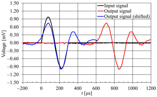
Figure 1.
Representation of the input and output signals in BE test.
Assuming homogeneous linear elastic material with known density , the can be calculated as:
Although the BE technique is widely used, signal interpretation remains a challenge, especially in the determination of [41,42,43]. There are several methods to determine , which can be categorized into two main groups: time domain methods (arrival-to-future, peak-to-peak and cross-correlation methods) and frequency domain methods (discrete and continuous methods) [41]. Each of these methods has its own advantages and limitations, and there is currently no method for interpreting BE test results that has been clearly shown to be better than others [44]. As there is no clear approach for determining , the results obtained with BE are subject to a considerable degree of uncertainty and subjectivity [42]. However, time-domain methods are generally simpler and more straightforward, as can be determined directly by analyzing the time interval between specific points in the transmitted and received waveforms [14].
In this study, the peak-to-peak method was used to determine , as it gave better agreement with the results of the RC test (Figure 2). In contrast, the start-to-start method consistently yielded slightly shorter or higher , which is close to the results reported by Sas et al. [45]. Given the larger specimen size (), we also investigated the possible effects of wave attenuation as discussed by Gao et al. [43].
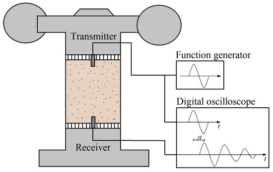
Figure 2.
Schematic representation of the BE setup in the RC device.
2.2. Resonant Column Test
The RC test device is the most commonly used laboratory device for determining and the material damping of soils in the range of between 10−6 and 10−3 (e.g., [46,47]).
The RC technique was originally developed in the 1930s by the Japanese engineers Ishimato and Iida [48]. It was further developed in the 1960s (e.g., [49,50,51]) and has since become a popular technique for studying the stress–strain response of soil. It is based on oscillation of a solid or hollow cylindrical specimen in one of its vibration modes (torsional, flexural and normal modes) to determine the resonant frequency. In general, RC devices can be divided into two groups: free-free and fixed-free [52]. In the free-free RC device, the actuator is attached to either the upper or lower end of the sample, while the other end remains free to rotate. In a fixed-free RC device, one side of the specimen is restricted in its rotation, while the other end with the mounted actuator is free to rotate. RC devices are often limited in their performance, as they are usually unable to measure a very small strain (down to without additional equipment [52].
In this study, the fixed-free torsional RC device from Wille Geotechnic was used (Figure 3); this device is capable of performing RC and BE tests simultaneously under isotropic and anisotropic stress conditions. The pneumatic system controls the cell and the back pressure up to 1000 kPa. To measure the axial deformation of the sample, the vertical displacement sensor is positioned in the confinement chamber. The volume changes during the saturation and consolidation stages are measured with a burette. The device works with sinusoidal torsional vibrations generated by two mini shakers attached to the top of the specimen, while the bottom of the specimen remains fixed. The force generated by the shakers is measured by a force sensor (excitation signal), while the movement of the sample is measured by an accelerometer (response signal) mounted on one side of the drive plate:
where is the root mean square RMS value of the response sensor voltage, is the RMS value of the excitation signal voltage, is the angular velocity, and is the frequency. Normally, the resonant frequency is determined by finding the maximum amplitude (e.g., [53]). Theoretically, this method is not applicable to larger strains when the soil has significant damping , since the resonant frequency is defined by a 90-degree phase shift between the response and the excitation (as shown in Figure 4 where the shift is applied to obtain a phase jump), and the frequency at maximum amplitude is:
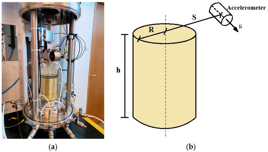
Figure 3.
(a) RC device setup. (b) Graphical representation of parameters estimating .
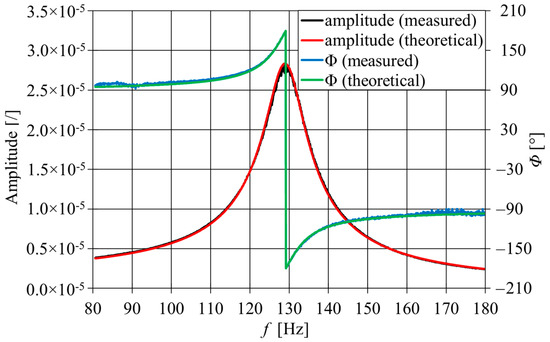
Figure 4.
An example of the frequency response curve.
The information required to calculate in the soil under the given conditions results from the resonant frequency , specimen height and boundary conditions defined by a factor [54]. Thus, can be calculated as:
The corresponding magnitude of engineering shear strain induced in a specimen can be calculated from the peak acceleration sensor amplitude at resonance , the accelerometer relative position and the specimen radius [54]. Thus, can be calculated as:
Typically, RC devices adhere to a 2:1 ratio between specimen height and diameter. However, this ratio can be adjusted to change the if there are limitations in the testing equipment or due to specific characteristics of the soil specimen [55].
3. Test Arrangement and Procedure
During the preparation stages, the soil samples were trimmed to produce cylindrical specimens with a final diameter of 70 mm. The height of the specimens, either 140 or 100 mm, was chosen considering the estimated effective stresses in situ and the consistency of the samples. For softer soil samples from shallower depths, problems were encountered with the performance of the mini oscillators at the lowest effective stress, particularly during oscillation with small shear stresses. To remedy this, the specimen height was adjusted to 100 mm to increase the resonant frequency and address the issues with the mini oscillators, following an approach similar to that of Kumar and Clayton [55]. The effect of specimen height on the measured was tested in advance to confirm the validity of the results on specimens with a lower height to diameter ratio.
Before and after testing, specimens were measured and weighed to determine water content and density [56,57]. Throughout the test, the vertical displacements of the specimen were measured using an internal transducer. The specimen volume was determined considering the final volume and the corresponding volume change during each consolidation stage. The specimen diameter was calculated assuming a perfect cylindrical shape, with constant radial strains over the entire height.
After inserting the specimen into the RC device, a low isotropic effective stress was applied, and the soil was saturated by increasing the back pressure. After the saturation stage, the vertical displacements were measured.
Each specimen was subjected to at least four consolidation stages, including isotropic and anisotropic conditions. In the first consolidation stage, an isotropic consolidation was performed in which the effective stress was set close to the horizontal stress under field conditions. The estimated coefficient of lateral earth pressure at rest was approximately 0.5 for all samples; therefore, to simplify the procedures, the value 0.5 was used for all tests. In the second consolidation phase, an isotropic consolidation was performed with an effective stress corresponding to the stress under field conditions. In the third consolidation stage, anisotropic consolidation was carried out with an effective vertical stress corresponding to the field conditions and a horizontal stress set at 0.5 times the effective vertical stress. In the fourth consolidation stage, a further isotropic consolidation was performed with an effective stress corresponding to the effective vertical stress under field conditions. To investigate the effect of the stress state on the stiffness at small strains, some specimens were subjected to additional isotropic consolidation stages with stresses 2 or 4 times higher than the fourth consolidation stage.
After each consolidation stage, both BE and RC tests were performed. The BE test was repeated three times with different frequencies of the transmitter (input signal) (black line in Figure 1). For each BE test, the transit time was determined, and then the shear modulus was calculated. The final result was calculated from the average of the three measurements. After the BE test, an RC test was carried out under undrained conditions. The excess pore water pressure during the vibrations was measured using a pore pressure transducer.
Unfortunately, BE tests could not be performed on all soil samples due to equipment problems. In the cases labelled RCBE in Table 2, both BE and RC tests were performed. In cases when only the RC test was performed, the sample is labelled RC.
Table 2.
Properties of soil and testing conditions.
4. Materials
For this analysis, cohesive soil samples were taken from a site in Škofljica on the periphery of the Ljubljana Marsh. The soft lacustrine sediments at the site are cohesive soils (), predominantly clays of medium to high plasticity with up to 39% fine sand [58] and a between 11 and 35% according to Atterberg limits [59]. A total of 45 BE tests and 89 RC tests were carried out on 20 soil samples under different stress conditions. The influence of sample size was also considered in the study.
5. Test Results and Discussion
To illustrate the test results, sample RCBE_10 is examined in detail. Figure 5a shows the test results for all four consolidation stages. As expected, increases with increasing effective stress. However, under anisotropic stress conditions, a marginal increase in can be observed for the same . This tendency can be observed in the BE and RC tests. The increase in may be the result of anisotropic stress conditions or a slight decrease in due to anisotropic loading stage (consolidation and creep).
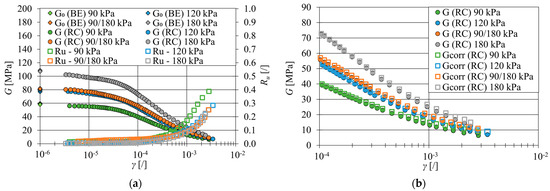
Figure 5.
(a) The test results of the RC and BE tests of sample RC_10 for all consolidation stages (b) Correction of due to .
The induced by RC vibrations reduces the effective stresses at which the test is performed. Similarly to liquefaction studies, is expressed as [60]:
where is the initial horizontal effective stress (after consolidation stage). Based on the HSS model, the corrected value of was calculated assuming kPa:
where is the horizontal effective stress during test, is the friction angle, and is the parameter determined from the results of the tests performed, which is approximately 0.7. As shown in Figure 5b, leads to a negligible degradation of in the strain range up to 7.0 × 10⁻⁴. This correction agrees well with Hsu and Vucetic [61], who proposed a low threshold for strength reduction due to for silts and clays with a between 14 and 30%, where is between 2.4 × 10⁻⁴ and 6.0 × 10⁻⁴. Only at larger strains is some degradation of due to observed.
5.1. Influence of Sample Size
As mentioned above, the RC device encountered some problems when testing softer soil samples at low stresses. Therefore, the sample heights were selected in a range from 140 mm to 100 mm. The influence of sample height was investigated using sample RC_20. The initial height of the specimen was 140 mm (height/diameter ratio 2:1). After the isotropic final consolidation stage (), the specimen was shortened to 100 mm (height/diameter ratio 1.4:1) and consolidated again under the same effective stress. As can be seen in Figure 6, almost no differences were observed between for the two specimen heights along the entire shear strain range.
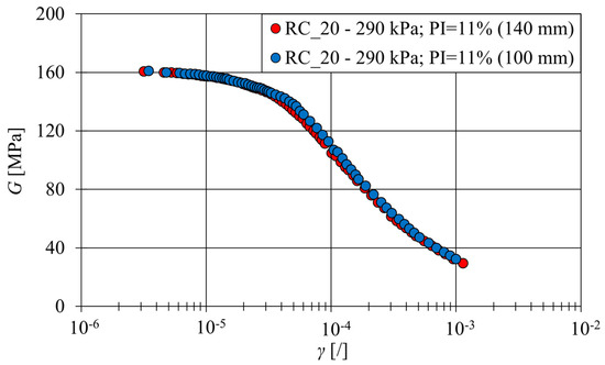
Figure 6.
The results of the RC test performed on a 140 and 100 mm high specimen.
The possible influence of wave attenuation [43] on the determination of from the BE test results was investigated using sample RCBE_6. After the isotropic final consolidation stage (), the specimen was shortened from the initial height of 110 mm to 90 mm, 70 mm and 50 mm and consolidated again with the same effective stress. For each specimen height, the BE tests were repeated at three different frequencies of the transmitted signal. The results in Figure 7 show that there are no significant differences in for different specimen heights. The differences in for each of the three measurements are more pronounced for shorter samples and are probably due to the accuracy of the transit time determination. However, the differences between the lowest and highest measured are 2.5% and reflect 5.9% differences between the determined. Using the average value of , the difference between the determined is reduced to only 1%.
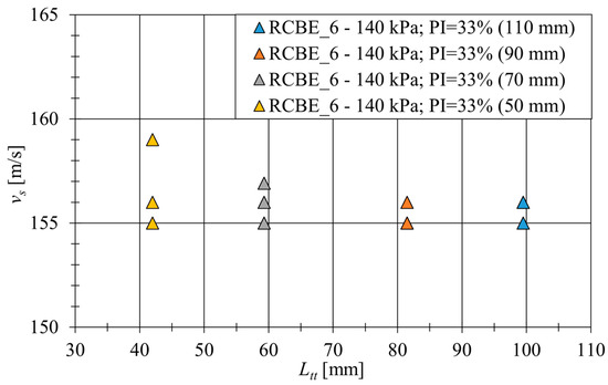
Figure 7.
The results of the BE test on RCBE_6 sample for different .
5.2. G Measurements
As already mentioned, limitations of the RC device exist, as the measurements cannot reach very small strains (. Figure 8a shows that there is no pronounced constant for soils with low plasticity, but that they increase slightly with decreasing . In contrast, soils with higher plasticity in Figure 8b tend to have constant at .
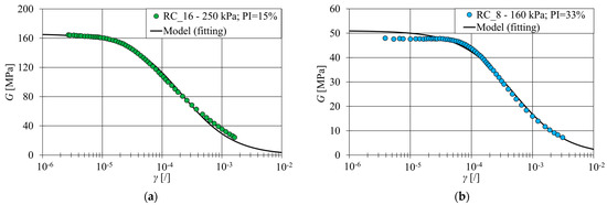
Figure 8.
Example of fitting the modified Hardin–Drnevich model: curves for a specimen (a) with low and (b) with high .
In RC experiments, the highest measured can be regarded as . However, to minimize the effects of measurement errors, it may be more appropriate to fit the measurements to the modified Hardin–Drnevich (Equation (2)) model, as shown in Figure 8. This leads to a slightly higher estimate of . The comparison between and resulting from fitting the modified Hardin–Drnevich model shows that is consistently about 10% lower than fitted regardless of the isotropic or anisotropic stress conditions (Figure 9).
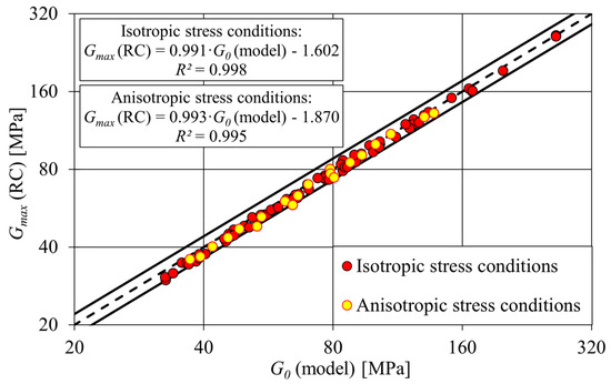
Figure 9.
Comparison between (model) and (RC), where solid black lines lay ± 10% from identity line.
The measurements with the BE test could be compared with the modified Hardin–Drnevich model, which was adapted to the measurements with the RC test (Figure 10). The results show that there can be a difference of about ±10% between the determined with the BE test and the resulting from the fit of the modified Hardin–Drnevich model. Only at two data points is there a discrepancy between the BE and RC measurements of more than 10%, the cause of which is not immediately apparent. In addition, these two outliers were subsequently excluded from the regression analysis. There were also no significant differences under anisotropic stress conditions.
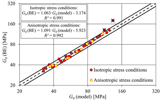
Figure 10.
Comparison between (model) and (BE), where the solid black lines are ±10% away from the identity line. Two outliers that were excluded from regression analysis are marked with X.
5.3. G/G0 Curves
In practice, can be measured in situ, while laboratory measurements are used to determine the and curves. In this study, the curves were determined using best-fit parameters according to the modified Hardin–Drnevich model. The results of the model fitting are the parameters and . Figure 11 shows the curves for all 20 samples (Table 2) tested under different stress conditions.
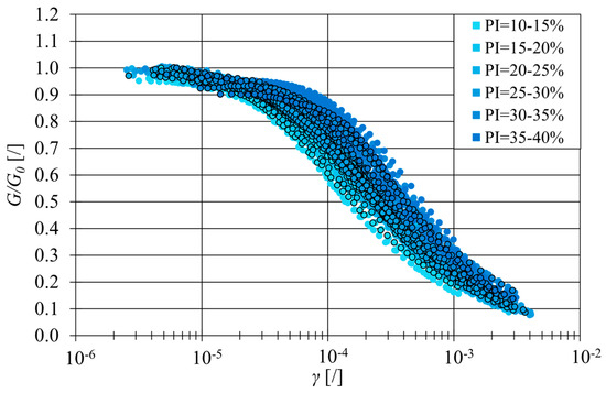
Figure 11.
for all soil samples under different stress conditions. The circles outlined in black are test results performed under anisotropic stress conditions.
The modified Hardin–Drnevich model was originally developed and tested primarily for sandy soils [62]. Figure 12 shows that soil with a matches the model almost perfectly, while soil with a shows a more pronounced plateau in the range of smaller than 5 × 10⁻⁵. Better agreement can be achieved if the power factor coefficient is included (Equation (3)), as recommended by Stokoe [27]. However, such a formulation of the hyperbolic model is not included in the HSS model.
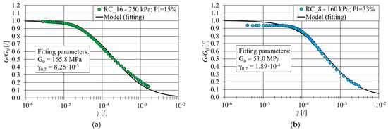
Figure 12.
Example of fitting modified Hardin–Drnevich model: curves for a specimen (a) with low and (b) with high .
The comparison between the established empirical models (Table 1) and measurements (Figure 13) is presented in this study in the form of . The empirical curves for different were also fitted according to the modified Hardin–Drnevich model to determine , and then exponential trend lines were generated for each model (Figure 13). Both the empirical curves and the measurements show that increases with . However, discrepancies in the exist not only between the empirical curves and the measurements, but also between the empirical curves of different authors. When analyzing the results in Figure 13, the empirical models of Darendeli [22], Zhang et al. [30] and Ciancimino et al. [31], which also take into account, show that the influence of is less pronounced compared to the other models (the slope of the line is less steep). It can be seen from the measurement results that the results for the local soils can deviate from the general equations in the literature.
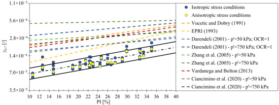
Figure 13.
The comparison between the empirical models and the measurements represented by γ0.7, with the black lines deviating ±25% from the trend [17,22,29,30,31].
This study also confirms that should not be completely neglected in relation to . In the cases where only four consolidation stages were measured, there was no significant increase in with . This could be due to random measurement errors or other influences on . To further investigate the effect of stress state on stiffness at small strains, some specimens were subjected to additional isotropic consolidation stages with stresses 2 or 4 times higher than those of the fourth consolidation stage. The result was a significant increase in (Figure 14). It was also found that anisotropic stress conditions did not significantly change . Isotropic and anisotropic tests at the same (second lowest ) are so close to each other in Figure 14 that they can hardly be distinguished. Comparing measurements with the empirical model of Darendeli [22] and Zhang et al. [30], a comparable increase in can be observed. A comparison shows that the empirical model proposed by Ciancimino et al. [31] has a less pronounced influence of for soils with higher , as the lines are less steep.
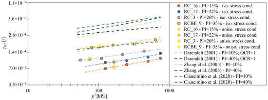
Figure 14.
The comparison of increase in with between the empirical models and the measurements [22,30,31].
6. Conclusions
This article presents the first measurements of the shear modulus at small strains of the soft lacustrine sediments of the Ljubljana Marsh. The extensive laboratory program included 45 bender element (BE) and 89 resonant column (RC) tests on cohesive soils with between 11% and 35%. This study not only compared these measurements with widely used empirical relationships, but also investigated the effects of stress anisotropy on soil stiffness at small strains. In addition, the influence of soil sample softness and/or equipment limitations was also investigated in this study. For effective soil modeling, it is important to know the limitations of the equipment used. This knowledge is crucial for determining the necessary parameters for the implementation of the HSS model. These measurements play an important role in the development of the built environment in the Ljubljana Marsh. The main conclusions of this study are summarized below:
- , measured with BE, is slightly higher than , measured with RC. The reason for this is that RC was not able to measure at , which is also in agreement with Schaeffer et al. [52]. When the measurements were extended according to the modified Hardin–Drnevich model, both (BE) and (model) were within 10% of each other. In addition, the integration of the BE into the RC device facilitates the quality control of the measurements and thus increases the confidence in the measurement results.
- For the BE test, no significant influence of specimen height on the was found in this study. It was also found that for the RC test, shortening the specimen height to 1.4 times the diameter had no significant effect on the measured and the curve.
- Corrections of due to for these soft soils are not absolutely necessary. The range of in which developed in our experiments is similar to the results of Hsu and Vucetic [61].
- It was found that was dependent on and . Trends similar to those of the empirical models were observed, with the exception that was lower than the value reported by other authors. However, large differences were also found between the empirical models. Apparently, there is no universally valid empirical model for the prediction of the curve, as reported by Sobol et al. [19]. It is, therefore, recommended to perform measurements on local soils, especially in cases where the validity of the empirical relationships has not yet been confirmed.
- and at the same were comparable for isotropic and anisotropic stress conditions, indicating that there is no significant influence of the anisotropic stress conditions on the curve for this cohesive soil.
- It can be seen that both isotropic and anisotropic tests led to an approximately equal curve if the test was performed at a stress state close to the field value of . Testing at significantly higher or lower led to different . To obtain reliable shear modulus values at small strains, the tests should, therefore, be performed close to the field conditions.
Author Contributions
Conceptualization, T.J., B.P. and M.M.; methodology T.J., B.P. and M.M.; investigation T.J.; writing—original draft preparation T.J.; writing—review and editing T.J., B.P. and M.M.; visualization T.J. and M.M.; supervision B.P. and M.M. All authors have read and agreed to the published version of the manuscript.
Funding
This research was funded by the Slovenian Research Agency (research core funding No. P2-0180) within Young Researcher program.
Institutional Review Board Statement
Not applicable.
Informed Consent Statement
Not applicable.
Data Availability Statement
Data is contained within the article.
Acknowledgments
The authors gratefully acknowledge the financial support provided by the Slovenian Research Agency and Matjaž Mikoš, the head of the research group. Special thanks are extended to Alessandro Flora, Lucia Mele, and Roberta Ventini from the University of Naples Federico II for their valuable contributions to this research.
Conflicts of Interest
The authors declare no conflicts of interest.
References
- Gaberc, A. Napovedano in opazovano posedanje Južne obvoznice. In Proceedings of the 1st Šuklje Symposium, Ljubljana, Slovenia, 12 October 2000; Gaberc, A.M., Majes, B., Eds.; Slovenian Geotechnical Society: Ljubljana, Slovenia, 2000; pp. 121–128. [Google Scholar]
- Mencej, Z. Prodni Zasipi pod Jezerskimi Sedimenti Ljubljanskega Barja. Geologija 1980, 31–32, 517–533. [Google Scholar]
- Jardine, R.J.; Potts, D.M.; Fourie, A.B.; Burland, J.B. Studies of the Influence of Non-Linear Stress–Strain Characteristics in Soil–Structure Interaction. Géotechnique 1986, 36, 377–396. [Google Scholar] [CrossRef]
- Burland, J.B. Ninth Laurits Bjerrum Memorial Lecture: “Small Is Beautiful”—The Stiffness of Soils at Small Strains. Can. Geotech. J. 1989, 26, 499–516. [Google Scholar] [CrossRef]
- Schanz, T.; Vermeer, P.A.; Bonnier, P.G. The hardening soil model: Formulation and verification. In Beyond 2000 in Computational Geotechnics; Routledge: London, UK, 2019; pp. 281–296. ISBN 1315138204. [Google Scholar]
- Benz, T. Small-Strain Stiffness of Soils and Its Numerical Consequences. Ph.D. Thesis, University of Stuttgart, Stuttgart, Germany, 2007. [Google Scholar]
- Obrzud, R.F. On the Use of the Hardening Soil Small Strain Model in Geotechnical Practice. Numer. Geotech. Struct. 2010, 16, 1–17. [Google Scholar]
- Wong, J.K.H.; Wong, S.Y.; Wong, K.Y. Extended Model of Shear Modulus Reduction for Cohesive Soils. Acta Geotech. 2022, 17, 2347–2363. [Google Scholar] [CrossRef]
- Kishida, T. Comparison and Correction of Modulus Reduction Models for Clays and Silts. J. Geotech. Geoenviron. Eng. 2017, 143, 04016110. [Google Scholar] [CrossRef]
- Ferreira, C.; Viana da Fonseca, A.; Santos, J.A. Comparison of Simultaneous Bender Elements and Resonant Column Tests on Porto Residual Soil. In Soil Stress-Strain Behavior: Measurement, Modeling and Analysis, Proceedings of the Geotechnical Symposium in Rome, Italy, 16–17 March 2006; Ling, H.I., Callisto, L., Leshchinsky, D., Koseki, J., Eds.; Solid Mechanics and Its Applications; Springer: Dordrecht, The Netherlands, 2007; Volume 146, pp. 523–535. ISBN 978-1-4020-6145-5. [Google Scholar]
- Camacho-Tauta, J.; Santos, J.A.; Fonseca, A.V. Two Bender Receivers Frequency Domain Analysis in Resonant Column Tests. In Advances in Soil Dynamics and Foundation Engineering, Geotechnical Special Publication 240; Society of Civil Engineers: New York, NY, USA, 2014; pp. 72–82. [Google Scholar]
- Camacho-Tauta, J.; Cascante, G.; Santos, J.A. Measurements of Shear Wave Velocity by Resonant-Column Test, Bender Element Test and Miniature Accelerometers. In Proceedings of the Pan-Am CGS Geotechnical Conference; Canadian Geotechnical Society: Richmond, BC, Canada, 2001; Volume 949, pp. 1–9. [Google Scholar]
- Pereira, C.; Correia, A.G.; Ferreira, C.; Santos, J.; Santos, J. Measurement of Shear Modulus Using Bender Elements and Resonant-Column. In Fundamentals to Applications in Geotechnics, Proceedings of the 15th Pan-Am Conference on Soil Mechanics and Geotechnical Engineering, 15–18 November 2015; IOS Press: Buenos Aires, Argentina, 2015; pp. 120–129. [Google Scholar] [CrossRef]
- Sas, W.; Gabryś, K.; Szymański, A. Comparison of resonant column and Bender elements tests on selected cohesive soil from Warsaw. Electron. J. Pol. Agric. Univ. EJPAU 2014, 17, 7. Available online: http://www.ejpau.media.pl/volume17/issue3/art-07.html (accessed on 23 July 2014).
- Clayton, C.R.I. Stiffness at Small Strain: Research and Practice. Géotechnique 2011, 61, 5–37. [Google Scholar] [CrossRef]
- Hardin, B.O.; Black, W.L. Vibration Modulus of Normally Consolidated Clay. J. Soil Mech. Found. Div. 1968, 94, 353–369. [Google Scholar] [CrossRef]
- Vucetic, M.; Dobry, R. Effect of Soil Plasticity on Cyclic Response. J. Geotech. Eng. 1991, 117, 89–107. [Google Scholar] [CrossRef]
- Presti, L. Estimate of Elastic Shear Modulus in Holocene Soil Deposits. Soils Found. 1998, 38, 263–265. [Google Scholar]
- Soból, E.; Gabryś, K.; Zabłocka, K.; Šadzevičius, R.; Skominas, R.; Sas, W. Laboratory Studies of Small Strain Stiffness and Modulus Degradation of Warsaw Mineral Cohesive Soils. Minerals 2020, 10, 1127. [Google Scholar] [CrossRef]
- Sun, J.; Golesorkhi, R.; See, H. Dynamic Moduli and Damping Ratio for Cohesive Soils; Report No. UCB/EERC-88/15; University of California Berkeley-Earthquake Engineering Research Center: Berkeley, CA, USA, 1988; 42p. [Google Scholar]
- Hardin, B.O.; Drnevich, V.P. Shear Modulus and Damping in Soils: Design Equations and Curves. J. Soil Mech. Found. Div. 1972, 98, 667–692. [Google Scholar] [CrossRef]
- Darendeli, M. Development of a New Family of Normalized Modulus Reduction and Material Damping Curves. Ph.D. Thesis, University of Texas, Austin, TX, USA, 2001. [Google Scholar]
- Santos, J.A.; Correia, A.G. Reference threshold shear strain of soil, its application to obtain a unique strain-dependent shear modulus curve for soil. In Proceedings of the 15th International Conference on Soil Mechanics and Geotechnical Engineering, Istanbul, Turkey, 27–31 August 2001; pp. 267–270. [Google Scholar]
- Ishibashi, I.; Zhang, X. Unified Dynamic Shear Moduli and Damping Ratios of Sand and Clay. Soils Found. 1993, 33, 182–191. [Google Scholar] [CrossRef]
- Lanzo, G.; Vucetic, M.; Doroudian, M. Reduction of Shear Modulus at Small Strains in Simple Shear. J. Geotech. Geoenviron. Eng. 1997, 123, 1035–1042. [Google Scholar] [CrossRef]
- Kokusho, T.; Yoshida, Y.; Esashi, Y. Dynamic Properties of Soft Clay for Wide Strain Range. Soils Found. 1982, 22, 1–18. [Google Scholar] [CrossRef] [PubMed]
- Stokoe, K.H.; Darendeli, M.B.; Andrus, R.D.; Brown, L.T. Dynamic soil properties: Laboratory, field and correlation studies. In Earthquake Geotechnical Engineering; A A Balkema: Rotterdam/Brookfield, The Netherlands, 1999; pp. 811–845. [Google Scholar]
- Vardanega, P.J.; Bolton, M.D. Stiffness of Clays and Silts: Normalizing Shear Modulus and Shear Strain. J. Geotech. Geoenviron. Eng. 2013, 139, 1575–1589. [Google Scholar] [CrossRef]
- Electric Power Research Institute—EPRI. Guidelines for Determining Design Basis Ground Motions; Report EPRI TR-102293; EPRI: Palo Alto, CA, USA, 1993. [Google Scholar]
- Zhang, J.; Andrus, R.D.; Juang, C.H. Normalized Shear Modulus and Material Damping Ratio Relationships. J. Geotech. Geoenviron. Eng. 2005, 131, 453–464. [Google Scholar] [CrossRef]
- Ciancimino, A.; Lanzo, G.; Alleanza, G.A.; Amoroso, S.; Bardotti, R.; Biondi, G.; Cascone, E.; Castelli, F.; Di Giulio, A.; d’Onofrio, A.; et al. Dynamic Characterization of Fine-Grained Soils in Central Italy by Laboratory Testing. Bull. Earthq. Eng. 2020, 18, 5503–5531. [Google Scholar] [CrossRef]
- Stokoe, K.H.; Hwang, S.K.; Darendeli, M.B.; Lee, N.J. Correlation Study of Nonlinear Dynamic Soils Properties; Westinghouse Savannah River Co.: Aiken, SC, USA, 1995. [Google Scholar]
- Payan, M.; Chenari, R.J. Small Strain Shear Modulus of Anisotropically Loaded Sands. Soil Dyn. Earthq. Eng. 2019, 125, 105726. [Google Scholar] [CrossRef]
- Jafarian, Y.; Javdanian, H. Small-Strain Dynamic Properties of Siliceous-Carbonate Sand under Stress Anisotropy. Soil Dyn. Earthq. Eng. 2020, 131, 106045. [Google Scholar] [CrossRef]
- Goudarzy, M.; Magnanimo, V.; König, D.; Schanz, T. Anisotropic Stress State and Small Strain Stiffness in Granular Materials: RC Experiments and DEM Simulations. Meccanica 2020, 55, 1869–1883. [Google Scholar] [CrossRef]
- Pennington, D.S.; Nash, D.F.T.; Lings, M.L. Anisotropy of G0 Shear Stiffness in Gault Clay. Géotechnique 1997, 47, 391–398. [Google Scholar] [CrossRef]
- Hao, G.L.; Lok, T.M.H. Study of Shear Wave Velocity of Macao Marine Clay under Anisotropic Stress Condition. In Proceedings of the 14 World Conference on Earthquake Engineering, Beijing, China, 12–17 October 2008. [Google Scholar]
- Shirley, D.J.; Hampton, L.D. Shear-wave Measurements in Laboratory Sediments. J. Acoust. Soc. Am. 1978, 63, 607–613. [Google Scholar] [CrossRef]
- Dyvik, R.; Olsen, T.S. Gmax measured in oedometer and DSS tests using bender elements. In Proceedings of the 12th International Conference on Soil Mechanics and Foundation Engineering, ICSMFE 1989, Rio de Janeiro, Brazil, 13–18 August 1989; Publications Committee of XII ICSMFE, Ed.; Taylor & Francis: Milton Park, UK, 1989; Volume 1, pp. 39–42. [Google Scholar]
- Jovičić, V.; Coop, M.P. The Measurement of Stiffness Anisotropy in Clays with Bender Element Tests in the Triaxial Apparatus. Geotech. Test. J. 1998, 21, 3–10. [Google Scholar] [CrossRef]
- Wang, Y.; Benahmed, N.; Cui, Y.-J.; Tang, A.M. A Novel Method for Determining the Small-Strain Shear Modulus of Soil Using the Bender Elements Technique. Can. Geotech. J. 2017, 54, 280–289. [Google Scholar] [CrossRef]
- Ingale, R.; Patel, A.; Mandal, A. Performance Analysis of Piezoceramic Elements in Soil: A Review. Sens. Actuators Phys. 2017, 262, 46–63. [Google Scholar] [CrossRef]
- Gao, Y.; Zheng, X.; Wang, H.; Luo, W. Effect of Wave Attenuation on Shear Wave Velocity Determination Using Bender Element Tests. Sensors 2022, 22, 1263. [Google Scholar] [CrossRef] [PubMed]
- Yamashita, S.; Kawaguchi, T.; Nakata, Y.; Mikami, T.; Fujiwara, T.; Shibuya, S. Interpretation of International Parallel Test on the Measurement of Gmax Using Bender Elements. Soils Found. 2009, 49, 631–650. [Google Scholar] [CrossRef]
- Sas, W.; Gabryś, K.; Soból, E.; Szymański, A. Dynamic Characterization of Cohesive Material Based on Wave Velocity Measurements. Appl. Sci. 2016, 6, 49. [Google Scholar] [CrossRef]
- Stokoe II, K.H.; Lodde, P.F. Dynamic Response of San Francisco Bay Mud. In From Volume I of Earthquake Engineering and Soil Dynamics, Proceedings of the ASCE Geotechnical Engineering Division Specialty Conference, Pasadena, CA, USA, 19–21 June 1978; Sponsored by Geotechnical Engineering Division of ASCE in Cooperation with; American Society of Civil Engineers: New York, NY, USA, 1978; Volume 2, pp. 940–959. [Google Scholar]
- Lai, C.G. Simultaneous Inversion of Rayleigh Phase Velocity and Attenuation for Near-Surface Site Characterization; Georgia Institute of Technology: Atlanta, GA, USA, 1998. [Google Scholar]
- Ishimoto, M.; Iida, K. Determination of Elastic Constants of Soils by Means of Vibration Methods; Bulletin of the Earthquake Research Institute: Tokyo, Japan, 1937; Volume 15, 67p. [Google Scholar]
- Hall, J.R.; Richart, F.E. Dissipation of Elastic Wave Energy in Granular Soils. J. Soil Mech. Found. Div. 1963, 89, 27–56. [Google Scholar] [CrossRef]
- Hardin, B.O.; Music, J. Apparatus for Vibration of Soil Specimens During Triaxial Test. In Apparatus for Vibration of Soil Specimens During the Triaxial Test; ASTM International: West Conshohocken, PA, USA, 1965; Volume 436, pp. 55–74. [Google Scholar]
- Drnevich, V.P. Effects of Strain History on the Dynamic Properties of Sand. Ph.D. Thesis, University of Michigan, Ann Arbor, MI, USA, 1967. [Google Scholar]
- Schaeffer, K.; Bearce, R.; Wang, J. Dynamic Modulus and Damping Ratio Measurements from Free-Free Resonance and Fixed-Free Resonant Column Procedures. J. Geotech. Geoenviron. Eng. 2013, 139, 2145–2155. [Google Scholar] [CrossRef]
- Gabrys, K.; Sobol, E.; Markowska-Lech, K.; Szymański, A. Shear Modulus of Compacted Sandy Clay from Various Laboratory Methods. IOP Conf. Ser. Mater. Sci. Eng. 2019, 471, 042022. [Google Scholar] [CrossRef]
- Wichtmann, T.; Sonntag, T.; Triantafyllidis, T. Über das Erinnerungsvermögen von Sand unter zyklischer Belastung. Bautechnik 2001, 78, 852–865. [Google Scholar] [CrossRef]
- Kumar, J.; Clayton, C.R. Effect of Sample Torsional Stiffness on Resonant Column Test Results. Can. Geotech. J. 2007, 44, 221–230. [Google Scholar] [CrossRef]
- ISO 17892-1:2014; Geotechnical Investigation and Testing—Laboratory Testing of Soil—Part 1: Determination of Water Content. European Commission for Standardization: Brussels, Belgium, 2014.
- ISO 17892-2:2014; Geotechnical Investigation and Testing—Laboratory Testing of Soil—Part 2: Determination of Bulk Density. European Commission for Standardization: Brussels, Belgium, 2014.
- ISO 114688-2:2017; Geotechnical Investigation and Testing—Identification and Classification of Soil—Part 2: Principles for a Classification. ISO copyright office: Geneva, Switzerland, 2017.
- ISO 17892-12:2018; Geotechnical Investigation and Testing—Laboratory Testing of Soil—Part 12: Determination of Liquid and Plastic Limits. European Commission for Standardization: Brussels, Belgium, 2014.
- Kramer, S. Performance-based design methodologies for geotechnical earthquake engineering. Bull. Earthq. Eng. 2013, 12, 1049–1070. [Google Scholar] [CrossRef]
- Hsu, C.-C.; Vucetic, M. Threshold Shear Strain for Cyclic Pore-Water Pressure in Cohesive Soils. J. Geotech. Geoenviron. Eng. 2006, 132, 1325–1335. [Google Scholar] [CrossRef]
- Brinkgreve, R.; Engin, E.; Engin, H.K. Validation of Empirical Formulas to Derive Model Parameters for Sands. In Numerical Methods in Geotechnical Engineering; Taylor & Francis Group: London, UK, 2010; ISBN 978-0-415-59239-0. [Google Scholar]
Disclaimer/Publisher’s Note: The statements, opinions and data contained in all publications are solely those of the individual author(s) and contributor(s) and not of MDPI and/or the editor(s). MDPI and/or the editor(s) disclaim responsibility for any injury to people or property resulting from any ideas, methods, instructions or products referred to in the content. |
© 2024 by the authors. Licensee MDPI, Basel, Switzerland. This article is an open access article distributed under the terms and conditions of the Creative Commons Attribution (CC BY) license (https://creativecommons.org/licenses/by/4.0/).