1. Introduction
Rural roads constitute an integral part of the roadway network providing vital access to rural towns and communities (including farms and ranches). According to the fatality facts 2021, around 40% of traffic fatalities took place in rural areas, although only 20% of people in the U.S. live there, and 32% of all vehicle miles traveled (VMT) occurred in rural areas [
1]. These statistics demonstrate the need for improving rural road safety and the requirement to effectively include it in the ongoing state safety improvement programs.
Network screening is the first step of highway safety improvement programs (HSIPs) which involve the identification of sites with potential for safety improvement on the roadway network. The resulting list of identified sites are given priority for detailed engineering studies to identify crash patterns, contributing factors, and potential countermeasures [
2,
3]. Errors in ranking the sites may produce a large number of false negatives (i.e., sites needing safety improvement mistakenly considered as safe) and a large number of false positives (i.e., truly safe sites identified as needing safety improvement). These errors result in an inefficient use of the resources dedicated to safety improvements and eventually reduce the overall effectiveness of the safety management programs. Therefore, the correct identification of safety improvement sites is essential for the successful implementation of any highway safety program.
Most traditional network screening methods rely on the crash frequency, crash rate, crash severity, or any combination of these measures [
4,
5]. Most of the existing ranking techniques for identifying safety improvement sites are reactive in nature [
6], as they rely on crash data only [
7]. Thus, these techniques require crashes to occur before identifying the potential sites for safety improvement. On the other hand, several proactive approaches have been proposed and used that require detailed data on roadway geometry and roadside characteristics, besides crash and traffic data [
8]. A major challenge for network screening on rural roads is the lack of access to the required crash, roadway, and traffic data at the network level especially for roadways that are owned and operated by local agencies.
This research seeks to evaluate the performance of a new, yet simplistic approach for network screening that was tailored for use on rural roadways [
9]. The proposed method requires minimal data for implementation, which could be valuable for agencies having limited access to detailed databases or extensive technical expertise.
2. Background
Numerous network screening techniques have been used in practice or proposed in the literature with each having its own strengths and limitations. Compared with the large number of studies focused on the development of various hotspot identifications methods, considerably less research has been dedicated to evaluating the performance of various methods [
10]. In this section, the major studies that evaluated the performance of different network screening techniques are summarized and presented. The Empirical Bayes estimate obtained from the EB method is the weighted sum of the expected value and the actual value, where the weights are determined based on the number of actual measurements for a certain variable. The potential for safety improvements (PSI) is estimated as the difference between the EB expected number of crashes and the predicted number of crashes found from the respective using safety performance function (SPF). A segment is said to have potential for improvement if the observed number of crashes is greater than the predicted number of crashes for that segment.
Kwon et al. [
11] examined the performance of three network screening methods for identifying potential sites for safety improvements on highways. The three network screening methods are Sliding Moving Window (SMW), Peak Searching (PS), and Continuous Risk Profile (CRP). The crash data from segmented sites were used to calculate the excess expected average crash frequency using Empirical Bayes adjustment based on two distinct sets of Safety Performance Functions (SPFs). These estimations from each approach were subsequently used to prioritize sites for safety investigations, comparing them against confirmed high crash location. The results revealed that the CRP method demonstrated the least occurrence of false positives, effectively identifying sites warranting safety investigations.
A study by Ambrose et al. [
12] investigated the difference between network screening results based on multivariate and simple crash prediction models. This study first compared the list of segments using Spearman’s rank correlation coefficient between the two models. Secondly, this study assessed the equality of statistical distributions of potential for safety improvement (PSI) value, which was obtained as a difference between predicted crash frequency and EB estimate. The third comparison was the percentage of segments identified in both lists. The findings suggested that the results from both methods were comparable.
A study conducted in Brazil [
13] compared different safety performance measures and their practical limitations using a sample of signalized intersections located in Fortaleza City, Brazil. The safety performance measures evaluated in this study average crash frequency (ACF), crash rate (CR), Equivalent Property Damage Only (EPDO), Level of Service of Safety (LOSS), Excess Predicted Average Crash Frequency using Safety Performance Functions (SPFs), Expected Average Crash Frequency with EB Adjustments (EB), and Excess Expected Average Crash Frequency with EB Adjustment (EEB). The difference in rank between each safety performance measure assessed and the Excess Expected Average Crash Frequency with EB Adjustment (EEB) was used to evaluate the performance of the subjected method. The findings suggested that the most comprehensive measure was EEB, and that fundamental measures like crash frequency and crash rate displayed reasonably similar rankings.
The effectiveness of several network screening techniques was examined in an Italian study [
14] using a set of criteria. These included reliability in detecting hazardous sites over a period, efficiency in finding sites with poor safety performance, and consistency in ranking. The potential for improvements (PFI) was examined along with the crash frequency, equivalent property damage only (EPDO), crash rate, proportion method, and EB estimates for total and severe crashes. This analysis used crash data from an Italian highway and found that the EB method outperformed all other approaches investigated in this study.
A study conducted by the Federal Highway Administration (FHWA) [
15] evaluated four methods of network screening aimed at identifying areas with the highest potential for safety enhancements. The methods evaluated in this study are crash frequency, crash rate, EB expected crashes, and EB excess expected crashes, considering both fatal and non-fatal injury severity levels. The study involves the safety management process from network screening to economic analysis using the intersection data from New Hampshire. This study analyzed the overall economic benefit and benefit–cost ratio for each of the four techniques. The study findings revealed that the EB excess expected measure produce the list of sites with most significant economic benefit and the highest return on investment was generated using the EB expected measure.
Elvik [
16] conducted review of current methodologies for identifying safety improvement sites on roadways. The study findings concluded that the Empirical Bayes (EB) method is the most reliable method for network screening. Furthermore, through simulation experiments [
10] and the application of innovative robust evaluation criteria [
17], Cheng and Washington demonstrated that the EB method stands out as the most consistent and reliable technique for identifying sites with potential for safety improvements.
Although the EB method was found to better identify sites requiring safety improvement, it may be subject to several limitations under certain conditions, especially for local agencies. The EB method requires detailed data for roadway geometry and roadside characteristics besides technical expertise that is often inaccessible by local agencies (counties, towns, tribal governments, etc.).
3. Proposed Network Screening Approach: An Overview
This study validates a new network screening approach that was recently proposed for use on rural two-lane highways [
9]. The main merit of the proposed approach is that it can easily be implemented by local agencies lacking access to detailed databases and technical expertise. Specifically, the more sophisticated network screening methods (e.g., Empirical Bayes method) use exact values for various roadway characteristics (sometimes referred to as risk factors). While the use of exact values may improve the accuracy of the screening process, it requires access to extensive databases or on-site detailed measurements which are typically beyond the resources available for small local agencies. Hence, implementing such sophisticated methods might not be feasible for most local agencies. To minimize data requirements, the proposed approach employs classified variables that can easily be compiled by local agencies without the need to access detailed and extensive databases. Using the classified variables, the proposed method consists of regression models that are developed using the EB expected number of crashes to predict the level of risk (or safety) of roadway segments that are part of the roadway network. Two models were proposed, one with and one without traffic data. The response (dependent) variable in both models was the EB expected number of crashes, which is a function of the HSM predicted number of crashes and the observed number of crashes. The explanatory (independent) variables included roadway and roadside characteristics besides traffic exposure (AADT).
Table 1 shows the explanatory variables for the proposed models. The development of the mathematical model for this study using the proposed approach is discussed later in Section Model Development.
4. Study Area and Data Description
The two-lane rural road network in the state of Oregon was investigated as a case study in order to validate the proposed method. A total roadway segment sample of around 1495 miles from the eastern and western region was used in this investigation to ensure adequate geographic coverage. The study sample included roadways from different parts of the state as shown in
Figure 1. In general, roadways in the eastern part of the state run in flatter terrain with less restrictive alignment, while those in the western part of the state run in mountainous terrain with more restrictive alignment (winding routes, sharp radii, etc.).
All state-owned rural two-lane roads were identified using online geographic information system (GIS) data [
18]. The roadway segments were then selected from the collection to obtain sample data ensuring sufficient geographical coverage. Data were collected for roadway segments using 0.05-mile increments to ensure that data would capture all changes in the physical characteristics of the roadway, thus eliminating the possibility of missing significant differences between consecutive observation points. The posted speed limit in all the segments considered for this study is 55 mph. Intersections and 0.05-mile segments along upstream and downstream approaches were excluded from the dataset.
The Oregon Department of Transportation (DOT) online databases and video logs were used to identify and compile traffic, roadway geometry, roadside, and crash data [
19,
20]. The roadway geometric data includes lane width, shoulder type and width, horizontal curve presence degree of curvature, length of the horizontal curve, spiral curve presence and length, vertical curve presence and type, grade, and length of vertical curve. Roadside characteristics consists of driveway density, side slope ratings, and fixed object ratings. These two factors are taken from the Oregon DOT online database and video logs, respectively, both at 0.05-mile increment.
Crash data for ten years (2011–2020) were collected for the study sample using the Oregon DOT online database [
20]. Data on more than 20 individual crash characteristics- including crash location, road character, impact location, traffic control, crash type, crash severity, vehicle type, and weather condition were collected and combined with the geometric and roadside database forming an integrated dataset for analysis.
Traffic data from 2011 to 2020 were also collected separately and compiled to the study integrated dataset described earlier.
The study sample was shared with the Oregon DOT personnel to confirm that segments selected in the study sample did not undergo any major upgrade or improvement (including changes in speed limit) over the study period.
Segmentation
As mentioned earlier, the data was collected using 0.05-mile increments. Afterwards, the total sample was compiled into homogeneous segments concerning the following variables: annual average daily traffic (AADT), speed limit, lane and shoulder type and width, and roadside characteristics. Any change in these variables marked the end of a segment and the beginning of another segment.
Upon completing the segmentation, a total of 377 segments consisting of 1495 miles were compiled. Crash frequency data for two different periods (2011–2015, and 2016–2020) were compiled for roadway segments.
5. Methodology
The proposed approach was implemented using the study data and evaluated using observed crash history collected for the study sample. Specifically, the crash data collected over ten years were divided into two datasets: a training dataset spanning five years (2011–2015) to develop the regression model, and a testing dataset covering the subsequent five-year period (2016–2020). The approach that was used in evaluating the proposed network screening method is to compare site rankings using the proposed method with the respective rankings using crash history data. Both crash frequency and crash density (number of crashes per mile) were used in ranking sites. Further, rankings from the Empirical Bayes (EB) method and the potential for safety improvement (PSI) method were included in the analyses to see how the performance of the proposed method compares to that of the two well-established techniques. Using the EB and PSI in this study is based on the fact that these techniques has become the gold standard in performing quantitative safety analyses, with merits and effectiveness well established in the literature [
21,
22,
23,
24,
25,
26,
27].
Model Development
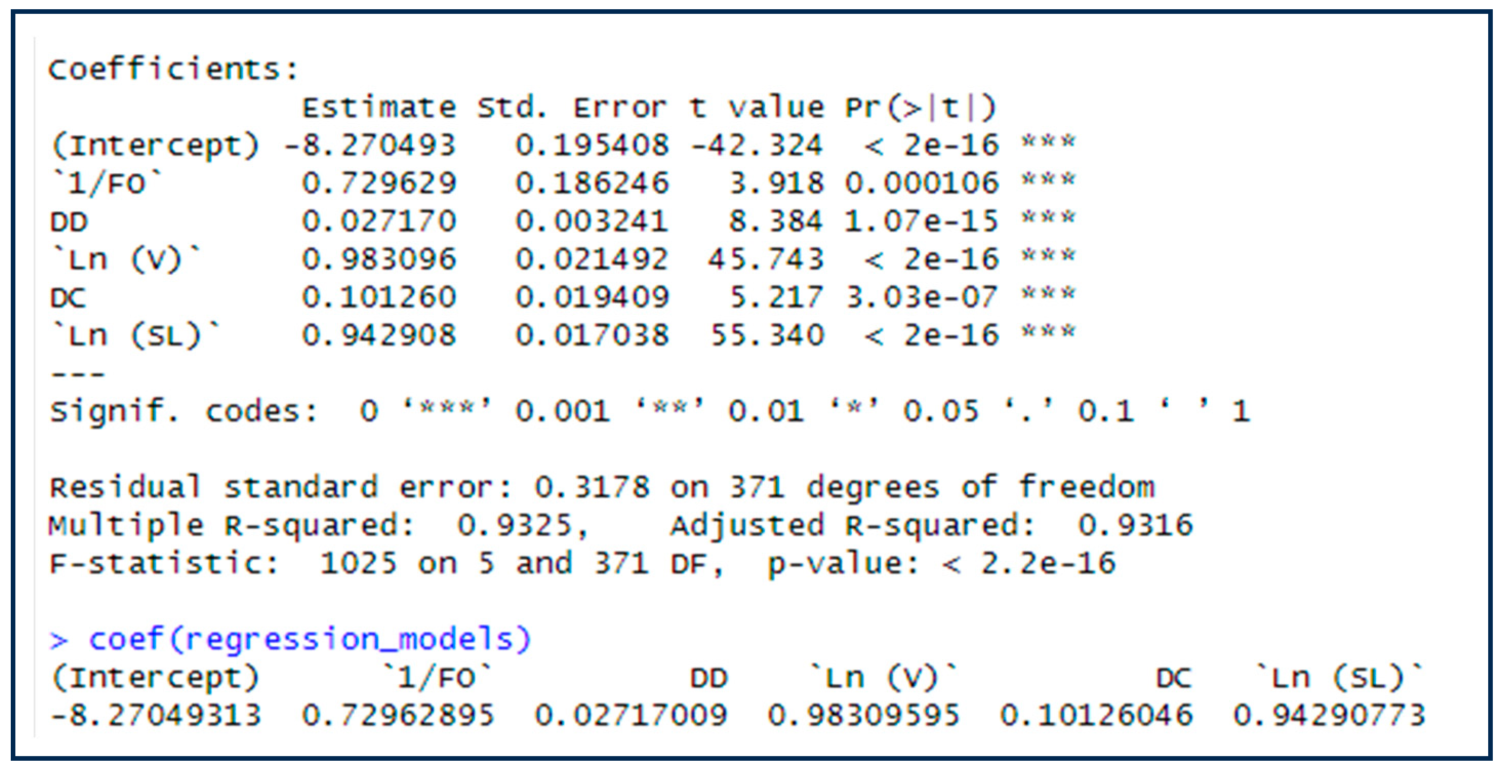
Multivariate linear regression analysis was used in developing the model for road network screening. The open-source statistical software R 4.3.1 was used for running the analysis. The model with different explanatory variables is shown in Equation (1).
where
exp = EB expected number of crashes per year;
SL = segment length in miles;
V = traffic volume (AADT);
FO = fixed object;
DD = driveway density; and
DC = degree of curvature.
This model has a coefficient of determination (adjusted R-squared value) of 0.932. This indicates that the model can explain about 93 percent of the variability of the EB expected number of crashes, which is relatively high given the classified format used for most of the variables in this model. All variable coefficients are found significant at the 95% confidence level. The regression output using R 4.3.1 statistical software is shown in
Figure 2.
6. Study Analysis and Results
This section presents the discussion of the metrics used for the evaluation of the performance of the proposed method. The performance of the EB method and the PSI method is also calculated and compared with the proposed method.
6.1. Spearman Correlation Coefficient
Initially, the Spearman’s rank correlation coefficient was calculated between the proposed method’s ranking and the ranking using observed crash data. The Spearman rank correlation coefficient is a nonparametric technique that is usually applied to evaluate the degree of linear association between two independent variables [
28]. Here, this coefficient is used to measure the degree of association between two lists of hazardous sites ordered based on two ranking criteria. The simple expression for ‘
’, based on the difference between the two ranked variables, is as shown in Equation (2):
where
= Spearman’s rank correlation coefficient; d
i = R(X
i) − R(Y
i) is the difference between the two ranks of the subject segment by two compared methods; and n = number of observations.
The Spearman rank correlation value varies from −1 to +1. A higher Spearman correlation coefficient indicates a stronger agreement between the ranking by the compared method and the crash history, and 0 means no agreement.
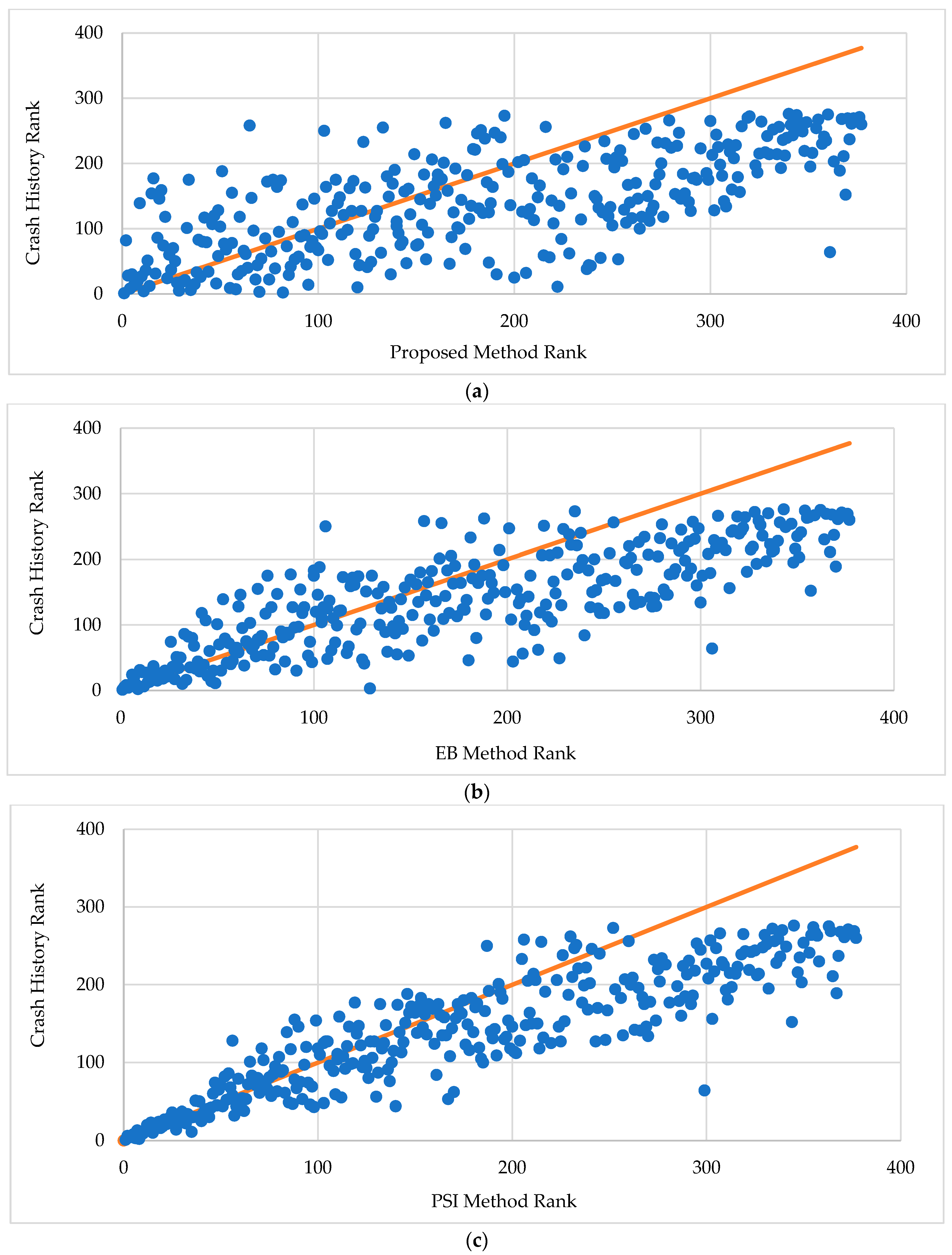
Figure 3 shows a scatterplot with site rankings using the proposed method, EB method, and PSI method versus crash history. An examination of
Figure 3a, which shows the proposed method versus the crash history rank, reveals that the data points are spread around the diagonal line. The discrepancy between the ranks increases with the increase in rank. The tightness of the data points around the line and the correlation coefficient of 0.686 indicates a moderate correlation between the ranks using the two methods. A perfect correlation is a diagonal line passing through the origin.
The EB method ranking was also compared with the ranking using the observed number of crashes and the results are shown in
Figure 3b. In this figure, the proximity of data points to the line passing through the origin (diagonal line) indicates that it is more compact compared to that of the proposed method. This observation is confirmed by a higher correlation coefficient (r = 0.816) between the two rankings.
Additionally,
Figure 3c shows the comparison of ranking using PSI method versus the ranking using the observed number of crashes. The data points clustered around the diagonal line and the correlation coefficient of 0.879 indicate the very strong association between the ranks.
Table 2 presents the Spearman’s rank correlation coefficient values for three different methods (proposed method, Empirical Bayes method, and PSI method) based on crash density and crash frequency in different upper tail segments and for the total sample size of 377 segments. In analyzing the crash density for the upper tail segments (20, 40, 60, 80, 100), the proposed method shows moderate to strong positive correlations with crash history, with values ranging from 0.587 to 0.744. The Empirical Bayes method and PSI method consistently exhibit higher correlations, ranging from 0.786 to 0.828 and 0.954 to 0.959, respectively. For the total sample size of 377 segments, the proposed method exhibits a moderate positive correlation (0.683), while the Empirical Bayes method (0.816) and PSI method (0.879) display stronger positive correlations. This shows that, in analyzing crash densities, the Empirical Bayes and PSI methods outperform the proposed method at identifying safety improvement sites.
In the case of crash frequency, for the upper tail segments (20, 40, 60, 80, 100), the proposed method shows weak to moderate positive correlations, ranging from 0.502 to 0.703. The Empirical Bayes method exhibits overall stronger positive correlations, varying in a broad range from 0.406 to 0.840, while the PSI method consistently demonstrates the highest correlations, ranging from 0.738 to 0.893. In the total sample, the proposed method shows a relatively strong positive correlation (0.815), whereas the Empirical Bayes method (0.928) and PSI method (0.942) display even stronger positive correlations with crash history. This indicates a higher association between all three methods and the crash history when the total sample is analyzed. The difference in performance between the proposed method and the other existing methods can be explained by properly understanding the formulation of the EB and the PSI methods. Specifically, observed crash history is a major contributor to the EB and the PSI methods, which explains the higher correlation between crash history and these methods. On the other hand, observed crash history is not an input to the proposed method.
6.2. True Positive Identification
Secondly, the identification of true positive segments is calculated. A true positive occurs when the proposed method correctly identifies a segment as a potential for safety improvement. This evaluation listed the number and percentage of common segments between two lists: the one compiled using ranks from the proposed method and the other using ranks from observed crash data. The higher the number and percentage of the common sites, the better the performance of the subject method because this indicates a stronger agreement between the prediction of the proposed method and crash history.
Table 3 shows a comparison of the identification of true positive segments by three different methods—the proposed method, the Empirical Bayes (EB) method, and the PSI method—while using observed crash data as a reference in the context of crash density and crash frequency analysis for various upper tail segments.
When evaluating the identification of common segments using crash density, for upper tail segments (20), the proposed method was least consistent with crash history (30%), followed by the EB method (65%) and the PSI method (90%), respectively. With the increase in upper tail segments, the discrepancy between the proposed method and the EB and PSI methods decreases. However, the performance of the proposed method is overall less favorable compared to that of the other two methods. For example, in upper tail segments (100), the proposed method identified 68 sites versus 78 sites for the EB method and 87 sites for the PSI method.
When using crash frequency in the analysis, show better performance for the proposed method and lower discrepancy between the three methods. For instance, the proposed method identified 78% of true positive segments compared to 86% by the EB method and 88% by the PSI method when considering 100 upper tail segments. Further, for every other upper tail considered, the results from the proposed method shows lower discrepancy with those using the other two methods.
6.3. Precision and Percent Deviation
The precision and percent deviation from crash history are calculated for various upper tail segment groups (20, 40, 60, 80, and 100) for the proposed method and the performance is compared with that of the EB and the PSI methods. A higher percentage of precision and lower value of percent deviation indicates better performance.
where
TP, true positive, is the number of sites correctly identified as safety improvement sites by the evaluating method;
FP, false positive, is the number of sites falsely identified as safety improvement sites by the evaluating method (not listed in crash history); and
M is the number of upper tail segments that are considered.
Figure 4 shows precision across various upper tail groups (20, 40, 60, 80, and 100). Precision is also calculated for the EB method, and the PSI method to see how the performance of the proposed method compares to that of the other two methods. The precision percentage based on crash density analysis is shown in
Figure 4a. The figure shows that the precision value is less for the proposed method when compared with the EB and the PSI methods. The value for the proposed method varies from 30% to 68%, versus 62% to 76% for the EB method and 85% to 90% for the PSI methods. On the other hand, the precision percentage based on crash frequency shown in
Figure 4b indicates that the precision value varies from 60% to 78% for the proposed method versus 81.6% to 86% for the EB method and 83.3% to 88% for the PSI method. This confirms that both the EB and PSI methods were more consistent with the crash history compared with the proposed method. Further, the proposed method exhibited better performance and higher consistency with crash history when analyzed using crash frequency over crash density.
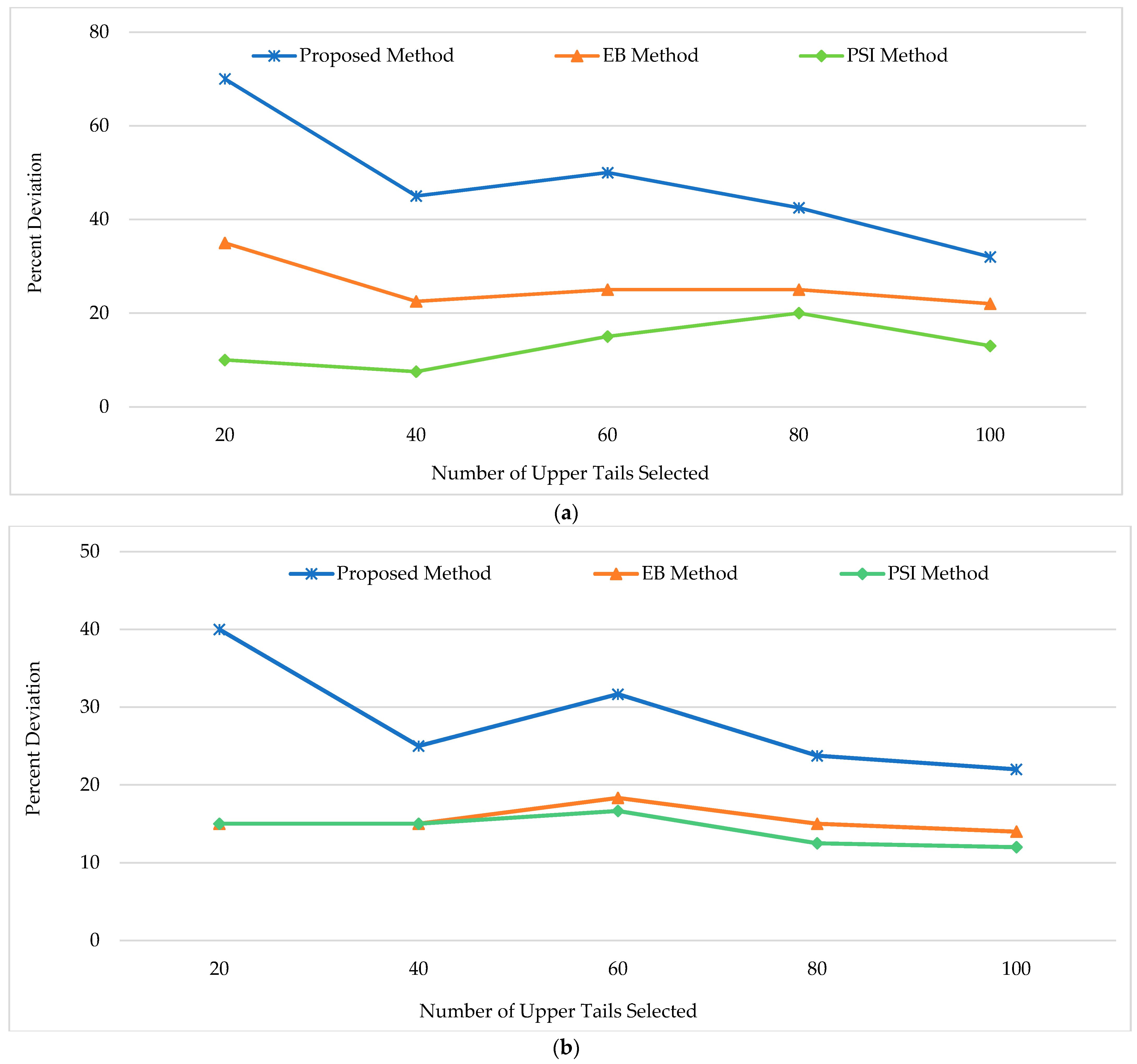
Figure 5 shows the percent deviation from the crash history for the proposed method, the EB method, and the PSI method. A quick examination of
Figure 5 clearly shows higher deviation for the proposed method compared to the EB and the PSI methods both for crash density and crash frequency analyses. The other trend clearly exhibited in this figure is that the percent deviation for the proposed method decreases with the increase in the number of upper tail segments. Specifically, the percent deviation of 70% for density-based analysis and 40% for frequency-based analysis were observed for the 20 upper tail segments. However, the corresponding percent deviation for the 100 upper tails is 32% and 22% for density-based and frequency-based analyses, respectively. The EB and the PSI methods, while generally showing less deviation and better performance, exhibited less variation in percent deviation with the increase in upper tail segments.
6.4. Treatable Crashes
The last analysis in the evaluation of the proposed method involved the use of the number of treatable crashes (calculated for five years: 2016–2020) as the performance measure. Treatable crashes are defined as those crashes that may be treated by engineering countermeasures such as lane widening. The remaining crashes constitute what might be expected due to traffic exposure and may not be treatable by engineering countermeasures. A reasonable estimate for the number of treatable crashes at a location is the number of crashes in excess of what would normally be expected at locations with similar characteristics and traffic exposure [
29]. To assess the degree of similarity between the segments identified by a method and those identified by the crash history, a segment overlap metric was used. The higher the percentage of segment overlap and the closer the estimate of treatable crashes with crash history, the better the performance of the compared method.
Table 4 shows the summary of the estimate of treatable crashes for the proposed method the EB method, and crash history. The table also provides the ratio and overlap for treatable crashes in the top 100 segments defined earlier using both crash density and crash frequency.
The table shows that, based on crash density, the proposed method identified a fewer number of treatable crashes for the top 100 segments compared to crash history (469 versus 726, respectively). The segment overlap was 66%. Using crash frequency, the segment overlap increased to 79% indicating a significant improvement in performance. Regarding the EB method, the number of treatable crashes and overlap indicate a higher level of consistency with crash history. However, the discrepancy in performance between the proposed and the EB methods is less evident when crash frequency is used in the analysis. Specifically, there were only 11.6% fewer treatable crashes on the segments identified with the proposed method than those identified with the crash history, compared to 11.3% fewer treatable crashes using the EB method. Further, 79% of all segments identified by the proposed method were also on the top 100 segments list of the observed crash.
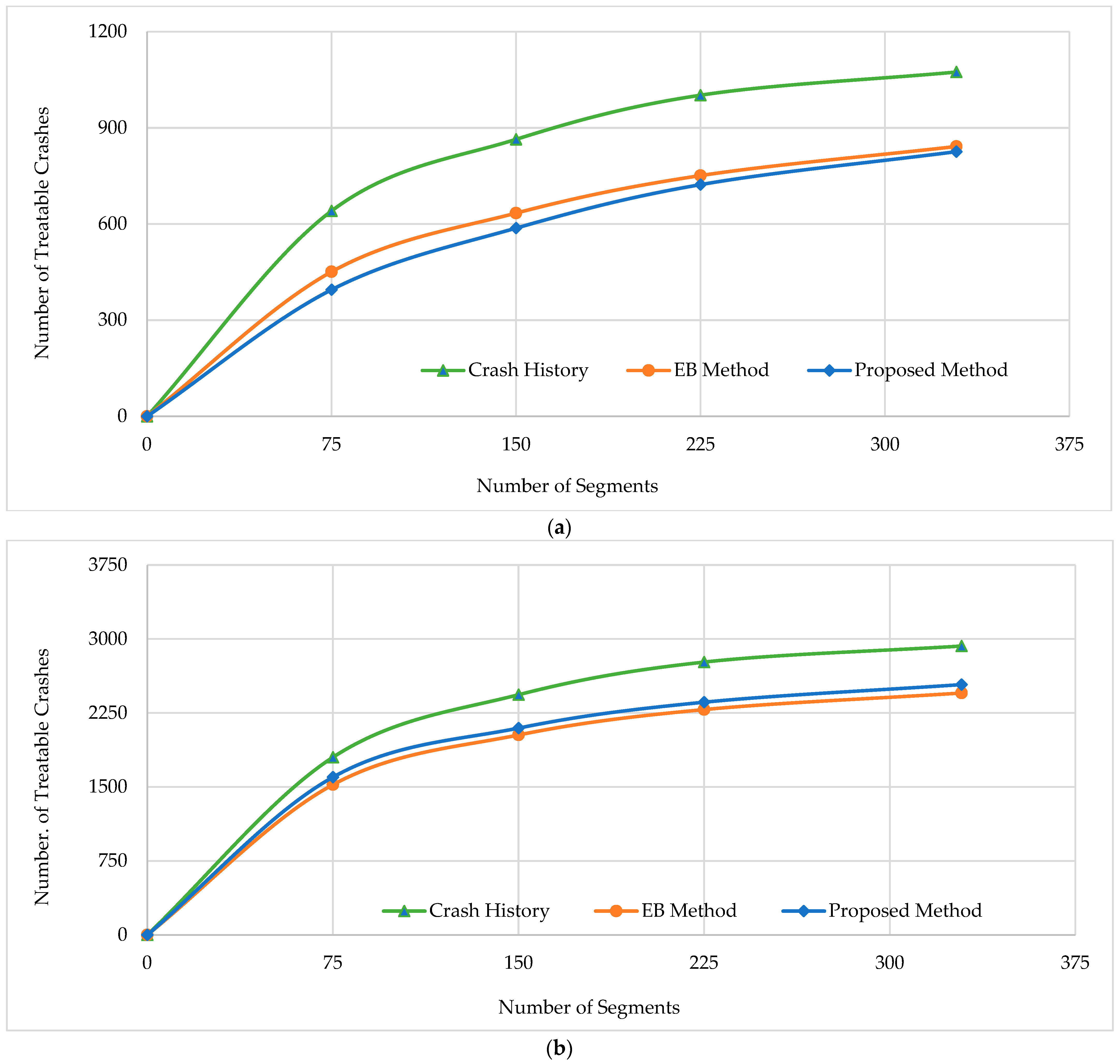
In addition to evaluating the top 100 segments identified by the methods, similar calculations were performed for other possible levels of selection up to upper tails having positive treatable crashes. Plots of the treatable crashes identified at various levels are shown in
Figure 6. For the range of top segments studied, the chart shows relatively close lines for the proposed and the EB methods, with the EB method consistently identifying a slightly higher number of treatable crashes. The figure also suggests that the larger the total segments selected, the closer the proposed method is in terms of selection efficiency compared to that of EB method. These patterns are similar for the crash density and crash frequency analyses.
7. Summary and Conclusions
Network screening is a critical initial step of the highway safety improvement programs which aims to identify sites with potential for safety improvement. Ineffective network screening can lead to a significant number of false positives and/or false negatives resulting in an inefficient allocation of agency resources and consequently impacting the overall efficacy of safety management programs. Hence, the accurate identification of sites that are in need of safety improvements is crucial for the success of any highway safety program.
The research presented in this paper examined a new proposed approach for identifying safety improvement sites on rural highways. The proposed approach involves the use of EB prediction models using traffic and roadway variables only. Specifically, the multiple linear regression was used to develop a mathematical model to predict the EB expected number of crashes. The proposed model utilizes classified variables for roadway and roadside characteristics that do not require detailed databases or extensive technical expertise. The evaluation was performed using a dataset comprising 1495 miles of rural two-lane highway segments in the state of Oregon. The data used in the evaluation included roadway geometry, roadside features, traffic conditions, and ten years of crash records. A training dataset spanning five years (2011–2015) was employed to develop the model, while the subsequent five-year period (2016–2020) served as the basis for evaluating the model’s performance in network screening.
The study findings suggest that using crash density for highway segments, the performance of the proposed method was fair and not as effective as the well-established EB and PSI methods. This is despite the high R-square value of the predictive model used by the proposed approach. However, when using crash frequencies for highway segments, the performance of the proposed method was found to be comparable to the EB and PSI methods. Moreover, the results suggest that, in identifying segments most likely to have treatable crashes, the proposed method outperformed the EB method for higher upper tail segments considered in the analysis. Despite the overall lower performance of the proposed method, it provides a valuable tool to local agencies where the application of the more sophisticated methods is deemed impractical for lack of resources.
To promote the use of the proposed method in practice, further evaluation using highway networks from other regions and states may reinforce the evidence about the effectiveness of the proposed method in identifying safety improvement sites. Further, evaluating the proposed approach at rural highway intersections would make the use of the proposed method more attractive to local agencies by applying the same approach to various highway network components (i.e., segments and intersections).
Author Contributions
The authors confirm contribution to the paper as follows: study conception and design: A.A.-K.; data collection: B.D.; analysis and interpretation of results: B.D. and A.A.-K.; draft manuscript preparation: B.D. and A.A.-K. All authors have read and agreed to the published version of the manuscript.
Funding
This work was supported by the US Department of Transportation (USDOT) Small Urban, Rural, and Tribal Center on Mobility (SURTCOM) at the Western Transportation Institute of Montana State University.
Institutional Review Board Statement
Not applicable.
Informed Consent Statement
Not applicable.
Data Availability Statement
The data presented in this study are available on request from the corresponding author. The data are not publicly available due to privacy.
Conflicts of Interest
The authors declare no conflicts of interest.
References
- Fatality Facts 2021: Urban/Rural Comparison. Available online: https://www.iihs.org/topics/fatality-statistics/detail/urban-rural-comparison (accessed on 20 July 2023).
- Schmelkin, E.J.P.; Pedhazur, L. Measurement, Design, and Analysis: An Integrated Approach; Psychology Press: New York, NY, USA, 1991; ISBN 978-0-203-72638-9. [Google Scholar]
- Hauer, E.; Kononov, J.; Allery, B.; Griffith, M.S. Screening the Road Network for Sites with Promise. Transp. Res. Rec. 2002, 1784, 27–32. [Google Scholar] [CrossRef]
- Park, P.Y.; Sahaji, R. Safety Network Screening for Municipalities with Incomplete Traffic Volume Data. Accid. Anal. Prev. 2013, 50, 1062–1072. [Google Scholar] [CrossRef]
- Anastasopoulos, P.C.; Mannering, F.L. An Empirical Assessment of Fixed and Random Parameter Logit Models Using Crash- and Non-Crash-Specific Injury Data. Accid. Anal. Prev. 2011, 43, 1140–1147. [Google Scholar] [CrossRef]
- Agerholm, N.; Lahrmann, H. Identification of Hazardous Road Locations on the Basis of Floating Car Data: Method and First Results. In Road Safety in a Globalised and More Sustainable World-Current Issues and Future Challenges; International Co-Operation on Theories and Concepts in Traffic Safety (ICTCT): Hasselt, Belgium, 2012. [Google Scholar]
- Huang, H.; Chin, H.C.; Haque, M.d.M. Empirical Evaluation of Alternative Approaches in Identifying Crash Hot Spots: Naive Ranking, Empirical Bayes, Full Bayes Methods. Transp. Res. Rec. 2009, 2103, 32–41. [Google Scholar] [CrossRef]
- Lee, C.; Hellinga, B.; Ozbay, K. Quantifying Effects of Ramp Metering on Freeway Safety. Accid. Anal. Prev. 2006, 38, 279–288. [Google Scholar] [CrossRef]
- Huda, K.T. Developing a Network Screening Method for Low Volume Roads. Master’s Thesis, Montana State University, College of Engineering, Bozeman, MT, USA, 2020. [Google Scholar]
- Cheng, W.; Washington, S.P. Experimental Evaluation of Hotspot Identification Methods. Accid. Anal. Prev. 2005, 37, 870–881. [Google Scholar] [CrossRef] [PubMed]
- Kwon, O.H.; Park, M.J.; Yeo, H.; Chung, K. Evaluating the Performance of Network Screening Methods for Detecting High Collision Concentration Locations on Highways. Accid. Anal. Prev. 2013, 51, 141–149. [Google Scholar] [CrossRef] [PubMed]
- Ambros, J.; Valentová, V.; Janoška, Z. Investigation of Difference between Network Screening Results Based on Multivariate and Simple Crash Prediction Models. In Proceedings of the 94th Annual Meeting of the Transportation Research Board, Washington, DC, USA, 13 January 2015. [Google Scholar]
- Mesquita Xavier, V.J.; Craveiro Cunto, F.J. Comparative Analysis of Performance Measures for Network Screening: A Case Study of Brazilian Urban Areas. J. Adv. Transp. 2017, 2017, e4360414. [Google Scholar] [CrossRef]
- Montella, A. A Comparative Analysis of Hotspot Identification Methods. Accid. Anal. Prev. 2010, 42, 571–581. [Google Scholar] [CrossRef] [PubMed]
- Gross, F.B.; Harmon, T.; Albee, M.; Himes, S.; Srinivasan, R.; Carter, D.; Dugas, M. Evaluation of Four Network Screening Performance Measures; Federal Highway Administration, Office of Safety: Washington, DC, USA, 2016.
- Elvik, R. State-of-the-Art Approaches to Road Accident Black Spot Management and Safety Analysis of Road Networks; Transportøkonomisk institutt: Oslo, Norway, 2007. [Google Scholar]
- Cheng, W.; Washington, S. New Criteria for Evaluating Methods of Identifying Hot Spots. Transp. Res. Rec. 2008, 2083, 76–85. [Google Scholar] [CrossRef]
- ODOT TransGIS. Available online: https://gis.odot.state.or.us/transgis (accessed on 6 June 2023).
- Oregon Department of Transportation: Road Assets and Mileage: Data & Maps: State of Oregon. Available online: https://www.oregon.gov/odot/Data/pages/road-assets-mileage.aspx (accessed on 6 June 2023).
- TDS—Crash Reports. Available online: https://tvc.odot.state.or.us/tvc/ (accessed on 6 June 2023).
- Cafiso, S.; Di Silvestro, G.; Persaud, B.; Begum, M.A. Revisiting Variability of Dispersion Parameter of Safety Performance for Two-Lane Rural Roads. Transp. Res. Rec. 2010, 2148, 38–46. [Google Scholar] [CrossRef]
- Manepalli, U.R.R.; Bham, G.H. An Evaluation of Performance Measures for Hotspot Identification. J. Transp. Saf. Secur. 2016, 8, 327–345. [Google Scholar] [CrossRef]
- Manepalli, U.R.R.; Bham, G.H. Crash Prediction: Evaluation of Empirical Bayes AND Kriging methods. In Proceedings of the 3rd International Conference on Road Safety and Simulation, Indianapolis, IN, USA, 14–16 September 2011. [Google Scholar]
- Elvik, R. The Predictive Validity of Empirical Bayes Estimates of Road Safety. Accid. Anal. Prev. 2008, 40, 1964–1969. [Google Scholar] [CrossRef] [PubMed]
- Hauer, E. Observational Before–after Studies in Road Safety: Estimating the Effect of Highway and Traffic Engineering Measures on Road Safety; Pergamon: Amsterdam, The Netherlands, 2002; ISBN 978-0-08-043053-9. [Google Scholar]
- Persaud, B.; Lyon, C. Empirical Bayes before-after Safety Studies: Lessons Learned from Two Decades of Experience and Future Directions. Accid. Anal. Prev. 2007, 39, 546–555. [Google Scholar] [CrossRef] [PubMed]
- Hauer, E.; Persaud, B.N.; Smiley, A.; Duncan, D. Estimating the Accident Potential of an Ontario Driver. Accid. Anal. Prev. 1991, 23, 133–152. [Google Scholar] [CrossRef] [PubMed]
- Hauke, J.; Kossowski, T. Comparison of Values of Pearson’s and Spearman’s Correlation Coefficients on the Same Sets of Data. QUAGEO 2011, 30, 87–93. [Google Scholar] [CrossRef]
- Persaud, B.; Lyon, C.; Nguyen, T. Empirical Bayes Procedure for Ranking Sites for Safety Investigation by Potential for Safety Improvement. Transp. Res. Rec. 1999, 1665, 7–12. [Google Scholar] [CrossRef]
| Disclaimer/Publisher’s Note: The statements, opinions and data contained in all publications are solely those of the individual author(s) and contributor(s) and not of MDPI and/or the editor(s). MDPI and/or the editor(s) disclaim responsibility for any injury to people or property resulting from any ideas, methods, instructions or products referred to in the content. |
© 2024 by the authors. Licensee MDPI, Basel, Switzerland. This article is an open access article distributed under the terms and conditions of the Creative Commons Attribution (CC BY) license (https://creativecommons.org/licenses/by/4.0/).


