

A Novel Approach to Swell Mitigation: Machine-Learning-Powered Optimal Unit Weight and Stress Prediction in Expansive Soils


Abstract
1. Introduction
- (1)
- Collecting information on the damage that has occurred in the study area, the risk reduction methods employed, and their effectiveness.
- (2)
- Conducting a comprehensive analysis of the soil and its properties (in situ and laboratory testing) by a geotechnical engineering expert.
- (3)
- Classifying the degree of severity of the expansive soil based on the findings from steps 1 and 2.
- (4)
- Proposing an appropriate risk mitigation strategy.
- Place a high permeability soil layer beneath the entire building with sufficient thickness to ensure uniform moisture conditions under the structure [25].
- Use a machine learning model to determine the optimal dry unit weight for expansive soil as a fill material, or the optimal stress to achieve the lowest volumetric change.
- Design a suitable foundation that can deliver the required stress based on the building’s specifications.
- Isolate any external factors that could influence soil moisture content, such as nearby trees, to prevent tree roots from absorbing moisture from beneath the structure [24].
2. Materials and Methods
2.1. Materials and Classification Tests
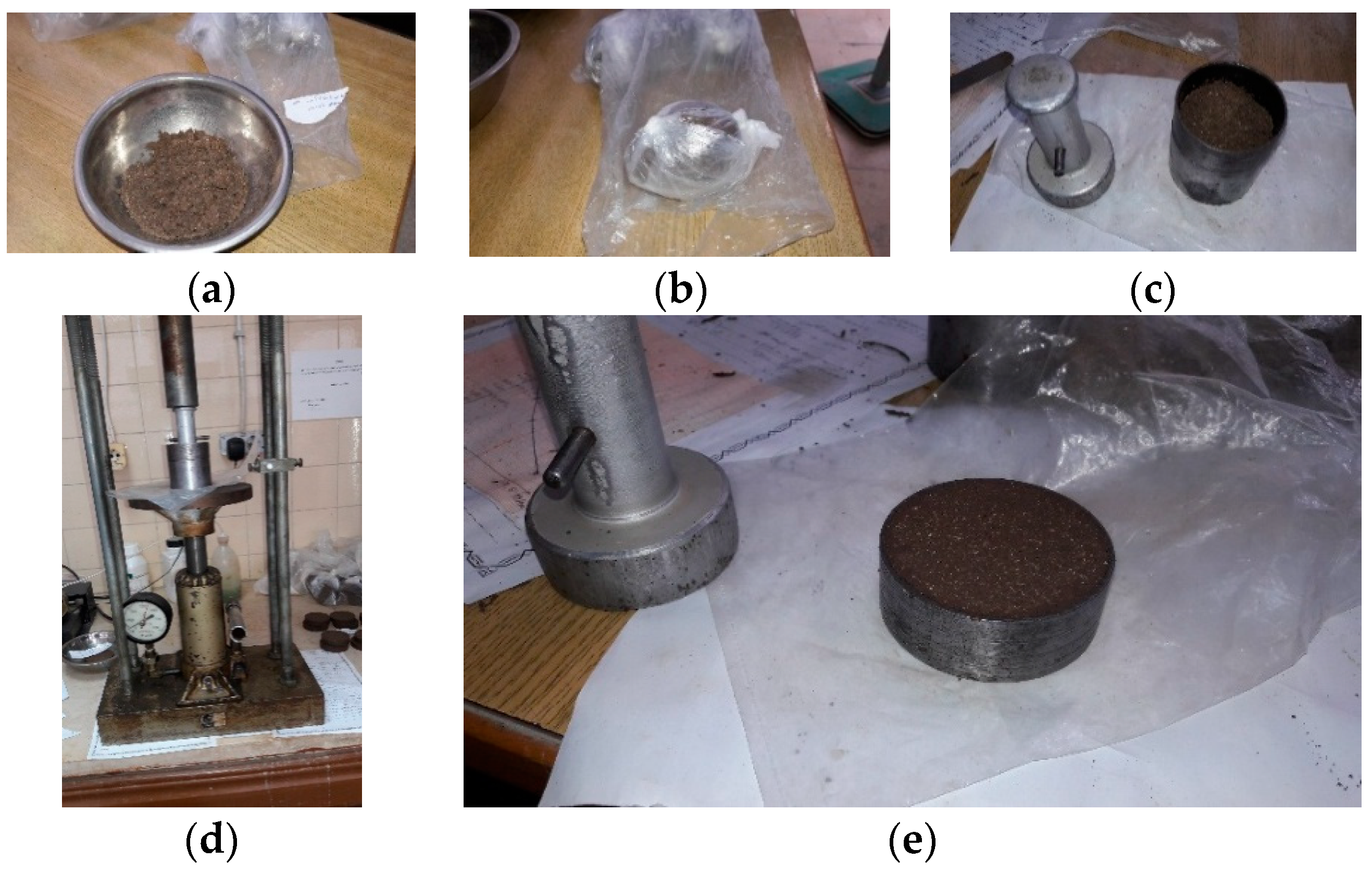
2.2. Samples Preparation
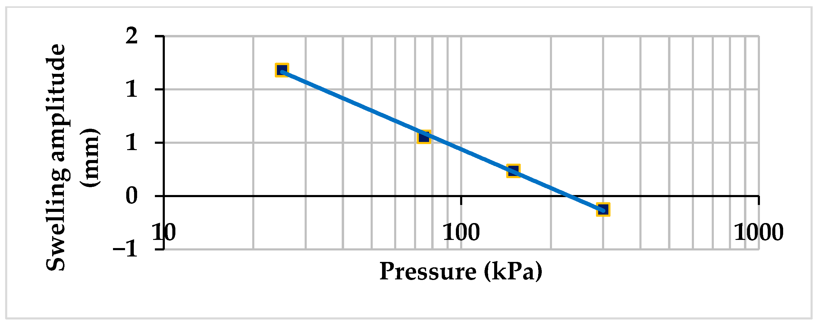
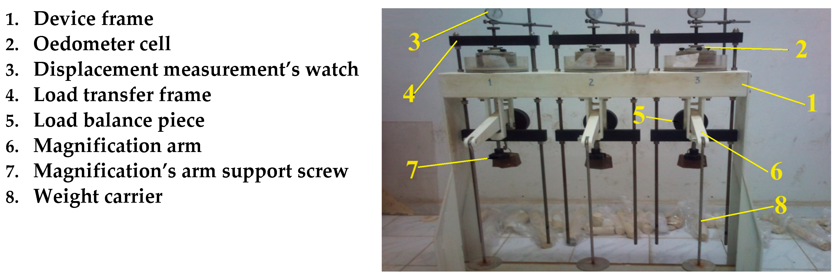
2.3. Loaded Swelling Pressure Tests
2.4. Selection of Variables
2.5. Machine Learning Algorithms Used in the Study
2.5.1. Decision Tree Regression
2.5.2. Random Forest Regression
2.5.3. Gradient Boosting Regression
2.5.4. Extreme Gradient Boosting
2.5.5. Support Vector Regression
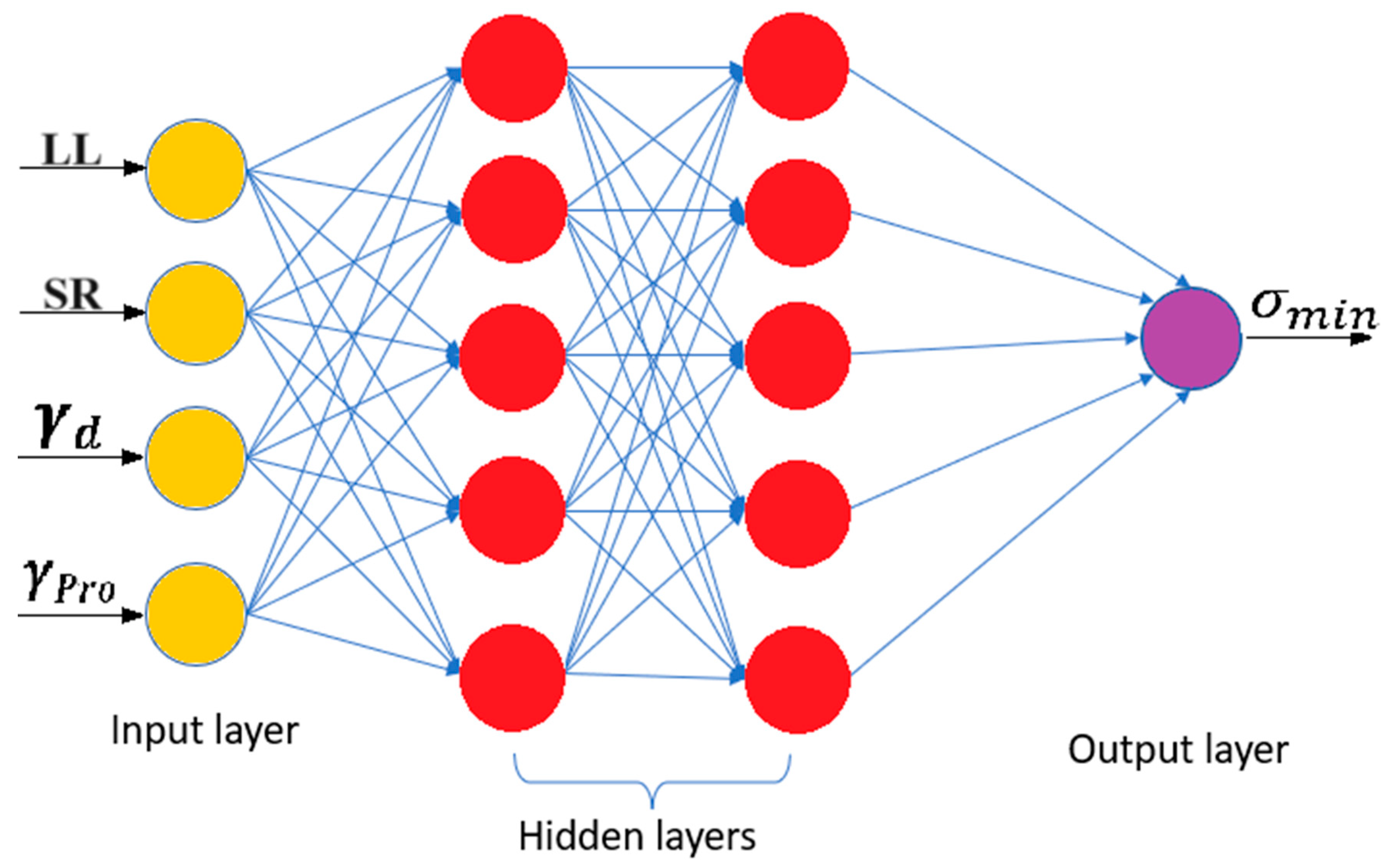
2.5.6. Artificial Neural Networks
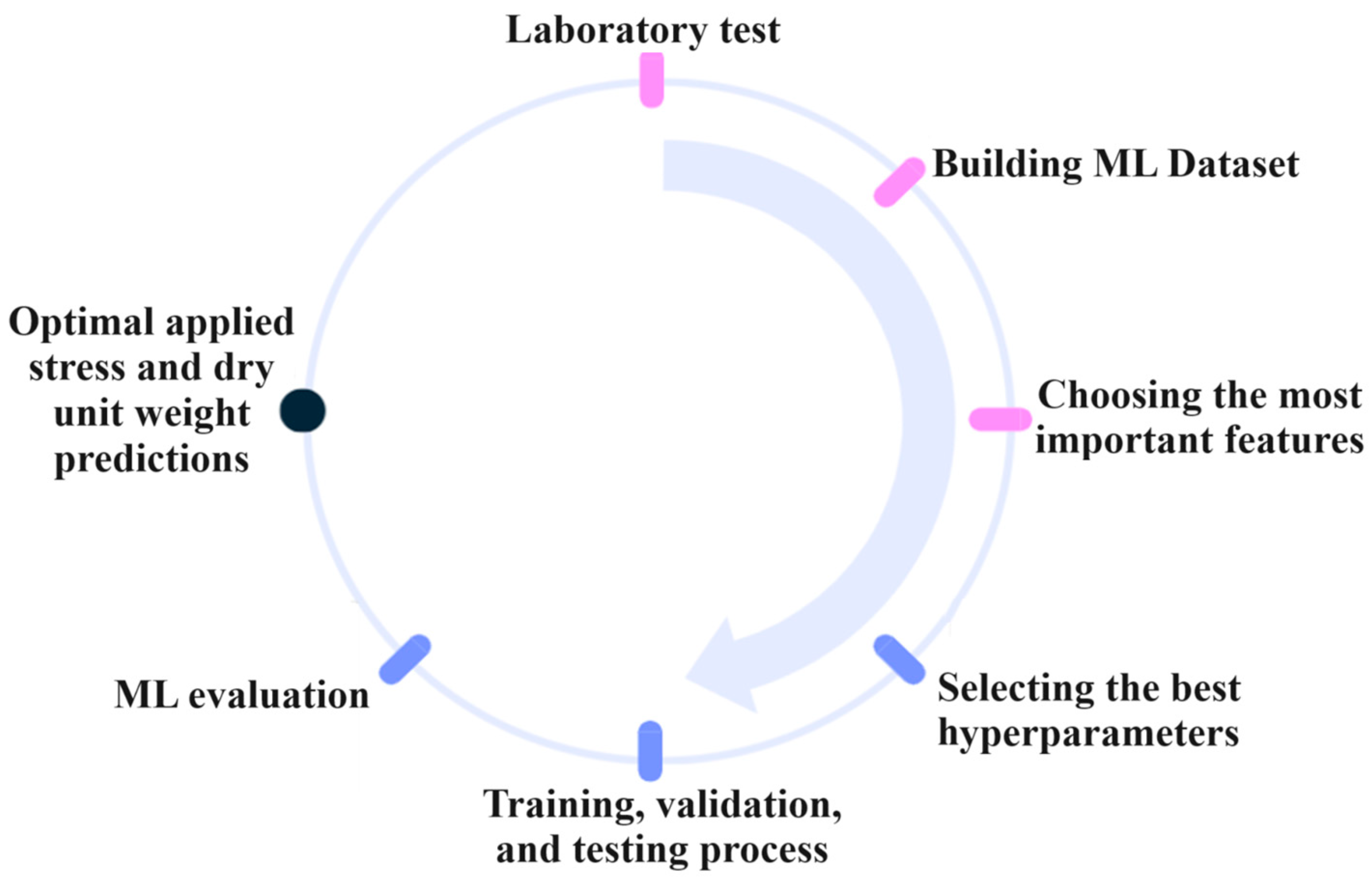
2.6. Building the Dataset and Evaluation of the Models
- Y, Yj—refers to the observed values and expected values by machine learning models.
- , —are the average of Y, Yj, respectively.
- N—represents the number of data.
2.7. Hyperparameters Optimization
3. Results and Discussion
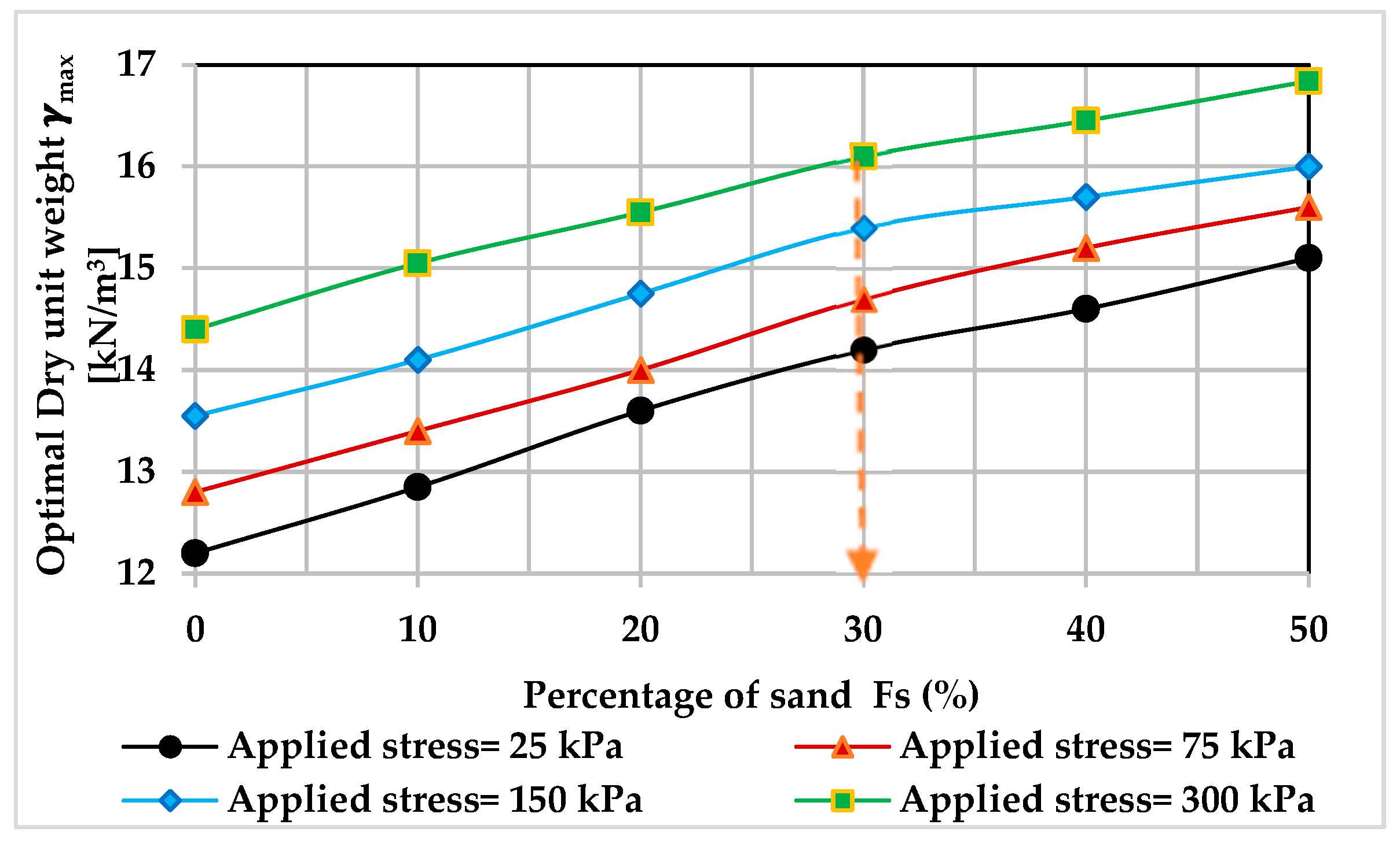
3.1. Experimental Work Results and Discussion
3.2. Machine Learning Results and Discussion
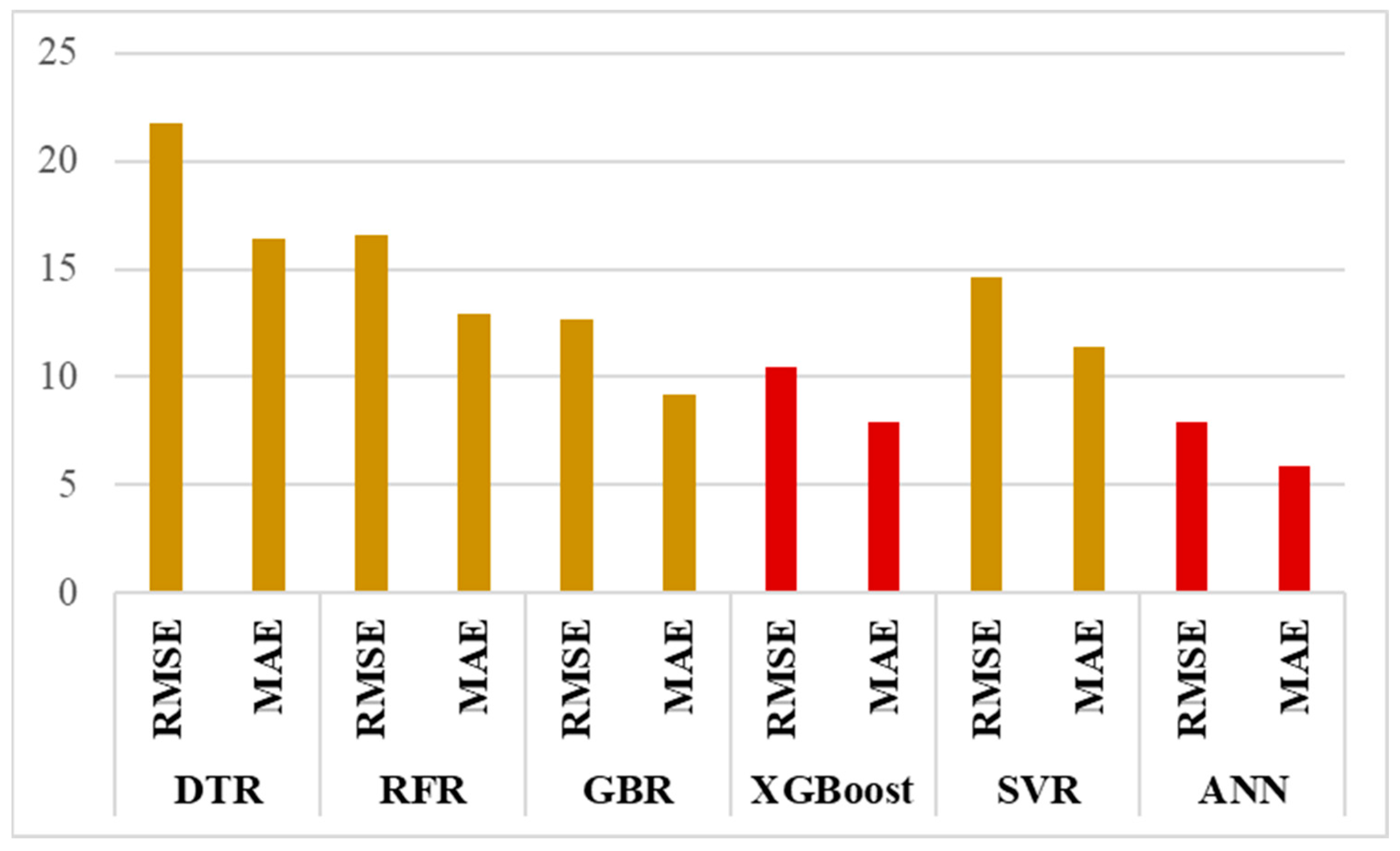
3.2.1. Comparison of Machine Learning Models
3.2.2. Models Results
DTR Model Results
RFR Model Result
GBR Model Results
XGBoost Model Results
SVR Model Results
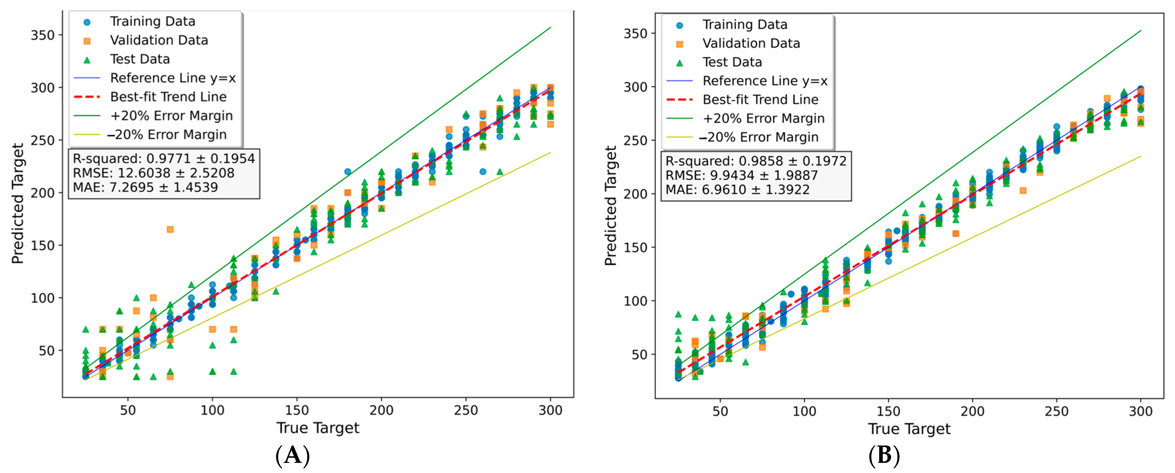
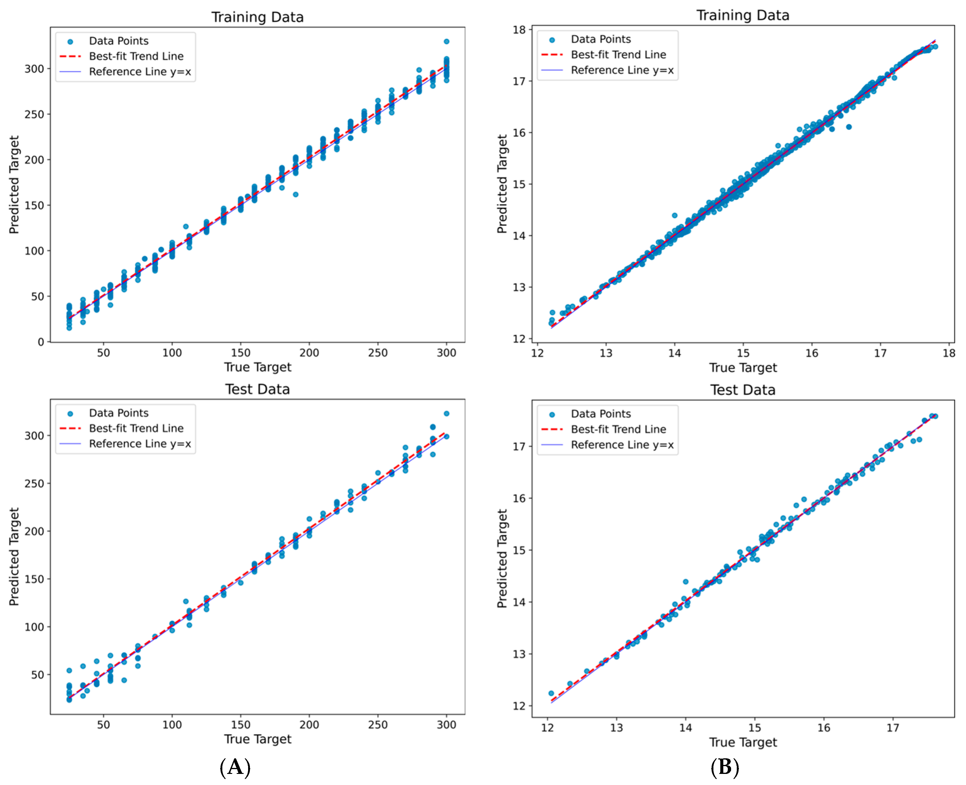
ANN Model Results
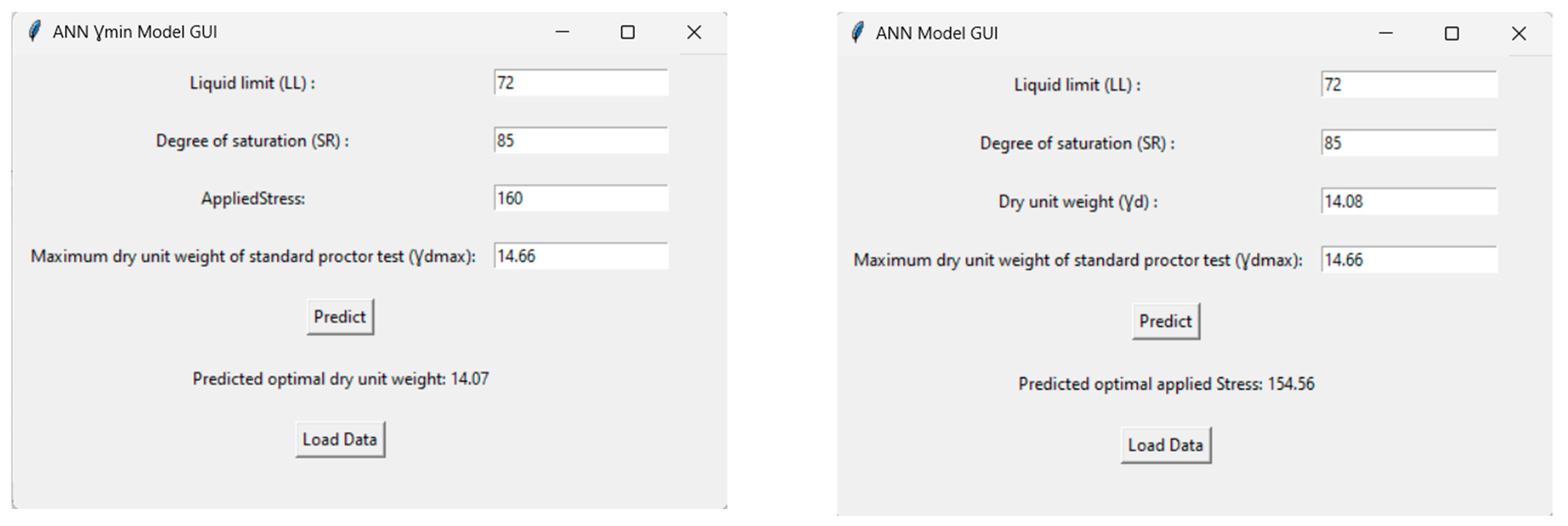
3.2.3. Streamlined Interface for ANN Model Predictions
4. Conclusions
Supplementary Materials
Author Contributions
Funding
Institutional Review Board Statement
Informed Consent Statement
Data Availability Statement
Conflicts of Interest
References
- Stoll, S.C.; Henning, S.R.; Bagley, A.D.; Wieghaus, K.T. Foundation Damage Assessments and Structural Repairs. In Forensic Engineering; American Society of Civil Engineers: Denver, CO, USA, 2022; pp. 166–174. ISBN 9780784484548. [Google Scholar]
- Fredlund, D.G.; Rahardjo, H. Soil Mechanics for Unsaturated Soils; John Wiley & Sons, Inc.: Hoboken, NJ, USA, 1993; ISBN 9780470172759. [Google Scholar]
- Mokhtari, M.; Dehghani, M. Swell-Shrink Behavior of Expansive Soils, Damage and Control. Electron. J. Geotech. Eng. 2012, 17, 2673–2682. [Google Scholar]
- Federal Highway Administration. Chapter 4: Soil and Rock Behavior. In A Quarter Century of Geotechnical Research; FHWA-RD-98-139; Federal Highway Administration: Washinton, DC, USA, 1999. [Google Scholar]
- Sawangsuriya, A.; Jotisankasa, A.; Anuvechsirikiat, S. Classification of Shrinkage and Swelling Potential of a Subgrade Soil in Central Thailand. In Unsaturated Soils: Research and Applications; Springer: Berlin/Heidelberg, Germany, 2012; pp. 325–331. [Google Scholar]
- Márta, F. Development of the Classification of High Swelling Clay Content Soils of Hungary Based on Diagnostic Approach. Ph.D. Thesis, Szent István University, Gödöllő, Hungary, 2012. [Google Scholar]
- Teodosio, B.; Kristombu Baduge, K.S.; Mendis, P. A Review and Comparison of Design Methods for Raft Substructures on Expansive Soils. J. Build. Eng. 2021, 41, 102737. [Google Scholar] [CrossRef]
- Ijaz, N.; Ye, W.; ur Rehman, Z.; Dai, F.; Ijaz, Z. Numerical Study on Stability of Lignosulphonate-Based Stabilized Surficial Layer of Unsaturated Expansive Soil Slope Considering Hydro-Mechanical Effect. Transp. Geotech. 2022, 32, 100697. [Google Scholar] [CrossRef]
- Steinberg, M.L. Controlling Expansive Soil Destructiveness by Deep Vertical Geomembranes on Four Highways; Transportation Research Board: Washinton, DC, USA, 1985; ISBN 0309039231. [Google Scholar]
- Goodarzi, A.R.; Akbari, H.R.; Salimi, M. Enhanced Stabilization of Highly Expansive Clays by Mixing Cement and Silica Fume. Appl. Clay Sci. 2016, 132–133, 675–684. [Google Scholar] [CrossRef]
- Kolay, P.K.; Ramesh, K.C. Reduction of Expansive Index, Swelling and Compression Behavior of Kaolinite and Bentonite Clay with Sand and Class C Fly Ash. Geotech. Geol. Eng. 2016, 34, 87–101. [Google Scholar] [CrossRef]
- Salimi, M.; Ilkhani, M.; Vakili, A.H. Stabilization Treatment of Na-Montmorillonite with Binary Mixtures of Lime and Steelmaking Slag. Int. J. Geotech. Eng. 2020, 14, 295–301. [Google Scholar] [CrossRef]
- Nelson, J.; Miller, D.J. Expansive Soils: Problems and Practice in Foundation and Pavement Engineering; John Wiley & Sons: Hoboken, NJ, USA, 1997. [Google Scholar]
- Roy, T.K. Influence of Sand on Strength Characteristics of Cohesive Soil for Using as Subgrade of Road. Procedia-Soc. Behav. Sci. 2013, 104, 218–224. [Google Scholar] [CrossRef]
- Mohamed, K.; Abdelkrim, M.; Lakhdar, M. Problematic Soil Mechanics in the Algerian Arid and Semi-Arid Regions: Case of M’sila Expansive Clays. J. Appl. Eng. Sci. Technol. 2015, 1, 37–41. [Google Scholar]
- Al Rawi, O.S.; Assaf, M.N.; Hussein, N.M. Effect of Sand Additives on the Engineering Properties of Fine Grained Soils. ARPN J. Eng. Appl. Sci. 2018, 13, 3197–3206. [Google Scholar]
- Phanikumar, B.R.; Dembla, S.; Yatindra, A. Swelling Behaviour of an Expansive Clay Blended with Fine Sand and Fly Ash. Geotech. Geol. Eng. 2021, 39, 583–591. [Google Scholar] [CrossRef]
- Alnmr, A.; Ray, R.P. Review of the Effect of Sand on the Behavior of Expansive Clayey Soils. Acta Tech. Jaurinensis 2021, 14, 521–552. [Google Scholar] [CrossRef]
- Lamara, M.; Gueddouda, M.K.; Benabed, B. Stabilisation Physico-Chimique Des Sols Gonflants (Sable de Dune + Sel). Rev. Française Géotechn. 2006, 115, 25–35. [Google Scholar] [CrossRef][Green Version]
- Prasad, C.R.V.; Sharma, R.K. Influence of Sand and Fly Ash on Clayey Soil Stabilization. IOSR J. Mech. Civ. Eng. 2014, 334, 36–40. [Google Scholar]
- Nagaraj, H.B. Influence of Gradation and Proportion of Sand on Stress–Strain Behavior of Clay–Sand Mixtures. Int. J. Geo-Eng. 2016, 7, 19. [Google Scholar] [CrossRef]
- Srikanth, V.; Mishra, A.K. Atterberg Limits of Sand-Bentonite Mixes and the Influence of Sand Composition. In Geotechnical Characterisation and Geoenvironmental Engineering; Springer: Berlin/Heidelberg, Germany, 2019; pp. 139–145. [Google Scholar] [CrossRef]
- Dasog, G.S.; Mermut, A.R. Expansive Soils and Clays. Encycl. Earth Sci. Ser. 2013, 297–300. [Google Scholar] [CrossRef]
- Jones, L.D.; Jefferson, I. Expansive Soils. In ICE Manual of Geotechnical Engineering. Volume 1: Geotechnical Engineering Principles, Problematic Soils and Site Investigation; Burland, J., Ed.; ICE Manual of Geotechnical Engineering: London, UK, 2012. [Google Scholar]
- Alnmr, A.; Ray, R. Numerical Simulation of Replacement Method to Improve Unsaturated Expansive Soil. Pollack Period. 2023, 18, 41–47. [Google Scholar] [CrossRef]
- Dawson, R.F.; Altmeyer, W.T.; Barber, E.S.; DuBose, L.A. Discussion of “Engineering Properties of Expansive Clays”. Trans. Am. Soc. Civ. Eng. 1956, 121, 664–675. [Google Scholar] [CrossRef]
- Seed, H.B.; Woodward, R.J.; Lundgren, R. Prediction of Swelling Potential for Compacted Clays. Trans. Am. Soc. Civ. Eng. 1963, 128, 1443–1477. [Google Scholar] [CrossRef]
- Ranganatham, B.V.; Satyanarayana, B. A Rational Method of Predicting Swelling Potential for Compacted Expansive Clays. In Proceedings of the 6th International Conference on Soil Mechanics and Foundation Engineering, Montréal, QC, Canada, 8–15 September 1965; pp. 92–96. [Google Scholar]
- Snethen, D.R. Evaluation of Expedient Methods for Identification and Classification of Potentially Expansive Soils. In Proceedings of the Fifth International Conference on Expansive Soils 1984, Adelaide, Australia, 21–23 May 1984; pp. 22–26. [Google Scholar]
- Al-Shayea, N.A. The Combined Effect of Clay and Moisture Content on the Behavior of Remolded Unsaturated Soils. Eng. Geol. 2001, 62, 319–342. [Google Scholar] [CrossRef]
- Yilmaz, I. Indirect Estimation of the Swelling Percent and a New Classification of Soils Depending on Liquid Limit and Cation Exchange Capacity. Eng. Geol. 2006, 85, 295–301. [Google Scholar] [CrossRef]
- Çimen, Ö.; Keskin, S.N.; Yıldırım, H. Prediction of Swelling Potential and Pressure in Compacted Clay. Arab. J. Sci. Eng. 2012, 37, 1535–1546. [Google Scholar] [CrossRef]
- Ling, Q.; Zhang, Q.; Wei, Y.; Kong, L.; Zhu, L. Slope Reliability Evaluation Based on Multi-Objective Grey Wolf Optimization-Multi-Kernel-Based Extreme Learning Machine Agent Model. Bull. Eng. Geol. Environ. 2021, 80, 2011–2024. [Google Scholar] [CrossRef]
- Liu, L.; Zhang, S.; Cheng, Y.M.; Liang, L. Advanced Reliability Analysis of Slopes in Spatially Variable Soils Using Multivariate Adaptive Regression Splines. Geosci. Front. 2019, 10, 671–682. [Google Scholar] [CrossRef]
- Wang, H.; Zhang, L.; Yin, K.; Luo, H.; Li, J. Landslide Identification Using Machine Learning. Geosci. Front. 2021, 12, 351–364. [Google Scholar] [CrossRef]
- Ray, R.; Kumar, D.; Samui, P.; Roy, L.B.; Goh, A.T.C.; Zhang, W. Application of Soft Computing Techniques for Shallow Foundation Reliability in Geotechnical Engineering. Geosci. Front. 2021, 12, 375–383. [Google Scholar] [CrossRef]
- Wang, L.; Wu, C.; Tang, L.; Zhang, W.; Lacasse, S.; Liu, H.; Gao, L. Efficient Reliability Analysis of Earth Dam Slope Stability Using Extreme Gradient Boosting Method. Acta Geotech. 2020, 15, 3135–3150. [Google Scholar] [CrossRef]
- Merouane, F.Z.; Mamoune, S.M.A. Prediction of Swelling Parameters of Two Clayey Soils from Algeria Using Artificial Neural Networks. Math. Model. Civ. Eng. 2018, 14, 11–26. [Google Scholar] [CrossRef]
- Dutta, R.K.; Singh, A.; Gnananandarao, T. Prediction of Free Swell Index for the Expansive Soil Using Artificial Neural Networks. J. Soft Comput. Civ. Eng. 2019, 3, 47–62. [Google Scholar] [CrossRef]
- Cho, S.E. Probabilistic Stability Analyses of Slopes Using the ANN-Based Response Surface. Comput. Geotech. 2009, 36, 787–797. [Google Scholar] [CrossRef]
- Li, S.; Zhao, H.B.; Ru, Z. Slope Reliability Analysis by Updated Support Vector Machine and Monte Carlo Simulation. Nat. Hazards 2013, 65, 707–722. [Google Scholar] [CrossRef]
- Li, T.Z.; Pan, Q.; Dias, D. Active Learning Relevant Vector Machine for Reliability Analysis. Appl. Math. Model. 2021, 89, 381–399. [Google Scholar] [CrossRef]
- Kardani, N.; Aminpour, M.; Nouman Amjad Raja, M.; Kumar, G.; Bardhan, A.; Nazem, M. Prediction of the Resilient Modulus of Compacted Subgrade Soils Using Ensemble Machine Learning Methods. Transp. Geotech. 2022, 36, 100827. [Google Scholar] [CrossRef]
- Yi, P.; Wei, K.; Kong, X.; Zhu, Z. Cumulative PSO-Kriging Model for Slope Reliability Analysis. Probabilistic Eng. Mech. 2015, 39, 39–45. [Google Scholar] [CrossRef]
- Kumar, M.; Samui, P. Reliability Analysis of Pile Foundation Using ELM and MARS. Geotech. Geol. Eng. 2019, 37, 3447–3457. [Google Scholar] [CrossRef]
- Shen, H.; Li, J.; Wang, S.; Xie, Z. Prediction of Load-Displacement Performance of Grouted Anchors in Weathered Granites Using FastICA-MARS as a Novel Model. Geosci. Front. 2021, 12, 415–423. [Google Scholar] [CrossRef]
- Zhang, W.; Wu, C.; Tang, L.; Gu, X.; Wang, L. Efficient Time-Variant Reliability Analysis of Bazimen Landslide in the Three Gorges Reservoir Area Using XGBoost and LightGBM Algorithms. Gondwana Res. 2022, 123, 41–53. [Google Scholar] [CrossRef]
- Najjar, Y.M.; Basheer, I.A.; Mcreynolds, R. Neural Modeling of Kansas Soil Swelling. Transp. Res. Rec. J. Transp. Res. Board. 1996, 1526, 14–19. [Google Scholar] [CrossRef]
- Najjar, Y.M.; Basheer, I.A. Modeling of Soil Swelling via Regression and Neural Network Approaches; Kansas Department of Transportation: Topeka, KS, USA, 1998. [Google Scholar]
- Doris, J.J.; Rizzo, D.M.; Dewoolkar, M.M. Forecasting Vertical Ground Surface Movement from Shrinking/Swelling Soils with Artificial Neural Networks. Int. J. Numer. Anal. Methods Geomech. 2008, 32, 1229–1245. [Google Scholar] [CrossRef]
- Ashayeri, I.; Yasrebi, S. Free-Swell and Swelling Pressure of Unsaturated Compacted Clays; Experiments and Neural Networks Modeling. Geotech. Geol. Eng. 2009, 27, 137–153. [Google Scholar] [CrossRef]
- Mamoune, S.M.A. Characterization and Modelling of the Clays of Tlemcen Using Neural Networks. Ph.D. Thesis, University Abou Bakr Belkaid, Tlemcen, Algeria, 2009. [Google Scholar]
- Ikizler, S.B.; Aytekin, M.; Vekli, M.; Kocabaş, F. Prediction of Swelling Pressures of Expansive Soils Using Artificial Neural Networks. Adv. Eng. Softw. 2010, 41, 647–655. [Google Scholar] [CrossRef]
- Erzin, Y.; Güneş, N. The Prediction of Swell Percent and Swell Pressure by Using Neural Networks. Math. Comput. Appl. 2011, 16, 425–436. [Google Scholar] [CrossRef]
- Ikeagwuani, C.C. Estimation of Modified Expansive Soil CBR with Multivariate Adaptive Regression Splines, Random Forest and Gradient Boosting Machine. Innov. Infrastruct. Solut. 2021, 6, 199. [Google Scholar] [CrossRef]
- Eyo, E.U.; Abbey, S.J.; Lawrence, T.T.; Tetteh, F.K. Improved Prediction of Clay Soil Expansion Using Machine Learning Algorithms and Meta-Heuristic Dichotomous Ensemble Classifiers. Geosci. Front. 2022, 13, 101296. [Google Scholar] [CrossRef]
- Amanabadi, S.; Vazirinia, M.; Vereecken, H.; Vakilian, K.A.; Mohammadi, M.H. Comparative Study of Statistical, Numerical and Machine Learning-Based Pedotransfer Functions of Water Retention Curve with Particle Size Distribution Data. Eurasian Soil. Sci. 2019, 52, 1555–1571. [Google Scholar] [CrossRef]
- Bachir, R.; Mohammed, A.M.S.; Habib, T. Using Artificial Neural Networks Approach to Estimate Compressive Strength for Rubberized Concrete. Period. Polytech. Civ. Eng. 2018, 62, 858–865. [Google Scholar] [CrossRef]
- ASTM D6913/D6913M-17; Standard Test Method for Particle-Size Analysis of Soils. ASTM International: Conshohocken, PA, USA, 2017. [CrossRef]
- ASTM D7928-17; Standard Test Method for Particle-Size Distribution (Gradation) of Fine-Grained Soils Using the Sedimentation (Hydrometer) Analysis. ASTM International: Conshohocken, PA, USA, 2017. [CrossRef]
- D854-14; Standard Test Methods for Specifc Gravity of Soil Solids by Water Pycnometer. ASTM International: Conshohocken, PA, USA, 2014. [CrossRef]
- ASTM D4318-17e1; Standard Test Methods for Liquid Limit, Plastic Limit, and Plasticity Index of Soils. ASTM International: Conshohocken, PA, USA, 2017. [CrossRef]
- Atemimi, Y.K. Effect of the Grain Size of Sand on Expansive Soil. In Proceedings of the Key Engineering Materials; Trans Tech Publications Ltd: Wollerau, Switzerland, 2020; Volume 857, pp. 367–373. [Google Scholar]
- AASHTO. AASHTO Standard Method of Test for The Classification of Soils and SoilAggregate Mixtures for Highway Construction Purposes, Test Designation M145-91. In Standard Specifications for Transportation Materials and Methods of Sampling and Testing; AASHTO: Washington, DC, USA, 2002. [Google Scholar]
- ASTM D2487-17e1; Standard Practice for Classification of Soils for Engineering Purposes (Unified Soil Classification System). ASTM International: Conshohocken, PA, USA, 2017. [CrossRef]
- Raman, V. Identification of Expansive Soils from the Plasticity Index and the Shrinkage Index Data. Indian. Eng. Calcutta 1967, 11, 17–22. [Google Scholar]
- Sowers, G.F.; Kennedy, C.M. High Volume Change Clays of the South-Eastern Coastal Plain. In Proceedings of the Third Panamerican Conference on Soil Mechanics and Foundation Engineering, Caracas, Venezuela, 1967; pp. 99–120. [Google Scholar]
- Dakshanamurthy, V.; Raman, V. A Simple Method of Identifying an Expansive Soil. Soils Found. 1973, 13, 97–104. [Google Scholar] [CrossRef]
- Prakash, K.; Sridharan, A. Free Swell Ratio and Clay Mineralogy of Fine-Grained Soils. Geotech. Test. J. 2004, 27, 220–225. [Google Scholar] [CrossRef]
- Mallikarjuna Rao, K.; Subba Rao, G.V.R. Influence of Coarse Fraction on Characteristics of Expansive Soil–Sand Mixtures. Int. J. Geosynth. Ground Eng. 2018, 4, 19. [Google Scholar] [CrossRef]
- Alnmr, A.; Ray, R. Investigating the Impact of Varying Sand Content on the Physical Characteristics of Expansive Clay Soils from Syria. Geotech. Geol. Eng. 2023, 1–17. [Google Scholar] [CrossRef]
- Tso, G.K.F.; Yau, K.K.W. Predicting Electricity Energy Consumption: A Comparison of Regression Analysis, Decision Tree and Neural Networks. Energy 2007, 32, 1761–1768. [Google Scholar] [CrossRef]
- Rodriguez-Galiano, V.; Sanchez-Castillo, M.; Chica-Olmo, M.; Chica-Rivas, M. Machine Learning Predictive Models for Mineral Prospectivity: An Evaluation of Neural Networks, Random Forest, Regression Trees and Support Vector Machines. Ore Geol. Rev. 2015, 71, 804–818. [Google Scholar] [CrossRef]
- Zeini, H.A.; Al-Jeznawi, D.; Imran, H.; Bernardo, L.F.A.; Al-Khafaji, Z.; Ostrowski, K.A.; Kazmi, S.; Zeini, H.A.; Al-Jeznawi, D.; Imran, H.; et al. Random Forest Algorithm for the Strength Prediction of Geopolymer Stabilized Clayey Soil. Sustainability 2023, 15, 1408. [Google Scholar] [CrossRef]
- Friedman, J.H. Greedy Function Approximation: A Gradient Boosting Machine. Ann. Stat. 2001, 29, 1189–1232. [Google Scholar] [CrossRef]
- Bardhan, A.; Kardani, N.; Alzo’ubi, A.K.; Roy, B.; Samui, P.; Gandomi, A.H. Novel Integration of Extreme Learning Machine and Improved Harris Hawks Optimization with Particle Swarm Optimization-Based Mutation for Predicting Soil Consolidation Parameter. J. Rock. Mech. Geotech. Eng. 2022, 14, 1588–1608. [Google Scholar] [CrossRef]
- Chen, T.; Guestrin, C. XGBoost: A Scalable Tree Boosting System. In Proceedings of the 22nd ACM SIGKDD International Conference on Knowledge Discovery and Data Mining, San Francisco, CA, USA, 13–17 August 2016. [Google Scholar]
- Lai, V.; Ahmed, A.N.; Malek, M.A.; Afan, H.A.; Ibrahim, R.K.; El-Shafie, A.; El-Shafie, A. Modeling the Nonlinearity of Sea Level Oscillations in the Malaysian Coastal Areas Using Machine Learning Algorithms. Sustainability 2019, 11, 4643. [Google Scholar] [CrossRef]
- Wu, J.; Liu, H.; Wei, G.; Song, T.; Zhang, C.; Zhou, H. Flash Flood Forecasting Using Support Vector Regression Model in a Small Mountainous Catchment. Water 2019, 11, 1327. [Google Scholar] [CrossRef]
- Ibrahem Ahmed Osman, A.; Najah Ahmed, A.; Chow, M.F.; Feng Huang, Y.; El-Shafie, A. Extreme Gradient Boosting (Xgboost) Model to Predict the Groundwater Levels in Selangor Malaysia. Ain Shams Eng. J. 2021, 12, 1545–1556. [Google Scholar] [CrossRef]
- Ali, I.; Alharbi, O.M.L.; Alothman, Z.A.; Badjah, A.Y.; Alwarthan, A.; Basheer, A.A. Artificial Neural Network Modelling of Amido Black Dye Sorption on Iron Composite Nano Material: Kinetics and Thermodynamics Studies. J. Mol. Liq. 2018, 250, 1–8. [Google Scholar] [CrossRef]
- Zou, W.L.; Han, Z.; Ye, J. bing Influence of External Stress and Initial Density on the Volumetric Behavior of an Expansive Clay during Wetting. Environ. Earth Sci. 2020, 79, 211. [Google Scholar] [CrossRef]
- Rosenbalm, D.C.; Zapata, C.E.; Houston, S.L.; Kavazanjian, E.; Witczak, M.W. Volume Change Behavior of Expansive Soils Due to Wetting and Drying Cycles. Ph.D. Thesis, Arizona State University, Tempe, AZ, USA, 2013. [Google Scholar]
- Lizama, E.; Morales, B.; Somos-Valenzuela, M.; Chen, N.; Liu, M. Understanding Landslide Susceptibility in Northern Chilean Patagonia: A Basin-Scale Study Using Machine Learning and Field Data. Remote Sens. 2022, 14, 907. [Google Scholar] [CrossRef]
- Scikit-Learn Developers Scikit-Learn. Machine Learning in Python. Available online: https://scikit-learn.org/stable/modules/grid_search.html#randomized-parameter-search (accessed on 21 January 2024).
- Chen, Y.; Xu, Y.; Jamhiri, B.; Wang, L.; Li, T. Predicting Uniaxial Tensile Strength of Expansive Soil with Ensemble Learning Methods. Comput. Geotech. 2022, 150, 104904. [Google Scholar] [CrossRef]


| Chemical Composition | % |
|---|---|
| Alumina (Al2O3) | 11.5 |
| Ferric (Fe2O3) | 5.5 |
| Calcium (CaO) | 12 |
| Magnesium (MgO) | 2.4 |
| Silica (SiO2) | 48.8 |
| Sodium (Na2O) | 1.2 |
| Potassium (K2O) | 0.36 |
| Loss of ignition (LoI) | 17.24 |
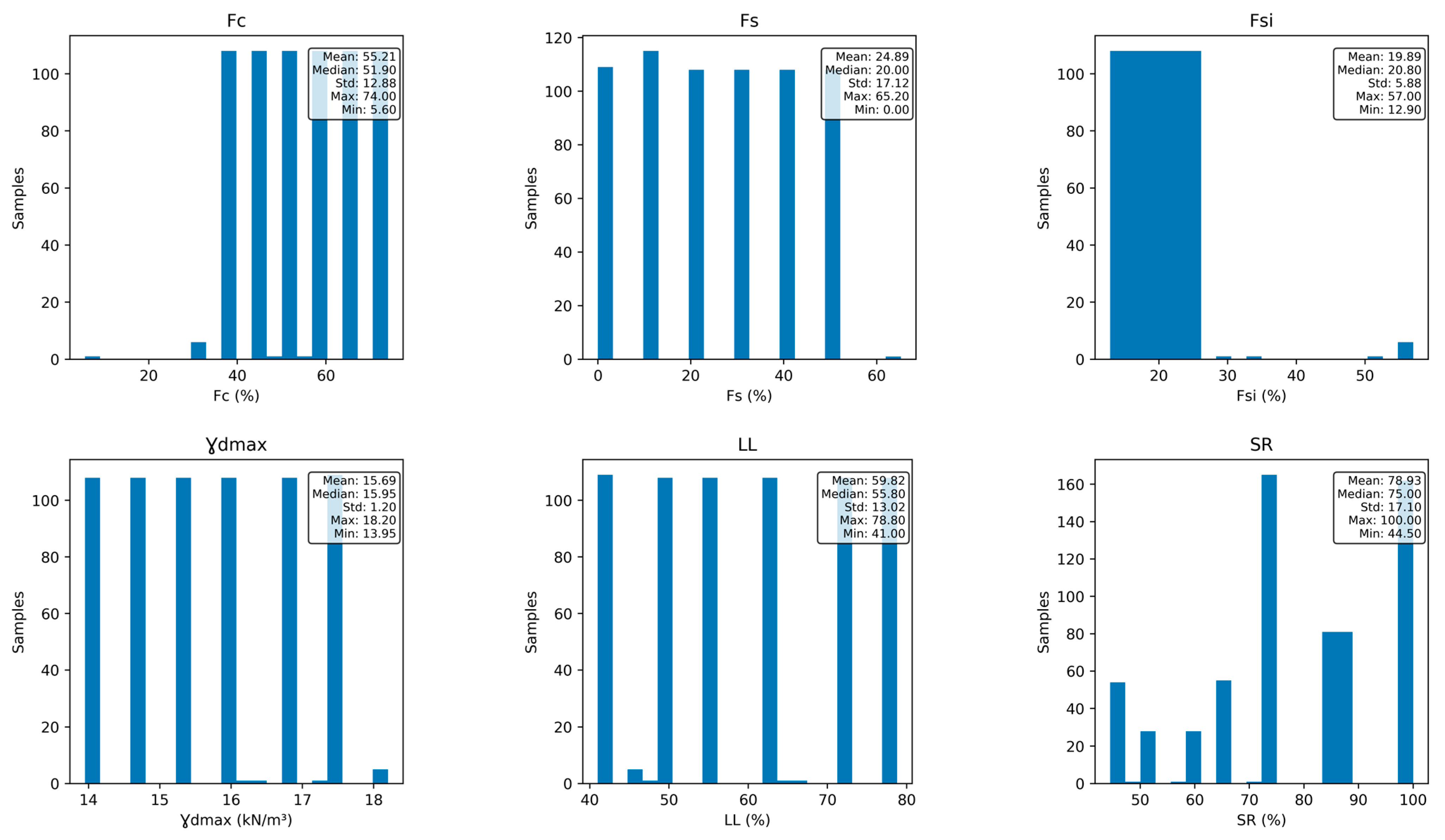
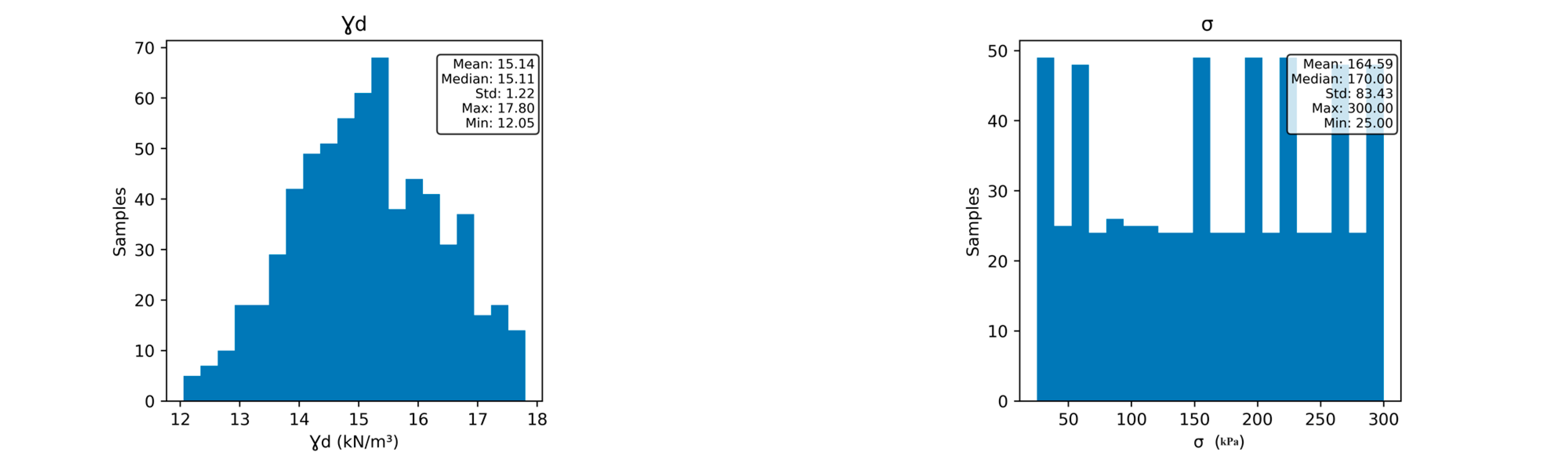
| LL (%) | SR (%) | (kN/m3) | (kN/m3) | Applied Stress [σ] (kN/m2) | |
|---|---|---|---|---|---|
| mean | 59.82 | 78.9 | 15.14 | 15.69 | 164.59 |
| std | 13.02 | 17.1 | 1.22 | 1.20 | 83.43 |
| min | 41.00 | 44.5 | 12.05 | 13.95 | 25.00 |
| 25% | 48.60 | 65.0 | 14.26 | 14.66 | 87.50 |
| 50% | 55.80 | 75.0 | 15.11 | 15.95 | 170.00 |
| 75% | 72.10 | 88.0 | 16.05 | 16.73 | 240.00 |
| max | 78.80 | 100.0 | 17.80 | 18.20 | 300.00 |
| Models to Predict Dry Unit Weight () | Models to Predict Applied Stress () | |||
|---|---|---|---|---|
| Parameters | Minimum | Maximum | Minimum | Maximum |
| Input parameters | Input parameters | |||
| LL (%) | 41 | 79 | 41 | 79 |
| SR (%) | 45 | 100 | 45 | 100 |
| σ (kN/m2) | 25 | 300 | ||
| (kN/m3) | 12 | 17.8 | ||
| 13.95 | 18.2 | 13.95 | 18.2 | |
| Output parameter | Output parameter | |||
| (kN/m3) | 12 | 17.8 | ||
| (kN/m2) | 25 | 300 | ||
| Model | Hyperparameter | Values Range | Optimal Values | |
|---|---|---|---|---|
| DTR | max_depth | 5 to 15 | 14 | 13 |
| min_samples_leaf | 1 to 5 | 1 | 1 | |
| min_samples_split | 1 to 5 | 3 | 1 | |
| RFR | max_depth | 5 to 15 | 14 | 10 |
| min_samples_leaf | 1 to 5 | 1 | 1 | |
| min_samples_split | 1 to 5 | 1 | 1 | |
| n_estimators | 50 to 150 | 110 | 130 | |
| GBR | subsample | 0.5 to 1 | 0.8 | 0.9 |
| n_estimators | 50 to 250 | 250 | 200 | |
| min_samples_split | 2 to 20 | 17 | 10 | |
| min_samples_leaf | 1 to 20 | 3 | 2 | |
| max_depth | 3 to 15 | 10 | 5 | |
| learning_rate | 0.01 to 0.4 | 0.1 | 0.2 | |
| XGBoost | colsample_bytree | 0.6 to 1 | 1 | 0.8 |
| learning_rate | 0.01 to 0.4 | 0.1 | 0.2 | |
| max_depth | 1 to 15 | 7 | 6 | |
| n_estimators | 50 to 250 | 200 | 200 | |
| subsample | 0.5 to 1 | 0.8 | 0.6 | |
| SVR | C | 0.1 to 10,000 | 1000 | 10 |
| epsilon | 0.001 to 100 | 10 | 0.01 | |
| kernel | linear, poly, rbf | rbf | rbf | |
| ANN | number of neurons in layer1 | 2 to 100 | 8 | 8 |
| number of neurons in layer2 | 2 to 100 | 56 | 56 | |
| learning_rate | 0.01 to 0.4 | 0.05 | 0.025 | |
| batch size | 10 to 50 | 16 | 12 | |
| hidden layers function | ReLU, tanh, linear, Sigmoid | ReLU | tanh | |
| linkage between the hidden layer and the ultimate output layer function | ReLU, tanh, linear, Sigmoid | linear | ReLU | |
| Algorithm | Metrics | ||||||||
|---|---|---|---|---|---|---|---|---|---|
| Training | Validation | Testing | rd (%) | Training | Validation | Testing | rd (%) | ||
| DTR | R2 | 0.995 | 0.9337 | 0.9372 | 5.8 | 1 | 0.9931 | 0.9845 | 1.6 |
| RMSE | 5.79 | 22.63 | 21.79 | 276.3 | 0 | 0.10344 | 0.158 | - | |
| MAE | 3.65 | 17.414 | 16.414 | 349.7 | 0 | 0.0816 | 0.0965 | - | |
| RFR | R2 | 0.9946 | 0.9698 | 0.9636 | 3.1 | 0.999 | 0.9937 | 0.9924 | 0.7 |
| RMSE | 5.975 | 15.273 | 16.6 | 177.8 | 0.0374 | 0.0985 | 0.111 | 196.8 | |
| MAE | 4.728 | 12.344 | 12.954 | 174.0 | 0.0244 | 0.0687 | 0.0696 | 185.2 | |
| GBR | R2 | 0.9997 | 0.9839 | 0.9789 | 2.1 | 0.999 | 0.9954 | 0.9954 | 0.4 |
| RMSE | 1.385 | 11.16 | 12.64 | 812.6 | 0.01 | 0.085 | 0.087 | 770.0 | |
| MAE | 1.017 | 8.332 | 9.172 | 801.9 | 0.0081 | 0.052 | 0.0463 | 471.6 | |
| XGBoost | R2 | 0.9999 | 0.9841 | 0.9856 | 1.4 | 0.9999 | 0.9985 | 0.9976 | 0.2 |
| RMSE | 0.932 | 11.1 | 10.43 | 1019.1 | 0.01 | 0.048 | 0.062 | 520.0 | |
| MAE | 0.7035 | 8.19 | 7.92 | 1025.8 | 0.0068 | 0.035 | 0.039 | 473.5 | |
| SVR | R2 | 0.9554 | 0.971 | 0.972 | 1.7 | 0.9967 | 0.9954 | 0.9936 | 0.3 |
| RMSE | 17.26 | 15.07 | 14.60 | 15.4 | 0.069 | 0.0836 | 0.102 | 47.8 | |
| MAE | 10.79 | 10.622 | 11.37 | 5.4 | 0.0237 | 0.0444 | 0.0488 | 105.9 | |
| ANN | R2 | 0.9946 | 0.994 | 0.9917 | 0.3 | 0.9963 | 0.9977 | 0.9954 | 0.1 |
| RMSE | 6.01 | 6.82 | 7.92 | 31.8 | 0.073 | 0.06 | 0.086 | 17.8 | |
| MAE | 4.625 | 5.085 | 5.872 | 27.0 | 0.051 | 0.048 | 0.061 | 19.6 | |
Disclaimer/Publisher’s Note: The statements, opinions and data contained in all publications are solely those of the individual author(s) and contributor(s) and not of MDPI and/or the editor(s). MDPI and/or the editor(s) disclaim responsibility for any injury to people or property resulting from any ideas, methods, instructions or products referred to in the content. |
© 2024 by the authors. Licensee MDPI, Basel, Switzerland. This article is an open access article distributed under the terms and conditions of the Creative Commons Attribution (CC BY) license (https://creativecommons.org/licenses/by/4.0/).
Share and Cite
Alnmr, A.; Ray, R.; Alzawi, M.O. A Novel Approach to Swell Mitigation: Machine-Learning-Powered Optimal Unit Weight and Stress Prediction in Expansive Soils. Appl. Sci. 2024, 14, 1411. https://doi.org/10.3390/app14041411
Alnmr A, Ray R, Alzawi MO. A Novel Approach to Swell Mitigation: Machine-Learning-Powered Optimal Unit Weight and Stress Prediction in Expansive Soils. Applied Sciences. 2024; 14(4):1411. https://doi.org/10.3390/app14041411
Chicago/Turabian StyleAlnmr, Ammar, Richard Ray, and Mounzer Omran Alzawi. 2024. "A Novel Approach to Swell Mitigation: Machine-Learning-Powered Optimal Unit Weight and Stress Prediction in Expansive Soils" Applied Sciences 14, no. 4: 1411. https://doi.org/10.3390/app14041411
APA StyleAlnmr, A., Ray, R., & Alzawi, M. O. (2024). A Novel Approach to Swell Mitigation: Machine-Learning-Powered Optimal Unit Weight and Stress Prediction in Expansive Soils. Applied Sciences, 14(4), 1411. https://doi.org/10.3390/app14041411