An Algorithm for Finding Optimal k-Core in Attribute Networks

Abstract

As a structural indicator of dense subgraphs, k-core has been widely used in community search due to its concise and efficient calculation. Many community search algorithms have been expanded on the basis of k-core. However, relevant algorithms often set k values based on empirical analysis of datasets or require users to input manually. Once users are not familiar with the graph network structure, they may miss the optimal solution due to an improper k setting. Especially in attribute social networks, characterizing communities with only k-cores may lead to a lack of semantic interpretability of communities. Consequently, this article proposes a method for identifying the optimal k-core with the greatest attribute score in the attribute social network as the target community. The difficulty of the problem is that the query needs to integrate both structural and textual indicators of the community while fully considering the diversity of attribute scoring functions. To effectively reduce computational costs, we incorporate the topological characteristics of the k-core and the attribute characteristics of entities to construct a hierarchical forest. It is worth noting that we name tree nodes in a way similar to pre-order traversal and can maintain the order of all tree nodes during the forest creation process. In such an attribute forest, it is possible to quickly locate the initial solution containing all query vertices and reuse intermediate results during the process of expanding queries. We conducted effectiveness and performance experiments on multiple real datasets. As the results show, attribute scoring functions are not monotonic, and the algorithm proposed in this paper can avoid scores falling into local optima. With the help of the attribute k-core forest, the actual query time of the Advanced algorithm has improved by two orders of magnitude compared to the BaseLine algorithm. In addition, the average F1 score of our target community has increased by 2.04 times and 26.57% compared to ACQ and SFEG, respectively.

1. Introduction

Graphs are often used to represent complex network structures containing large-scale entities, where vertices denote entities and edges illustrate relationships between entities. Common ones include co-authorship relationships in scholar networks [1], friend relationships in social networks [2,3], and protein reaction relationships in biological networks [4,5]. Dense subgraph search has attracted widespread attention from scholars, especially community search based on personalized query conditions such as query vertices and structural indicators. Unlike traditional community detection, community search can complete personalized search tasks, making the target subgraph easier to interpret. As an important community search model, k-core requires each node in the subgraph to have at least $k$ neighbors. Compared with clique, quasi-clique, densest subgraph, k-truss, etc., k-core has become the basis of many dense subgraph algorithm models and has been widely used in industry and academia due to its simple structure and efficient calculation.

Even though the k-core has a lot of advantages, we find that many algorithm models are overly idealized when attempting to determine the k value during query execution. Some take the median as $k$ for queries based on empirical analysis of the dataset, while others are manually specified by the user. It should be noted that different datasets show differences in terms of their characteristics. When employing different structural evaluation indicators such as independence, maximum density, and conductivity, the scoring trend may not necessarily be positively (or negatively) associated with $k$. As for manual assignment, its uncertainty is greater, and once users are not familiar with the network, the performance of the model will be greatly reduced. Therefore, this article aims to globally search for the optimal k-core containing the specified query vertices.

In addition, with the continuous improvement of sensor devices, entities’ semantic features have become richer, and attribute networks [6,7,8,9] have emerged. People are no longer satisfied with utilizing only structural features to characterize entity relationships in the target network. To improve the semantic interpretability of queries, many models have added attribute correlation evaluation indicators to compensate for semantic deficiencies in simple graphs. However, there is no unified attribute scoring function to evaluate the attribute correlation of subgraphs. Different algorithm models design different attribute rating functions for diverse networks and objectives. To adapt to more application scenarios, we extract the primary keys from different attribute scoring functions in order to grasp their essence.

Given the attribute graph, an attribute scoring function, a query vertex set, and a query attribute set, the goal of this article is to find a k-core that contains query vertices and has the highest attribute rating. This can directly solve the problem of missing the optimal solution due to improper k value selection and can also serve as the basis for other algorithm models. A basic algorithm is to find all k-cores containing query vertices, calculate scores one by one, and return the optimal solution. However, the large computational cost makes it unsuitable for large attribute graphs. Hence, this article proposes an algorithm for searching for the optimal k-core on the attribute networks, integrating structural and attribute indicators, and constructing an index forest, which can improve adaptability and speed. Our main contributions are as follows:

• Propose the idea of an attribute-optimal k-core. Since it is possible to miss the optimal solution by determining k through empirical analysis or manual selection, this article searches for the optimal k-core on an attribute graph as the target community to find the optimal solution to the problem.
• Propose the advanced query algorithm. Extract primary keys from commonly used attribute scoring functions to adapt to various scoring needs. Taking advantage of the nested nature of k-core, design bidirectional reachable tree nodes, improve the naming and storage methods of tree nodes, quickly locate tree nodes, and achieve reuse of the calculation process.
• We conducted numerous experiments on multiple ground-truth datasets. The experimental results on these datasets show that the Advanced algorithm can effectively avoid the scoring function falling into local optima. Its main time consumption is in forest creation, and the actual query time is improved by two orders of magnitude compared to BaseLine.

The rest of this paper is organized as follows: We review the related work in Section 2. Section 3 formally defines the model and proposes two algorithms. The experiments conducted and their results are presented in Section 4. Finally, in Section 5, we summarize the main work and discuss future research directions.

2. Related Work

k-core is the largest connected subgraph in a network, in which each node has a degree of no less than $k$. It was originally used in the social sciences to characterize network cohesion [10]. Core decomposition can be completed by removing the vertices of the minimum degree one by one, which is called the peeling algorithm [11,12]. High computational efficiency makes k-core the foundation of many algorithm models in dense subgraph mining and community search. Moreover, with the development of large-scale social networks, mining dense subgraphs based solely on structural compactness is no longer sufficient for meeting application requirements. Attribute graph searches [13,14,15,16,17,18,19,20,21] have gradually gained the attention of industry and academia.

The ACQ query model [16] attempts to identify the community that contains the specified query vertices on the attribute graph. It shares the most attributes with the query attribute set. In contrast to the previous community search model, ACQ enhances the semantic interpretability of the target community, but the user must specify the appropriate core number as the query condition. This is too idealistic to assume that the user can be able to select the appropriate $k$ value, which may result in the algorithm failing to find the optimal solution. As well, the query algorithm is only applicable to a single query vertex, and in the process of querying, the subset of attributes is enumerated one by one to calculate the community score, which is not suitable for social networks with rich attributes.

The target subgraph of the KCCS model [17] needs to contain all query attributes, and the query path that connects each vertex in the subgraph to the attribute must be as short as possible. VAC [18] simplifies the startup parameters of the attribute community query. Users only need to provide query nodes and an integer $k$ to limit the query range so that the quality of candidate communities can be evaluated according to various attributes of query nodes (such as geographical location and keyword attributes), which not only enriches the dimension of community attributes but also effectively avoids the risk of a rigorous query attribute set. Unfortunately, with regard to structural indicators, both KCCS and VAC models still require users to input an appropriate $k$ value, which makes them also subject to the dilemma of selecting a $k$ value.

The ATC model [19] emphasizes that a good attribute scoring function should reward such communities, i.e., the more query attributes covered, the higher the score, and the fewer nodes unrelated to query attributes, the higher the score. Consequently, the ATC model assigns different weights to attributes and develops a community scoring function on the basis of attribute weighting. The model employs k-truss, which is tighter than k-core, as the structural indicator, but it still does not avoid the user’s choice of $k$ value, which limits the application of this model.

Wang et al. [20] have shown that the traditional greedy algorithm may stop prematurely during the process of improving the community score and adopt the first local optimal solution to be the optimal global solution. Therefore, they propose an elastic expansion method for the greedy algorithm, which allows the scoring function to continue trial and error within a limited number of times (including the number of trials and errors and the threshold of score reduction) after finding the first local optimal solution. While this has effectively improved the accuracy of the greedy algorithm, it does not guarantee that global optimization will be achieved.

Chu et al. [22] for the first time highlight the dangers associated with manually specifying the $k$ value in the dense subgraph search problem and propose to find the optimal k-core globally to eliminate the uncertainty associated with manual selection and empirical analysis. For the purpose of adapting to a variety of structural evaluation indicators, they first extract the primary keys from the scoring function, then realize the optimal query algorithm in space and time by lightweight sorting of nodes and edges. Unfortunately, the model does global community detection on a simple graph and cannot perform personalized community searches based on query vertices and attributes, making the communities found inexplicable. Therefore, we study a variety of attribute scoring functions and then identify the optimal k-core in the attribute social network according to the query vertex set and attribute set specified by the user. Its attribute score is the greatest, which reflects the community’s good semantic characteristics. Table 1 summarizes the comparison of relevant models.

Table 1. A comparison of representative models on community detection (CD) and attribute community search (ACS).

Model	Topic	Participation Condition 1	Structural Cohesiveness	Attribute Function	Target Community
[16]	ACS	$q, S, k$	k-core	YES	local
[17]	ACS	$S, k$	k-core	YES	local
[18]	ACS	$Q, k$	k-truss	YES	local
[19]	ACS	$Q, S, k,d$	(k, d)-truss	YES	local
[20]	ACS	$Q, S$	ECOQUG	YES	local
[22]	CD	-	k-core	NO	global
Ours	ACS	$Q, S$	k-core	NO	global

¹ Participation conditions may be a vertex $q$, a query vertex set $Q$, a query keyword set $S$, or some positive integers $k$ and $d$.

3. Proposed Approach

3.1. Problem Formulation

The problem studied in this article is defined on an undirected attribute graph $G=\left(V,E,A\right)$, where $V,E,A$ represent the vertex set, edge set and attribute set, respectively. $n=\left|V\right|$ and $m=\left|E\right|$ are the number of vertices and edges, generally $m>n$. For $\forall v\in V$, $v$ is an entity. Pair $\left(u,v\right)\in E$ is an edge, implying that there is a certain relationship between entities $u$ and $v$ (such as co-authorship, friends, etc.). For each $v$, there is a set $A\left(v\right)$ representing the text attributes of entity $v$. Different entities may share common attributes, which means that they may have a certain semantic similarity in these attributes. Table 2 shows the main notations appearing throughout the remain text.

Table 2. Notations and meanings.

Notation	Meaning
$G=\left(V,E,A\right)$	$G$ is an undirected attribute graph, including the vertex set $V$, the edge set $E$, and the attribute set $A$.
$A\left(v\right)$	the attribute set of vertex $v$.
$V\left(H\right)$	$H$ is the subgraph of $G$, $V\left(H\right)$ is the vertex set of $H$.
$n\left(H\right)$	the number of vertices in $H$.
$core\left(v\right)$	the core number of vertex $v$.
$Core\left(H\right)$	the core number set of graph $H$.
$C_k$	a connected graph composed of vertices with $core\left(v\right)=k$
$V_w$	a vertex set with $w\in A\left(v\right)$
$N_i^t$	a tree node in attribute k-core forest
$bi{n}_k$	a list of tree nodes that can be restored to $C_k$

To clarify the problem to be solved and the algorithm presented in this article, it is necessary to introduce the relevant concepts first.

Definition 1 (k-core).

Given a graph $G$ and a positive integer $k$, the subgraph $H$ is called a k-core of $G$, denoted as $C_k$, if and only if $H$ is a maximum connected subgraph and $\forall v\in H$, $\mathit{deg}ree(v) \ge k$.

It is worth emphasizing that the k-core obtained by the classical Peeling algorithm may contain multiple connected subgraphs, some of which can be viewed as multiple kinds of k-cores. For example, in Figure 1, the subgraph composed of {4, …, 26} can be viewed as a 4-core in the past, which contains two connected subgraphs. But in this article, according to Definition 1, we consider the subgraph composed of vertex set {9, …, 14} as a separate 5-core, which is more appropriate in real-world application scenarios and more conducive to the subsequent creation of forests.

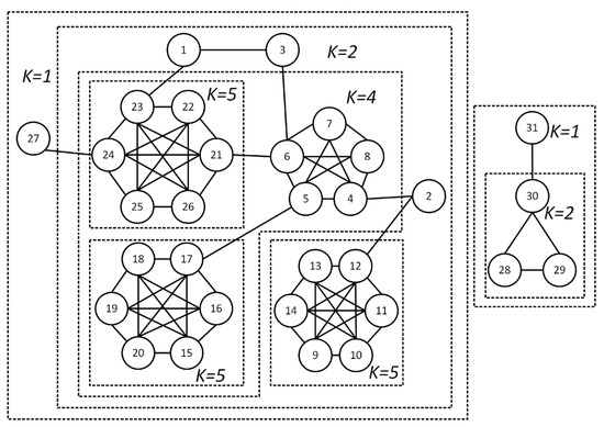
Figure 1. Sample network and its corresponding k-cores.

Definition 2 (core number).

For $\forall v \in G$, the core number of a vertex $v$ is $core\left(v\right)=max\left\{k\right|v\in C_k\}$, which is the maximum value of $k$ among all $C_k$ containing vertex $v$.

Generally, $k_{\mathit{max}}$ and $k_{\mathit{min}}$ are used to represent the maximum and minimum core number of the graph $G$, while $C_{k_{\mathit{max}}}$ represents the most tightly structured subgraph in graph $G$.

k-core can only characterize the compactness between vertices structurally, but for attribute graphs, each vertex has a different number of keywords to describe its characteristics. In order to achieve personalized queries and further explain the reasons for community formation, various attribute community search models have designed multiple attribute scoring functions [16,18,19,20,21] based on actual application scenarios to evaluate the quality of attribute communities.

Different models define attribute scoring functions differently, but they are usually derived from some primary keys. Assuming that $H$ is the subgraph to be evaluated and $S$ is the query attribute set, this article studies the following primary keys commonly used in attribute scoring functions:

• $V(H)$: the vertex set of subgraph $H$;
• $\mathrm{n}(H)$: the number of vertices in $H$, i.e., $\mathrm{n}(H)=\left|V(H)\right|$;
• $A(v)$: the attribute set of vertex $v$;
• $V_w$: the set of vertices in subgraph $H$ containing the attribute $w$;

Based on the above primary keys, some attribute scoring functions are defined as follows.

$$f\left(H,S\right)=\left|{\cap }_{v\in V\left(H\right)}\left(A\left(v\right)\cap S\right)\right|$$

(1)

Equation (1) determines the number of attributes shared by all vertices in subgraph $H$ with the query attribute set $S$.

$$f(H,S)={\displaystyle \sum _{w\in S}\frac{{\left|V_w\cap V(H)\right|}^2}{n(H)}}$$

(2)

First proposed by [19], Equation (2) determines the criteria that should be followed for the rating function of attribute communities. It is particularly pointed out that attributes have different contributions to community ratings, and the more vertices they are shared, the stronger the explanatory power of attributes on community semantics. Therefore, Equation (2) not only depends on the number of vertices containing the attribute $w$ but also considers the weight of the attribute $w$ in the subgraph $H$.

$$f(H,S)=\sqrt[\left|S\right|]{{\displaystyle \prod _{w\in S}\frac{{\left|V_w\cap V(H)\right|}^2}{n(H)}}}$$

(3)

Equation (3) is a modification of Equation (2), which rewards larger communities under the same conditions. That is, if each vertex of a large community covers most of the query attributes, it should receive a higher attribute score than its subgraph.

$$f(H,S)=\left\{\begin{array}{l}1,S\subseteq \left\{w|w\in \underset{v\in H}{\cup }A(v)\right\}\\ 0,others\end{array}\right.$$

(4)

As shown in Equation (4), some modes only require the target subgraph to cover all query attributes and then propose more requirements from different aspects, such as keyword distance [17], community diameter [21,23,24], similarity [18,25], which enriches application scenarios. Therefore, the goal of this article is to find the best k-core on the attribute graph that maximizes Equations (1)–(3). The formal problem definition is as follows:

Definition 3 (attribute optimal k-core).

Given an undirected attribute graph $G$, a query vertex set $Q$, a query attribute set $S$, and an attribute score function $f\left(H,S\right)$, for any $k_{\mathit{min}}\le k\le k_{\mathit{max}}$, if $C_k$ contains all query vertices in $Q$ and makes $f\left(H,S\right)$ optimal, then the subgraph $C_k$ is the attribute optimal k-core of $G$.

3.2. Algorithms for Finding the Optimal k-Core

To find the attribute optimal k-core, this section proposes two solutions, including the BaseLine algorithm and the Advanced algorithm, and analyzes their complexity.

3.2.1. BaseLine Algorithm

The BaseLine algorithm is easy to understand and implement, including the following steps:

• Step 1: Perform core decomposition on attribute graph $G$ to obtain the core numbers of all vertices.
• Step 2: For any $k_{\mathit{min}}\le k\le k_{\mathit{max}}$, select all vertices with $core\left(v\right)=k$ to construct all connected subgraphs as the candidate $C_k$ set.
• Step 3: Filter out the subgraphs uncovering the query node set $Q$ from the candidate $C_k$ set, and obtain the feasible solution $C_k$ set.
• Step 4: Calculate attribute scores for all feasible solution $C_k$, and return the subgraph with the best score as the optimal solution.

Performing core decomposition on the graph and constructing all $C_k$ based on the number of core vertices requires traversing all vertices and edges multiple times, which takes $O(k_{\mathit{max}}\ast (\left|V\right|+\left|E\right|))$ time. In the worst-case, if step 3 does not filter out any subgraphs, then attribute scores need to be calculated for all $C_k$. Let $O(F_k)$ be the time to compute the score of $C_k$, then the time complexity of the BaseLine algorithm is $O(k_{\mathit{max}}\ast (\left|V\right|+\left|E\right|)+{\displaystyle \sum _{k_{\mathit{min}}}^{k_{\mathit{max}}}{F}_k})$. Although the BaseLine algorithm is accurate and can finish in polynomial time, it is not user-friendly for large attribute networks.

3.2.2. Advanced Algorithm

We find that the performance bottleneck of the BaseLine algorithm lies in constructing $C_k$ for each $k_{\mathit{min}}\le k\le k_{\mathit{max}}$ and checking whether it contains the query vertex set $Q$. Most of the time, $Q$ may only exist in part of $C_k$, especially when the graph contains multiple connected subgraphs, resulting in more invalid computations. In addition, when $Q$ changes, the previous calculation result cannot be reused, and the feasible $C_k$ set needs to be filtered again, which is very unfavorable for online queries. Therefore, we deeply analysis the characteristics of the $C_k$ set and design a two-stage query algorithm:

• Stage 1: Utilize the nested nature of $C_k$ to construct a hierarchical attribute k-core forest and sort the tree nodes.
• Stage 2: Locate the query vertex set $Q$ to the relevant tree nodes, construct an initial feasible solution, and then gradually spread to the marginal tree nodes to find the optimal attribute $C_k$.

1.

Constructing the attribute k-core forest

According to Definition 1, for $k_{\mathit{min}}\le k_1<k_2\le k_{\mathit{max}}$, their corresponding k-cores are $C_{k_1}$ and $C_{k_2}$, respectively. If $C_{k_1}$ and $C_{k_2}$ belong to the same connected graph, then $C_{k_2}\subseteq C_{k_1}$, which is the nesting property of k-cores [26,27]. Trees can be used to organize and represent the relationships between different $C_k$. Combining the primary keys of these attribute scoring functions, we define the attribute $C_k$ tree node as follows.

Definition 4 (attribute k-core tree node).

For any $C_k$ in attribute graph $G$, there is a unique tree node $N_i^t$, where $t$ is the unique identifier of the tree and $i$ is the index number of the node in the tree. $N_i^t$ contains $parent$, $children$, $vertexSet$, and $invertedIndex$, which are, respectively used to identify its parent tree node, children tree nodes, connected k-shell vertex set, and the keyword inverted indexes in $vertexSet$.

Definition 5 (parent tree node).

Given the attribute graph $G$, for $k_{\mathit{min}}\le k_1<k_2\le k_{\mathit{max}}$, their k-cores are $C_{k_1}$ and $C_{k_2}$, respectively, and their tree nodes are represented by $N_{k_1}^t$ and $N_{k_2}^t$. If $N_{k_1}^t$ and $N_{k_2}^t$ belong to the same tree, $C_{k_2}\subseteq C_{k_1}$, and there is no $k_1<k^{*}<k_2$, then $N_{k_1}^t$ is the parent tree node of $N_{k_2}^t$.

Definition 6 (attribute k-core forest).

Given the attribute graph $G$, create attribute k-core tree nodes for each $k_{\mathit{min}}\le k\le k_{\mathit{max}}$. If the tree node has a parent tree node, then connect them. All trees form the attribute k-core forest.

It is important to note that $k$ may not be continuous, so a tree node’s core number does not necessarily equal its father tree node’s core number minus 1. As shown in Figure 2, subtrees with roots $N_1^0$ and $N_2^0$ can be restored to 2-core and 4-core, respectively. However, due to the lack of vertices with $core\left(v\right)=3$, $N_2^0$ becomes the legitimate child node of $N_1^0$, but their core numbers are not continuous. Furthermore, according to Definition 1, the subgraph composed of {9, …, 14} is actually a 5-core. So, although $N_2^0$ and $N_5^0$ are both child nodes of $N_1^0$, they are located at different $C_k$. Therefore, in the algorithm design for building attribute forest, we should only create tree nodes for the actual $k$ that exists, rather than all integer in $0\le k\le k_{\mathit{max}}$.

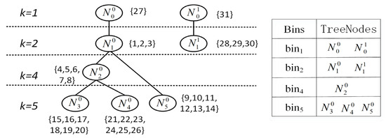
Figure 2. Hierarchical forest and the sorted tree nodes.

In order to quickly locate the tree node where the query vertex is located during the query phase, we store the tree node in a set of Bins. We organize Bins according to the following rules:

• If $core\left(v\right)$ of the connected k-shell set in $N_i^t$ equals $k$, then add $N_i^t$ to $bi{n}_k$.
• For tree nodes in the same $bi{n}_k$, sort them by tree number $t$ first. Then, for nodes belonging to the same tree, sort them by the minimum rank of vertices in the vertexSet.

So when locating the query vertex, we only need to search for the $bi{n}_k$ based on $core\left(v\right)$, and further locate its corresponding tree node with help of binary search algorithm. Note that if the located tree nodes belong to different trees, the query ends immediately because our target subgraph is at least a connected graph.

Algorithm 1 shows the pseudo-code for constructing a hierarchical forest. On the basis of core decomposition, hierarchical trees are constructed for each connected subgraph, finally resulting in a hierarchical forest. Lines 5, 6 create the root node of each tree, and line 7 recursively constructs its child nodes. Note that in Procedure $Build\_child\_node$, the tree nodes are numbered in the preorder traversal order. It also maintains $parent\_k$ and $child\_k$ during each recursive, which can avoid establishing blank tree nodes and reduces the storage cost of forests. In addition, the algorithm initially leaves bins empty and then creates a new $bi{n}_k$ when discovering an unclassified core number $k$. In other cases, only update the corresponding $bi{n}_k$. For a parent tree node, after all its child nodes are created, its attribute inverted index can be constructed as shown in line 10 of Procedure $Build\_child\_node$, since now all nodes in its $vertexSet$ belong to the same connected k-shell.

Algorithm 1 Building forest

Input: A graph $G=(V,E,A)$ Output: the hierarchical forest $Bins$ 1: $t\leftarrow 0$, $Bins\leftarrow \varnothing$ 2: compute $core\left(v\right)$ of each vertex in $G$ by core decomposition; 3: construct connected $Subgraphs$ from $G$; 4: for $graph$ in $Subgraphs$: 5:  $k_{\mathit{min}}\leftarrow \mathit{min}(core(v)) \mathrm{in} Core(graph)$, $node\_index\leftarrow 0$; 6:  create root tree node $N_{node\_index}^t$ and update $bi{n}_{k_{\mathit{min}}}$; 7:  $Build\_child\_node(N_{node\_index}^t,k_{\mathit{min}})$; 8:  update tree indicator $t$; 9: return $Bins$. Procedure $Build\_child\_node(parent\_node,parent\_k)$: 1: select vertices with $core\left(v\right)>parent\_k$ as candidate children vertex set; 2: if candidate children vertex set is not empty: 3:  obtain connected subgraphs composed of candidate vertex sets as $children\_graphs$; 4:  for each graph in $children\_graphs$: 5:   $node\_index\leftarrow node\_index+1$; 6:   select $\mathit{min}(core\left(v\right))$ in this graph as $child\_k$; 7:   create $child\_node$$N_{node\_index}^t$ and update $bi{n}_{child\_k}$; 8:   update $parent\_node$; 9:   $Build\_child\_node(child\_node,child\_k)$; 10: create attribute reverse index for $parent\_node$; 11: end $Build\_child\_node$

As shown in Figure 2, the hierarchical forest corresponding to the network in Figure 1 is composed of two trees, including a total of eight tree nodes. Starting from the root of the tree, as the depth increases, the core number of tree nodes gradually increases (not necessarily continuously), indicating an increasingly compact structure.

2.

Node localization and extended query

We apply the attribute hierarchical forest to the Advanced query algorithm, which consists of two parts: identifying the Lowest Common Ancestor node (LCA), and expanding the query, as shown in Algorithms 2 and 3.

Algorithm 2 LCA algorithm

Input: the hierarchical forest $Bins$, the query vertex set $Q$ Output: the lowest common ancestor $LCAncestor$ 1: $Nodelist\leftarrow \varnothing$, $i\_\mathit{min}\leftarrow None$, $i\_\mathit{max}\leftarrow None$ 2: for $v$ in $Q$: 3:  locate $bi{n}_k$ according $core\left(v\right)$; 4:  perform a binary search the tree node $N_i^t$, where $v \in N_i^t.vertexSet$; 5:  add $N_i^t$ to $Nodelist$; 6:  update $i\_\mathit{min}$$\mathrm{and} i\_\mathit{max}$; 7: end for 8: if the tree indicator $t$$\mathrm{of} N_i^t$$\mathrm{in} Nodelist$ are different: 9:  return $None$ # the query nodes do not belong to the same tree and have no common ancestor. 10: else: 11:  compute the lowest common ancestor for $N_{i\_\mathit{min}}^t$ and $N_{i\_\mathit{max}}^t$ as $LCAncestor$; 12: end if

According to the hierarchical tree construction process shown in Algorithm 1, the tree nodes are numbered in a preorder traversal manner, which endows the tree nodes with the following query properties.

Property 1.

For tree nodes $N_i^{t_1}$ and $N_j^{t_2}$, if $t_1\ne t_2$, then they do not belong to the same tree, that is, the vertices in their vertexSet are not connected.

Property 2.

For tree nodes $N_{i_1}^t$ and $N_{i_2}^t$, if $i_1<i_2$, then $N_{i_1}^t$ is created before $N_{i_2}^t$.

Property 3.

For tree nodes $N_{i_1}^t$, $N_i^t$, $N_{i_2}^t$, if $i_1<i<i_2$, then the LCA of $N_{i_1}^t$ and $N_{i_2}^t$ is also the LCA of all of them.

Firstly, the Algorithm 2 locates relevant tree nodes (see lines 3, 4) based on the core number of the query vertices, and records the minimum and maximum tree node index ($i\_\mathit{min}$ and $i\_\mathit{max}$, respectively). According to Property 1, if the located tree nodes do not belong to the same tree, the query ends prematurely. According to the Properties 2 and 3, the LCA of $N_{i\_min}^t$ and $N_{i\_max}^t$ is also the LCA of all tree nodes in $Nodelist$. Therefore, it is only necessary to perform a classic LCA search algorithm for $N_{i\_min}^t$ and $N_{i\_max}^t$ once. If you want it to be faster, you can consider a fast LCA algorithm. The subtree with the LCA node as the root node can be restored to the tightest subgraph containing all query vertices. Algorithm 3 takes it as the initial feasible solution and enters the expanding query stage to search for the optimal solution.

As shown in Figure 2, when $Q=\{4 , 9 , 16 , 25\}$, Algorithm 2 locates relevant tree nodes as $Nodelist=\left\{N_2^0, N_3^0, N_4^0, N_5^0\right\}$, $i\_\mathit{min}=2, i\_\mathit{max}=5$. Simply locating the LCA of $N_2^0$ and $N_5^0$ as $N_1^0$, which is also the ancestor of $N_3^0$ and $N_4^0$. The subtree rooted on $N_1^0$ can be restored to a connected 2-core, which is the initial feasible solution containing all query vertices.

Algorithm 3 Expanding query algorithm

Input: the hierarchical fores $Bins$, the query attribute set $S$, the attribute score function $f\left(H,S\right)$ and $LCAncestor$ Output: the optimal attribute k-core $C_{best}$ 1: $V(H)\leftarrow \varnothing$, $V_w\leftarrow \varnothing$, $C_{best}\leftarrow None$, $score\_best\leftarrow None$ 2: initialize $V(H)$, $V_w$ by traversing the subtree rooted in $LCAncestor$; 3: $score\_best\leftarrow$ compute $f(H,S)$ with $V(H)$ and $V_m$; 4: $C_{best}\leftarrow H$; 5: $finished\_subtree\leftarrow LCAncestor$; 6: while $finished\_subtree.parent$ exists: 7:  $current\_root\leftarrow finished\_subtree.parent$; 8:  if $current\_root$ has more than a child tree node: 9:     for each $child$ in $current\_root.children$ but not the $finished\_subtree$: 10:   traverse the subtree rooted on $child$ in pre-order, and iteratively update primary keys $V(H)$$, V_w$; 11:   compute $score$ of $H$; 12:   if $score$ is better than $score\_best$: 13:      update $score\_best$, $C_{best}$; 14:  $finished\_subtree\leftarrow current\_root$; 15: return $C_{best}$

In Algorithm 3, the primary keys and optimal solution $C_{best}$ are first initialized with the subtree rooted in $LCAncestor$, as shown in lines 2–4. If $LCAncestor$ is not the root of the tree, then we take its parent tree node as $current\_root$ and enter the expansion phase. Note that the subtree rooted on $LCAncestor$ has completed the calculation of the primary keys and can be recorded as $finished\_subtree$ (line 5). Subsequently, only other child subtrees of $current\_root$ will be traversed. The traversal process continuously updates the primary keys, and only calculates the score of the new graph when tracing back to $current\_root$, as shown in lines 9–13. After that, we update $finished\_subtree$ again and continue to expand upward until the root of the tree to obtain the optimal solution $C_{best}$.

Assuming $Q=\{4, 16, 25\}$, according to Algorithm 2, the $LCAncestor$ is located as $N_2^0$, that is, the initial feasible solution is $C_4$. According to Algorithm 3, since $N_2^0$ is not the root of the tree, it needs to be extended upward to the $N_1^0$ node to calculate subgraph $C_2$. Note that $N_1^0$ has two child nodes, but $N_2^0$ has already completed the calculation. It only needs to visit $N_5^0$, update $V\left(H\right)$ and $V_w$, and complete the calculation of the 2-core score when going back to $N_1^0$. In the same way, continue to expand to $N_0^0$ and calculate the score of $C_1$. At this time, $C_{best}$ is obtained.

Although the time of the Advanced algorithm can be divided into two parts: forest creation and extended query, once the hierarchical forest is created, it only needs dynamic maintenance [28]. Therefore, the main query time depends on the depth of $LCAncestor$. The greater the depth, the more iterations and the longer the time. Since Algorithm 3 computes scores only on the ancestor path of $LCAncestor$, the statistical results of primary keys can be reused, the query time will be significantly reduced.

4. Experiments and Results

In this part, multiple experiments are designed to verify the effectiveness and efficiency of the proposed algorithms. In order to find the optimal attribute k-core, we implement the BaseLine and Advanced algorithms for the attribute scoring functions (see Equations (1)–(3)) listed in Section 3.1.

The datasets in the experiments are shown in Table 3, where $A\left(V\right)$ is the number of unique attributes in the dataset, $\overline{A\left(v\right)}$ is the average number of attributes per vertex, and $k_{\mathit{max}}$ is the maximum core number of the dataset. Each dataset contains several high-quality ground-truth communities and attributes. In particular, for the Facebook dataset, which contains 10 different heterogeneous networks. For convenience of expression, we use $F_X$ to represent the heterogeneous network centered on vertex $X$, such as F414. The Facebook dataset can be obtained from SNAP, and the Twitter and Flickr datasets are quoted from the literature [29,30].

Table 3. Statistics of datasets.

Dataset	$\mathit{n}$	$\mathit{m}$	$\mathit{A}\left(\mathit{V}\right)$	$\overline{\mathit{A}\left(\mathit{v}\right)}$	${\mathit{k}}_{\mathit{max}}$
Twitter	2403	3715	9067	15	59
Facebook	4039	88,234	1283	9	115
Flickr	7575	239,738	12,047	24	93

For the fairness and effectiveness of the experiment, we selected the top 10 ground-truth communities with the largest scale from each dataset for querying. For each community to be evaluated, select the top 30% of attributes that appear the most frequently and are different from other communities as their representative attributes. The F1 score is used as an evaluation indicator when evaluating community quality. By default, the number of query vertexes is 12, and the query attributes are all representative attributes of a community. A single-factor evaluation method is employed to evaluate the impact of parameters on the model.

4.1. Evaluating the Effectiveness of Algorithms

We refer to the subgraph containing all query vertices as a feasible solution. In order to observe the ratings of different k-cores as comprehensively as possible, we identify the most tightly structured ground-truth communities. By executing the BaseLine algorithm and recording the scores of all feasible solutions, Table 4 shows the optimal k-core with different scoring functions. Note that $f_1$, $f_2$, and $f_3$, respectively, represent the scoring functions shown in Equations (1)–(3).

Table 4. Best k for different attribute scoring functions.

	F0	F107	F348	F414	F686	F698	F1684	F1912	F3437	F3980	Twitter	Flickr
$f_1$	18	69	29	23	19	8	39	109	19	7	49	85
$f_2$	16	63	24	18	7	6	37	70	16	5	38	73
$f_3$	20	66	26	19	9	9	41	72	20	7	51	89

As can be seen from Table 4, for the same query conditions, the optimal k-core is quite different when adopting different attribute scoring functions. Figure 3 shows the rating curves of networks F107, F348, F1684, F1912, Twitter, and Flickr when adopting Equation (3). The results illustrate that the same scoring function has different trends on different datasets, and there are many local optimal solutions. This fully demonstrates that determining the k value by manual selection or dataset analysis cannot guarantee global optimality, which also means that the problem proposed in this article is necessary.

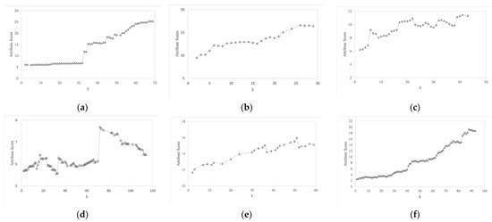
Figure 3. Attribute scoring of k-cores on different datasets. (a) F107 (b) F348 (c) F1684 (d) F1912 (e) Twitter (f) Flickr.

4.2. Evaluating the Performance of Algorithms

The time of the BaseLine algorithm includes core decomposition and score computation, while the time of the Advanced algorithm additionally includes building the forest. We have calculated the execution time of each part, which helps identify the efficiency bottleneck of the algorithm. Since multiple heterogeneous networks on Facebook differ significantly in scale, only the query times of a few larger heterogeneous networks are displayed here, as shown in Figure 4.

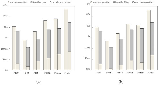
Figure 4. Runtime of algorithms on different datasets. (a) Runtime with Equation (1) (b) Runtime with Equation (2).

The experimental results show that regardless of the datasets, the Advanced algorithm is always faster than the BaseLine algorithm. Upon careful observation of the time consumption at different stages of the algorithm, we find that in the BaseLine algorithm, score calculation accounts for the largest proportion of time. This is consistent with theoretical analysis since the BaseLine algorithm must calculate the score of every feasible solution, and the calculation process cannot be shared. As for the Advanced algorithm, building a hierarchical forest costs the most time. The actual query time includes two parts: locating the LCA for query vertices and extending queries. With the excellent properties of attribute tree nodes and iterative updates of primary keys, the Advanced algorithm’s computation time is greatly reduced. If the forest construction time is not taken into account, the Advanced algorithm is two orders of magnitude faster than the BaseLine algorithm. By dynamically maintaining the forest, the Advanced algorithm can achieve millisecond-level online queries.

4.3. Estimating the Quality of Communities

In order to evaluate the quality of the target community discovered by the Advanced algorithm, we compare it with the communities queried by the ACQ and SFEG algorithms. This is because ACQ uses k-core as the structural indicator and constructs a k-shell tree for the entire graph, which is similar to our forest; SFEG proposes an elastic mechanism to alleviate premature stopping of greedy algorithms, which expands the applicability of local optimal solutions.

As shown in Figure 5, our target community quality is superior to that of ACQ and SFEG. The reason is that ACQ only supports one query vertex. When the query vertex set has multiple vertices, ACQ randomly selects one of them as the query vertex. Especially in large attribute networks, the attribute density of vertices is higher, coupled with overlapping communities, leading to poorer query performance, such as in Flickr. Although the SFEG algorithm supports multiple query nodes, it still requires manually specifying the challenge threshold for the greedy algorithm. This makes it unable to avoid falling into local optima.

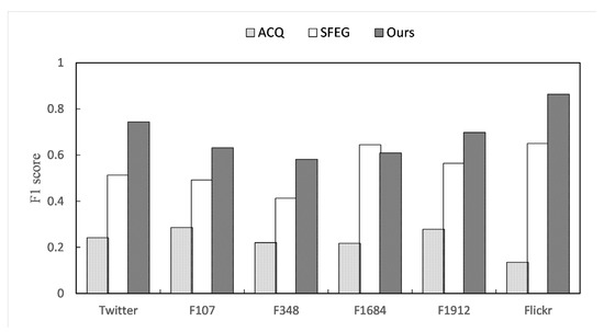
Figure 5. Community quality on different datasets.

4.4. Parameter Sensitivity

This section evaluates the impact of query vertices and query attributes on algorithm efficiency and effectiveness through experiments. As mentioned earlier, after the forest construction is complete, the Advanced query algorithm only includes two stages: LCA (Algorithm 2) and Expand (Algorithm 3). This section will illustrate how parameters Q and S affect the efficiency of the Advanced algorithm and the quality of the target community.

As shown in Figure 6, the larger the query attribute set, the longer it takes to calculate the score, as there are more primary keys to calculate. The attribute density of a dataset also affects query time. In Flickr, $\overline{A\left(v\right)}$ = 24.5, while in F1684, $\overline{A\left(v\right)}$ = 7.85, which leads to a significant difference in the number of representative attributes of the ground-truth community. The higher the attribute density of the dataset, the more representative it contains, and the longer the average query time. The more representative attributes a query attribute set contains, the more accurately the community can be queried.

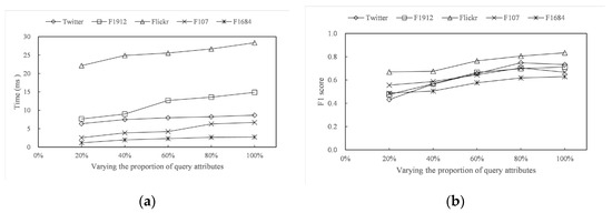
Figure 6. Varying query attributes. (a) Time with different attributes (b) F1 score with different attributes.

Figure 7a shows that the more query vertices there are, the more related tree nodes can be located, and the distribution may be broader as well. More importantly, the depth of their common ancestors may be shallower, which to some extent reduces the query time. Nevertheless, the core number of vertices in the dataset has a significant impact on query time. For example, despite its smaller size, F1912 has a much higher $k_{\mathit{max}}$ and average degree than Twitter, resulting in more query iterations and longer query times. Too many query vertices can lead to excessive dispersion of related tree nodes, large community size, and mixing with low-quality vertices. Especially in loosely structured networks, such as F1684 in Figure 7b, LCA is too close to the tree root, resulting in a loss of community quality.

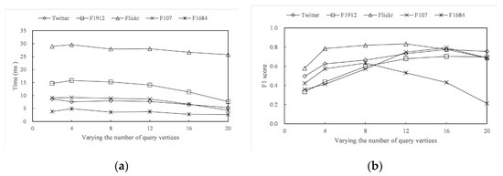
Figure 7. Varying query vertices. (a) Time with different vertices (b) F1 score with different vertices.

Overall, the algorithm proposed in this article can quickly find the globally optimal k-core for the target community. But the experiment conducted in this article is based on high-quality, large-scale communities in datasets. If applied to development scenarios, the model’s accuracy will be affected. Additionally, it is necessary to design stable and efficient algorithms to maintain attribute forests in dynamic network graphs, which will be the model’s future improvement direction.

5. Conclusions

The aim of this article is to find the attribute optimal k-core community within the attribute network in order to overcome the problem that empirical analysis and manual selection of k values may miss the optimal solution. Hence, we propose the concept of global optimal attribute k-core and design the BaseLine algorithm. To address the bottleneck of the BaseLine algorithm, we have constructed a hierarchical k-core forest that integrates structural and attribute semantic indicators and utilizes k-core’s nested nature. The attribute forest can transform complex graph problems into classical tree operations, reducing the difficulty of queries. Based on attribute forests, we have developed a two-stage advanced algorithm. It can locate the LCA of all relevant tree nodes at once and iteratively update the primary keys during the extended query stage, recycling the intermediate calculation process. Several experiments on real datasets show that the attribute optimal k-core is primarily affected by the scoring function, the query vertices, and the query attributes. Excluding the time required to create the forest, the advanced algorithm is two orders of magnitude faster than the BaseLine algorithm. In terms of community quality, the target community is significantly better than ACQ and SFEG. In order to improve the effectiveness and efficiency of the algorithm in the future, we will further adapt more attribute scoring functions and optimize the forest maintenance method for dynamic graphs.

References

- Li, C.; Tang, Y.; Xiao, Z.; Li, T. Influential scholar recommendation model in academic social network. J. Comput. Appl. 2020, 40, 6. [Google Scholar]
- Sozio, M.; Gionis, A. The community-search problem and how to plan a successful cocktail party. In Proceedings of the 16th ACM SIGKDD International Conference on Knowledge Discovery and Data Mining, Washington, DC, USA, 25–28 July 2010; pp. 939–948. [Google Scholar]
- Leskovec, J.; Mcauley, J. Learning to discover social circles in ego networks. Adv. Neural Inf. Process. Syst. 2012, 25, 539–547. [Google Scholar]
- Palla, G.; Derényi, I.; Farkas, I.; Vicsek, T. Uncovering the overlapping community structure of complex networks in nature and society. Nature 2005, 435, 814–818. [Google Scholar] [CrossRef] [PubMed]
- Cui, W.; Xiao, Y.; Wang, H.; Lu, Y.; Wang, W. Online search of overlapping communities. In Proceedings of the 2013 ACM SIGMOD International Conference on Management of Data, New York, NY, USA, 22–27 June 2013; pp. 277–288. [Google Scholar]
- Zhu, Q.; Hu, H.; Xu, C.; Xu, J.; Lee, W.C. Geo-social group queries with minimum acquaintance constraints. VLDB J. 2017, 26, 709–727. [Google Scholar] [CrossRef]
- Xie, X.; Song, M.; Liu, C.; Zhang, J.; Li, J. Effective influential community search on attributed graph. Neurocomputing 2021, 444, 111–125. [Google Scholar] [CrossRef]
- Sun, H.; Huang, R.; Jia, X.; He, L.; Sun, M.; Wang, P.; Sun, Z.; Huang, J. Community search for multiple nodes on attribute graphs. Knowl.-Based Syst. 2020, 193, 105393. [Google Scholar] [CrossRef]
- Lin, P.; Yu, S.; Zhou, X.; Peng, P.; Li, K.; Liao, X. Community search over large semantic-based attribute graphs. World Wide Web 2022, 25, 927–948. [Google Scholar] [CrossRef]
- Seidman, S.B. Network structure and minimum degree. Soc. Netw. 1983, 5, 269–287. [Google Scholar] [CrossRef]
- Batagelj, V.; Zaversnik, M. An o (m) algorithm for cores decomposition of networks. arXiv 2003, arXiv:cs/0310049. [Google Scholar]
- Liu, B.; Zhang, F. Incremental algorithms of the core maintenance problem on edge-weighted graphs. IEEE Access 2020, 8, 63872–63884. [Google Scholar] [CrossRef]
- Chowdhary, A.A.; Liu, C.; Chen, L.; Zhou, R.; Yang, Y. Finding attribute diversified community over large attributed networks. World Wide Web 2022, 25, 569–607. [Google Scholar] [CrossRef]
- Ghosh, B.; Ali, M.E.; Choudhury, F.M.; Apon, S.H.; Sellis, T.; Li, J. The flexible socio spatial group queries. Proc. VLDB Endow. 2018, 12, 99–111. [Google Scholar] [CrossRef]
- Islam, M.S.; Ali, M.E.; Kang, Y.B.; Sellis, T.; Choudhury, F.M.; Roy, S. Keyword aware influential community search in large attributed graphs. Inf. Syst. 2022, 104, 101914. [Google Scholar] [CrossRef]
- Fang, Y.; Cheng, C.K.; Luo, S.; Hu, J. Effective community search for large attributed graphs. Proc. VLDB Endow. 2016, 9, 1233–1244. [Google Scholar] [CrossRef]
- Zhang, Z.; Huang, X.; Xu, J.; Choi, B.; Shang, Z. Keyword-centric community search. In Proceedings of the 2019 IEEE 35th International Conference on Data Engineering (ICDE), Macao, China, 8–11 April 2019; IEEE: Piscataway, NJ, USA, 2019; pp. 422–433. [Google Scholar]
- Liu, Q.; Zhu, Y.; Zhao, M.; Huang, X.; Xu, J.; Gao, Y. VAC, vertex-centric attributed community search. In Proceedings of the 2020 IEEE 36th International Conference on Data Engineering (ICDE), Dallas, TX, USA, 20–24 April 2020; IEEE: Piscataway, NJ, USA, 2020; pp. 937–948. [Google Scholar]
- Huang, X.; Lakshmanan, L.V.S. Attribute truss community search. arXiv 2016, arXiv:1609.00090. [Google Scholar]
- Wang, C.; Wang, H.; Chen, H.; Li, D. Attributed community search based on effective scoring function and elastic greedy method. Inf. Sci. 2021, 562, 78–93. [Google Scholar] [CrossRef]
- Luo, J.; Cao, X.; Xie, X.; Qu, Q.; Xu, Z.; Jensen, C.S. Efficient attribute-constrained co-located community search. In Proceedings of the 2020 IEEE 36th International Conference on Data Engineering (ICDE), Dallas, TX, USA, 20–24 April 2020; IEEE: Piscataway, NJ, USA, 2020; pp. 1201–1212. [Google Scholar]
- Chu, D.; Zhang, F.; Lin, X.; Zhang, W.; Zhang, Y.; Xia, Y.; Zhang, C. Finding the best k in core decomposition, A time and space optimal solution. In Proceedings of the 2020 IEEE 36th International Conference on Data Engineering (ICDE), Dallas, TX, USA, 20–24 April 2020; IEEE: Piscataway, NJ, USA, 2020; pp. 685–696. [Google Scholar]
- Guo, T.; Cao, X.; Cong, G. Efficient algorithms for answering the m-closest keywords query. In Proceedings of the 2015 ACM SIGMOD International Conference on Management of Data, Victoria, Australia, 31 May–4 June 2015; pp. 405–418. [Google Scholar]
- Wang, K.; Wang, S.; Cao, X.; Qin, L. Efficient radius-bounded community search in geo-social networks. IEEE Trans. Knowl. Data Eng. 2020, 34, 4186–4200. [Google Scholar] [CrossRef]
- Luo, J.; Cao, X.; Xie, X.; Qu, Q. Best co-located community search in attributed networks. In Proceedings of the 28th ACM International Conference on Information and Knowledge Management, Beijing, China, 3–7 November 2019; pp. 2453–2456. [Google Scholar]
- Matula, D.W.; Beck, L.L. Smallest-last ordering and clustering and graph coloring algorithms. JACM 1983, 30, 417–427. [Google Scholar] [CrossRef]
- Sariyuce, A.E.; Seshadhri, C.; Pinar, A.; Catalyurek, U.V. Finding the hierarchy of dense subgraphs using nucleus decompositions. In Proceedings of the 24th International Conference on World Wide Web, Florence, Italy, 18–22 May 2015; pp. 927–937. [Google Scholar]
- Lin, Z.; Zhang, F.; Lin, X.; Zhang, W.; Tian, Z. Hierarchical core maintenance on large dynamic graphs. Proc. VLDB Endow. 2021, 14, 757–770. [Google Scholar] [CrossRef]
- He, T.; Liu, Y.; Ko, T.H.; Chan, K.C.; Ong, Y.S. Contextual correlation preserving multiview featured graph clustering. IEEE Trans. Cybern. 2019, 50, 4318–4331. [Google Scholar] [CrossRef] [PubMed]
- He, T.; Bai, L.; Ong, Y.S. Vicinal vertex allocation for matrix factorization in networks. IEEE Trans. Cybern. 2021, 52, 8047–8060. [Google Scholar] [CrossRef] [PubMed]
Disclaimer/Publisher’s Note: The statements, opinions and data contained in all publications are solely those of the individual author(s) and contributor(s) and not of MDPI and/or the editor(s). MDPI and/or the editor(s) disclaim responsibility for any injury to people or property resulting from any ideas, methods, instructions or products referred to in the content. |
© 2024 by the authors. Licensee MDPI, Basel, Switzerland. This article is an open access article distributed under the terms and conditions of the Creative Commons Attribution (CC BY) license (https://creativecommons.org/licenses/by/4.0/).