A Simple Model for Estimating the Hydraulic Conductivity of Unsaturated Soil

Abstract

Describing the hydraulic conductivity of unsaturated soil is very important in predicting water transport. Most current models have complex forms and generally need to be calibrated by the measured unsaturated hydraulic conductivity curve. A simple model, by which it is possible to conveniently predict the unsaturated hydraulic conductivity, is proposed in this study. The soil–water characteristic curve and hydraulic conductivity curve are separated into three parts. The soil–water characteristic curve is represented by Fredlund and Xing’s equation. A simple model composed of three lines is proposed for estimating the hydraulic conductivity of unsaturated soil. The model parameters can be conveniently calibrated from the measured soil–water characteristic curve and saturated hydraulic conductivity. Finally, the proposed model is validated by the experimental data from different soils. The proposed model provides a simple approach to estimating the hydraulic conductivity of unsaturated soil, which is more convenient for practical application.

1. Introduction

Geotechnical problems and geological hazards at the earth’s surface are often closely related to water transport through soils, such as rainfall-induced settlements and landslides [1,2,3,4]. The majority of the natural soils are generally unsaturated [5]. Hence, a reasonable description of the hydraulic conductivity of unsaturated soils is critical to accurately predicting the water movement [6,7].

A direct measurement of the unsaturated hydraulic conductivity is the most accurate method. The commonly used methods include horizontal infiltration, outflow, evaporation and instantaneous profile [8]. However, these methods are time-consuming and costly, especially for a low water content [9]. Therefore, numerous studies have proposed models for estimating the unsaturated hydraulic conductivity. The majority of these models (including empirical, macroscopic and statistical models) have been established by bridging the soil–water characteristic curve (SWCC) with the hydraulic conductivity curve [10]. The statistical models are the most widely used ones, being based on the capillary flow and free-associative pores [9,11,12]. Childs and Collis-George [13] proposed the Childs and Collis-George model in terms of the Kelvin capillary model and the Hagen–Poiseuille equation. Since then, various statistical models have been proposed [6,14,15,16,17,18,19,20]. However, the construction of these models was based on the capillary flow in the low suction range. Thus, they cannot describe the situation where the adsorptive water film flow dominates for the high suction range [21,22].

To improve the estimation of the hydraulic conductivity, which is dominated by an adsorptive water film flow in the high suction range, Tokunaga [23,24] derived a hydraulic conductivity model based on the planar thin film dynamics. Since this model has explicit physical meaning, many studies have combined it with statistical models to predict the hydraulic conductivity over a wide suction range [25,26,27,28,29,30,31]. Lebeau and Konrad [25] adopted the Mualem model to account for the capillary flow, and constructed a new equation for calculating the adsorptive water flow which included the effects of ionic-electrostatic forces and molecular forces. Wang et al. [26,27,28] used the hydraulic conductivity at the critical suction point as a reference in simplifying the model of water film flow, and they also used the Mualem model to calculate the capillary flow. Gou et al. [31] proposed a more precise model accounting for the adsorptive water film based on micromechanics, and they used the Mualem model to predict the capillary flow as well. These models have a good ability to estimate the hydraulic conductivity over a wide suction range. However, the forms of these models are relatively complex. Additionally, these models used the Mualem model with scaling parameters, which need to be determined by the measured unsaturated hydraulic conductivity curve. These obstacles limit the application of these models in practice.

This study aims to propose a simple and convenient hydraulic conductivity model for unsaturated soil. Firstly, the soil–water interaction mechanisms are explained, and accordingly, the soil–water characteristic curve and hydraulic conductivity curve are divided into three parts. Secondly, Fredlund and Xing’s equation is used to describe the soil–water characteristic curve. Thirdly, a simple piecewise function is proposed for estimating the hydraulic conductivity of unsaturated soil. Fourthly, a calibration approach for the model parameters is introduced. Finally, the performance of the proposed model is validated with experimental data from different soils.

2. Methods

2.1. Soil-Water Interaction Mechanisms

Two distinct soil–water interaction mechanisms exist in unsaturated soil: capillarity and adsorption. The capillarity results from the difference between the inner water pressure and the outer air pressure (as caused by the surface tension), and the adsorption stems from four interactions involving the water film and the soil particles: electric double layer, van der Waals, and the surface and cation hydration potentials [31]. The electric double layer and van der Waals potential are commonly known as ionic-electrostatic and molecular potential, respectively [25]. The residual suction is generally regarded as the boundary between the capillarity and adsorption. Accordingly, the soil–water characteristic curve (SWCC) and the hydraulic conductivity curve can be divided into the capillary and adsorptive dominant regions [26,32]. Furthermore, due to the different shapes of the capillary water, the capillary dominating region can be separated into the boundary effect zone and the transition zone [33]. Figure 1 shows the soil–water interaction mechanisms, a typical soil–water characteristic curve and a hydraulic conductivity curve.

When the suction is smaller than the air-entry value, almost all pores in the soil are water-filled, and the soil falls within the boundary effect zone. In the boundary effect zone, the hydraulic conductivity is only slightly reduced, as compared with the saturated one. As the suction further increases, the filled water in the large pores becomes discharged and replaced by air, a large amount of pendular water appears between the soil particles, and the soil enters the transition zone. Many previous studies have shown that the hydraulic conductivity in the transition zone decreases almost linearly with the suction in the log–log scale [11,25,31]. As the suction exceeds the residual one, the water in the soil mainly exists in the form of an adsorptive water film, and the adsorption will dominate the soil–water interactions in this range. In this adsorptive dominant region, the thickness of the water film decreases with increasing suction, and the hydraulic conductivity is recognized to be decreasing linearly with increasing suction in the log–log scale as well [26,29,30]. In addition, when the suction is smaller than the transition suction Ψ_f, the hydraulic conductivity is entirely dependent on the capillary flow [31].

2.2. Soil-Water Characteristic Curve Model

An accurate description of the soil–water characteristic curve over a wide suction range is the basis for the estimation of the hydraulic conductivity. Many SWCC models have been proposed [34]. A four-parameter SWCC equation was proposed by Fredlund and Xing [35], which can effectively describe the SWCC over the wide suction range by introducing a correction function. Fredlund and Xing’s equation, in terms of suction (Ψ) and degree of saturation (S_r), is written as follows:

$$S_r={\displaystyle \frac{C(\psi )}{{\left\{\ln \left[e+{\left({\displaystyle \frac{\psi }{\alpha }}\right)}^n\right]\right\}}^m}}$$

(1)

$$C\left(\psi \right)=1-{\displaystyle \frac{\ln \left(1+{\displaystyle \frac{\psi }{C_r}}\right)}{\ln \left(1+{\displaystyle \frac{{10}^6}{C_r}}\right)}}$$

(2)

where e is the natural constant; α is a parameter that is related to the air-entry value; m and n are parameters that are associated with the SWCC shape; C(Ψ) is the correction function; C_r is not the precise residual suction value. It is more reasonable to consider C_r as a fitting parameter that is associated with the residual suction [36].

2.3. A Simple Model for Estimating the Hydraulic Conductivity of Unsaturated Soil

According to the soil–water interaction analysis, the hydraulic conductivity curve of unsaturated soil is divided into the boundary effect zone, transition zone and adsorptive dominant region by four critical points including the minimum suction at measurable saturation, air-entry value, residual suction and the highest suction. Specifically, the hydraulic conductivity in the boundary effect zone decreases slightly compared with the saturated one. Furthermore, the hydraulic conductivities of the transition zone and the adsorptive dominant region decrease approximately linearly on the log–log scale with different slopes. Consequently, the hydraulic conductivity curve can be simplified as three straight lines (Figure 2), and a simple piecewise model of the hydraulic conductivity is proposed as follows:

$$\begin{array}{l}\log k_w=\log k_{wa}+{\displaystyle \frac{\log \psi -\log {\psi }_a}{\log {\psi }_s-\log {\psi }_a}}(\log k_s-\log k_{wa})\hspace{1em}\hspace{1em}\mathrm{for} \psi \le {\psi }_{\mathrm{a}}\\ \log k_w=\log k_{wr}+{\displaystyle \frac{\log \psi -\log {\psi }_r}{\log {\psi }_{\mathrm{a}}-\log {\psi }_r}}(\log k_{wa}-\log k_{wr})\hspace{1em}\hspace{1em}\mathrm{for} {\psi }_{\mathrm{a}}<\psi \le {\psi }_r\\ \log k_w=\log k_{wm}+{\displaystyle \frac{\log \psi -\log {\psi }_m}{\log {\psi }_r-\log {\psi }_m}}(\log k_{wr}-\log k_{wm})\hspace{1em}\hspace{1em}\mathrm{for} \psi >{\psi }_r\end{array}$$

(3)

where Ψ_s, Ψ_a, Ψ_r and Ψ_m are the minimum suction at measurable saturation, air-entry value, residual suction and the highest suction (i.e., 10⁶ kPa), respectively. k_s, k_wa, k_wr and k_wm are the permeabilities corresponding to the suctions of Ψ_s, Ψ_a, Ψ_r and Ψ_m. The saturated hydraulic conductivity is commonly obtained by direct measurements using constant head tests or falling head tests. The critical step is to determine the values of k_wa, k_wr and k_wm.

Soil pores are almost water-filled in the boundary effect zone, and the hydraulic conductivity in this zone decreases slightly compared with the saturated one. For simplicity, it is suggested that the filled-water flow in this zone follows Darcy law. Thus, the hydraulic conductivity is proportional to the water cross-section area per unit area of the soil. Furthermore, the length of the water flow path is assumed to be invariable in the boundary effect zone, so the degree of saturation is equal to the ratio of the water cross-section area at an unsaturated state to that at a completely saturated state. Accordingly, the variation in the degree of saturation can be used to represent the variation in the water cross-section area, which can approximately characterize the change in the hydraulic conductivity in this zone. Hence, the hydraulic conductivity that corresponds to the air-entry value can be estimated by Equation (4):

$$k_{wa}=S_{ra}{k}_s$$

(4)

where k_wa is the hydraulic conductivity at Ψ_a; k_s is the saturated hydraulic conductivity; S_ra represents the degree of saturation at Ψ_a, whose expression is as follows:

$$S_{ra}={\displaystyle \frac{1-{\displaystyle \frac{\ln \left(1+{\psi }_a/C_r\right)}{\ln \left(1+{10}^6/C_r\right)}}}{{\left\{\ln \left[e+{\left({\psi }_a/\alpha \right)}^n\right]\right\}}^m}}$$

(5)

where a, m, n and C_r are model parameters in Fredlund and Xing’s equation; and e is the natural constant.

Furthermore, according to Lebeau and Konrad [25] and Gou et al. [31], the capillary component and adsorptive component in Figure 1b intersect roughly at the residual suction, which indicates that the hydraulic conductivity at the residual suction is approximately double the size of the adsorptive component. Additionally, Figure 1b shows that the hydraulic conductivity at very high suction depends almost entirely on the adsorptive water flow. Therefore, the hydraulic conductivities k_wr and k_wm can be determined by the adsorptive water flow as follows:

$$k_{wr}=2k_{ar}$$

(6)

$$k_{wm}=k_{am}$$

(7)

where k_wr and k_wm are hydraulic conductivities at the residual and maximum suction; k_ar is the adsorptive component of the hydraulic conductivity at the residual suction; and k_am is the adsorptive component of the hydraulic conductivity corresponding to the maximum suction.

A classic hydraulic conductivity model of the adsorptive water film flow proposed by Tokunaga [23,24] is adopted to calculate the adsorptive component of the hydraulic conductivity, which is presented as follows:

$$k_a=\frac{4{\rho }_{w}g}{\pi {\mu }_w}\frac{1-n^{\prime }}{d_e}{f}^3$$

(8)

where k_a is the adsorptive component of the permeability; ρ_w is the water density, ρ_w = 1000 kg/m³; μ_w denotes the water viscosity, μ_w = 1.005 × 10⁻³ Pa·s; g denotes the gravity acceleration, g = 9.8 m/s²; n’ is the porosity; d_e is the equivalent diameter for soil particles; and f denotes the thickness of the adsorptive water film. Equation (8) shows that the key to estimating the adsorptive component of the hydraulic conductivity is to determine the thickness of the adsorptive water film f and the equivalent diameter for soil particles d_e.

The thickness of the adsorptive water film is mainly dependent on the potential of the adsorptive water film. For a planar thin water film, its potential at the high suction is approximated by the disjointing pressure, which is considered to be identical to the suction [37]. Although the potential of the adsorptive water film includes four components, only the ionic-electrostatic (i.e., electric double layer) and molecular (i.e., van der Waals) potentials are considered in the studies of the thin water film flow [25,38], which can be expressed by the following equations [39,40]:

$${\mathsf{\Pi }}_m=-\frac{A_{svl}}{6\pi }\frac{1}{f^3}$$

(9)

$${\mathsf{\Pi }}_e=\frac{\epsilon {\epsilon }_0}{2}{\left(\frac{\pi k_{B}T}{ze}\right)}^2\frac{1}{f^2}$$

(10)

where Π_m denotes the molecular potential; Π_e denotes the ionic-electrostatic potential; f denotes the thickness of the adsorptive water film; ε denotes the static relative permittivity of water, ε = 78.54; ε₀ denotes the permittivity of free space, ε₀ = 8.85 × 10⁻¹² C²·J⁻¹·m⁻¹; T denotes the Kelvin temperature, T = 293.15 K; k_B denotes the Boltzmann constant, k_B = 1.381 × 10⁻²³ J/K; z denotes the ion charge, z = 1; A_svl denotes the Hamaker constant, A_svl = −6 × 10⁻²⁰ J in this study; and e denotes the electron charge, e = 1.602 × 10⁻¹⁹ C.

Furthermore, the ratio of the molecular potential to the ionic-electrostatic potential for various adsorptive water film thicknesses has been calculated and is presented in Figure 3. The molecular potential, Π_m, is found to be much higher than the ionic-electrostatic potential, Π_e, for a very thin water film. However, the value of Π_m/Π_e decreased rapidly for an increase in water film thickness, and the ionic-electrostatic potential becomes much larger than the molecular potential for a relative thick water film. This variation in P_m/P_e with adsorptive water film thickness is consistent with the results reported by Lu and Zhang [37]. Since the adsorptive water film thickness increases with a decreasing suction, for simplicity, it is suggested that the potentials of the adsorptive water film at the residual suction and the highest suction are approximated by the ionic-electrostatic potential and the molecular potential, respectively. Therefore, according to Equations (9) and (10), the adsorptive water film thicknesses at the residual suction and at the highest suction can be expressed as follows:

$$f_r=\sqrt{\frac{\epsilon {\epsilon }_0}{2}}\left(\frac{\pi k_{B}T}{ze}\right)\frac{1}{\sqrt{{\psi }_r}}$$

(11)

$$f_m={\left(-\frac{A_{svl}}{6\pi {\psi }_m}\right)}^{\frac{1}{3}}$$

(12)

where f_r is the thickness of adsorptive water film at the residual suction Ψ_r; and f_m is the thickness of adsorptive water film at the maximum suction Ψ_m.

In addition, Lebeau and Konrad [25] derived the expression of the equivalent diameter of the soil particles. The specific surface area of the polydisperse sample can be estimated in terms of the soil–water characteristic data at high suction as follows [21]:

$$A_s=\frac{n^{\prime }{S}_{rm,m}}{1-n^{\prime }}{\left(-\frac{A_{svl}}{6\pi {\psi }_{m,m}}\right)}^{-\frac{1}{3}}$$

(13)

where A_s is the specific surface area; n’ is the porosity; A_svl is the Hamaker constant; Ψ_m,m is the suction value, which corresponds to the situation where the capillary condensation caused by surface roughness is negligible, which is approximately taken as 10⁴ kPa [21]; and S_rm,m is the degree of saturation at Ψ_m,m, which can be calculated in the following equation:

$$S_{rm,m}={\displaystyle \frac{1-{\displaystyle \frac{\ln \left(1+{\psi }_{m,m}/C_r\right)}{\ln \left(1+{10}^6/C_r\right)}}}{{\left\{\ln \left[e+{\left({\psi }_{m,m}/\alpha \right)}^n\right]\right\}}^m}}$$

(14)

Furthermore, the specific surface area of the monodisperse sample composed of the identical spherical particles is approximated by 6/d_e [25]. Assuming the polydisperse sample has the same specific surface area as the monodisperse sample, then the expression of the equivalent diameter of the polydisperse sample can be derived as follows [25]:

$$d_e=\frac{6(1-n^{\prime })}{n^{\prime }}{\left(-\frac{A_{svl}}{6\pi {\psi }_{m,m}}\right)}^{\frac{1}{3}}\frac{1}{S_{rm,m}}$$

(15)

As a consequence, combining Equations (6)–(8) and (11)–(15), equations for the hydraulic conductivities at the residual suction and at the highest suction are obtained as follows:

$$k_{wr}=\left[\frac{4{\rho }_{w}g}{3\pi {\mu }_w}{\left(\frac{\epsilon {\epsilon }_0}{2}\right)}^{1.5}{\left(\frac{\pi k_{B}T}{ze}\right)}^3{\left(-\frac{A_{svl}}{6\pi {\psi }_{m,m}}\right)}^{-\frac{1}{3}}\right]\left(n^{\prime }{\psi }_r^{-1.5}{S}_{rm,m}\right)$$

(16)

$$k_{wm}=\left[\frac{2{\rho }_{w}g}{3\pi {\mu }_w}\left(-\frac{A_{svl}}{6\pi {\psi }_m}\right){\left(-\frac{A_{svl}}{6\pi {\psi }_{m,m}}\right)}^{-\frac{1}{3}}\right]\left(n^{\prime }{S}_{rm,m}\right)$$

(17)

where k_wr and k_wm are hydraulic conductivities at the residual and maximum suction. Notably, the parameters in the brackets […] of Equations (16) and (17) are generally considered to be constants. Therefore, these equations can be furthermore simplified to the following formulas:

$$k_{wr}=1.962\times {10}^{-2}\left(n^{\prime }{\psi }_r^{-1.5}{S}_{rm,m}\right)$$

(18)

$$k_{wm}=9.647\times {10}^{-15}\left(n^{\prime }{S}_{rm,m}\right)$$

(19)

As a consequence, by substituting Equations (4), (18) and (19) into Equation (3), a simple hydraulic conductivity model is achieved.

$$\begin{array}{l}\log k_w=\log \left(S_{ra}{k}_s\right)+{\displaystyle \frac{\log \left(\psi /{\psi }_a\right)}{\log \left({\psi }_s/{\psi }_a\right)}}\left[\log \left(1/S_{ra}\right)\right]\hspace{1em}\hspace{1em}\hspace{1em}\hspace{1em}\hspace{1em}\hspace{1em}\hspace{1em}\hspace{1em}\hspace{1em}\hspace{1em}\hspace{1em}\hspace{1em}\hspace{1em}\hspace{1em}\hspace{1em}\hspace{1em}\hspace{1em}\mathrm{for} \psi \le {\psi }_{\mathrm{a}}\\ \log k_w=\log \left[1.962\times {10}^{-2}\left(n^{\prime }{\psi }_r^{-1.5}{S}_{rm,m}\right)\right]+{\displaystyle \frac{\log \left(\psi /{\psi }_r\right)}{\log \left({\psi }_a/{\psi }_r\right)}}\left\{\log \left[{\displaystyle \frac{S_{ra}{k}_s}{1.962\times {10}^{-2}\left(n^{\prime }{\psi }_r^{-1.5}{S}_{rm,m}\right)}}\right]\right\}\hspace{1em}\mathrm{for} {\psi }_{\mathrm{a}}<\psi \le {\psi }_r\\ \log k_w=\log \left[9.647\times {10}^{-15}\left(n^{\prime }{S}_{rm,m}\right)\right]+{\displaystyle \frac{\log \left(\psi /{\psi }_m\right)}{\log \left({\psi }_r/{\psi }_m\right)}}\left\{\log \left[{\displaystyle \frac{1.962\times {10}^{-2}\left({\psi }_r^{-1.5}\right)}{9.647\times {10}^{-15}}}\right]\right\}\hspace{1em}\hspace{1em}\hspace{1em}\hspace{1em}\hspace{1em}\mathrm{for} \psi >{\psi }_r\end{array}$$

(20)

where the porosity n′ is a fundamental physical parameter; S_ra and S_rm,m can be calculated by Equations (5) and (14); Ψ_m,m is commonly set to be 10⁴ kPa; Ψ_s is commonly set to 0.01 kPa, 0.1 kPa or 1 kPa representing the minimum suction of the measured SWCC. The air-entry value Ψ_a and the residual suction y_r can be conventionally calibrated by the measured SWCC. This proposed model can, thus, predict the hydraulic conductivity of unsaturated soil over a wide suction range. Moreover, it is unnecessary to calibrate the scaling parameter by the measured unsaturated hydraulic conductivity curve.

2.4. Parameter Calibration

Four parameters of the SWCC model in this study need to be calibrated, including a, m, n and C_r. These parameters can be easily determined by fitting the measured SWCC with the least-squares method. In addition, three parameters in the proposed hydraulic conductivity model should be calibrated, including the saturated hydraulic conductivity k_s, the air-entry value Ψ_a and the residual suction Ψ_r. The saturated hydraulic conductivity k_s can be easily measured by the conventional constant head test or falling head test. In the present study, an approach for the calibration of Ψ_a and Ψ_r has been developed based on the studies by Zhai and Rahardjo [41,42].

As can be seen in Figure 1a, Ψ_a is generally considered to be the intersection of the horizontal line corresponding to the saturated state and the tangent line through the inflection point. Also, the residual suction is generally determined by the intersection of the tangent line through the inflection point with the straight line through the SWCC at the high suction [41,42]. The horizontal line corresponding to the saturated state is easily determined as follows:

$$S_r=1.0$$

(21)

The inflection point is the point with the maximum slope of SWCC (in the logarithmic scale), which also corresponds to the zero value of the second-order derivative of SWCC. Hence, the suction of the inflection point can be obtained by solving Equation (22):

$$\frac{d^2{S}_r}{d{\left(\log \psi \right)}^2}=\ln \left(10\right)\psi \left[\frac{d^2{S}_r}{d{\psi }^2}\ln \left(10\right)\psi +\frac{d{S}_r}{d\psi }\ln \left(10\right)\right]=0$$

(22)

Since the correction function C(Ψ) mainly affects the high suction range, it is reasonable to use the three parameters of Fredlund and Xing’s equation without any correction function for the resolution of the inflection point suction, which greatly simplifies the solution of Equation (22). By substituting Fredlund and Xing’s equation without any correction function into Equation (22), a simplified equation can here be obtained:

$$\frac{m+1}{\ln \left[e+{\left(\psi /\alpha \right)}^n\right]}\frac{{\left(\psi /\alpha \right)}^n}{e+{\left(\psi /\alpha \right)}^n}+\frac{{\left(\psi /\alpha \right)}^n}{e+{\left(\psi /\alpha \right)}^n}-1=0$$

(23)

where a, m, n and C_r are model parameters in Fredlund and Xing’s equation; and e is the natural constant.

By replacing the term $e+{\left(\psi /\alpha \right)}^n$ by t, Equation (23) can be simplified as:

$$\left(m+1\right)\left(t-e\right)-e\ln t=0$$

(24)

Equation (24) can then be easily solved using the Newton iteration method, with at most five iterative steps. The inflection point suction Ψ_f is, thereby, obtained.

Furthermore, the slope of the tangent line through a point of SWCC (in a semi-logarithmic coordinate) can be derived as follows:

$${\displaystyle \frac{d{S}_r}{d\left(\log \psi \right)}}=-\psi \ln \left(10\right)\left\{{\displaystyle \frac{{\left\{\ln \left[e+{\left(\psi /\alpha \right)}^n\right]\right\}}^{-m}}{C_r\left(1+\psi /C_r\right)\ln \left(1+{10}^6/C_r\right)}}+{\displaystyle \frac{mn{\left(\psi /\alpha \right)}^{n-1}\left[1-{\displaystyle \frac{\ln \left(1+\psi /C_r\right)}{\ln \left(1+{10}^6/C_r\right)}}\right]}{\alpha \left[e+{\left(\psi /\alpha \right)}^n\right]{\left\{\ln \left[e+{\left(\psi /\alpha \right)}^n\right]\right\}}^{m+1}}}\right\}$$

(25)

By substituting the value of Ψ_f in Equations (1), (2) and (25), the degree of saturation and the slope of the tangent line at the inflection point can be obtained by Equations (26) and (27):

$$S_{rf}=\frac{1-{\displaystyle \frac{\ln \left(1+{\psi }_f/C_r\right)}{\ln \left(1+{10}^6/C_r\right)}}}{{\left[\ln \left(e+1\right)\right]}^m}$$

(26)

$${\displaystyle \frac{d{S}_{rf}}{d\left(\log {\psi }_f\right)}}=-{\psi }_f\ln \left(10\right)\left\{{\displaystyle \frac{{\left[\ln \left(e+{\left({\psi }_f/\alpha \right)}^n\right)\right]}^{-m}}{C_r\left(1+{\psi }_f/C_r\right)\ln \left(1+{10}^6/C_r\right)}}+{\displaystyle \frac{mn\left[1-{\displaystyle \frac{\ln \left(1+{\psi }_f/C_r\right)}{\ln \left(1+{10}^6/C_r\right)}}\right]}{\alpha \left[e+{\left({\psi }_f/\alpha \right)}^n\right]{\left[\ln \left(e+{\left({\psi }_f/\alpha \right)}^n\right)\right]}^{m+1}}}\right\}$$

(27)

where S_rf is the degree of saturation at the inflection suction Ψ_f; and dS_rf/d(logΨ_f) is the slope of the tangent line at the inflection point Ψ_f. Moreover, the tangent line through the inflection point can be expressed by Equation (28):

$$S_r=S_{rf}+\frac{d{S}_{rf}}{d\left(\log {\psi }_f\right)}\left(\log \psi -\log {\psi }_f\right)$$

(28)

As suggested by Zhai and Rahardjo [41,42], the straight line of the SWCC at the high suction is determined by the suction of 3000 kPa. By substituting Ψ = 3000 kPa in Equations (1), (2) and (25), the expression of this straight line can then be obtained as follows:

$$S_r=S_{r3000}+\frac{d{S}_{r3000}}{d\left(\log {\psi }_{3000}\right)}\left(\log \psi -\log 3000\right)$$

(29)

$$S_{r3000}={\displaystyle \frac{1-{\displaystyle \frac{\ln \left(1+3000/C_r\right)}{\ln \left(1+{10}^6/C_r\right)}}}{{\left\{\ln \left[e+{\left(3000/\alpha \right)}^n\right]\right\}}^m}}$$

(30)

$${\displaystyle \frac{d{S}_{r3000}}{d\left(\log {\psi }_{3000}\right)}}=-3000\ln \left(10\right)\left\{{\displaystyle \frac{{\left\{\ln \left[e+{\left(3000/\alpha \right)}^n\right]\right\}}^{-m}}{C_r\left(1+3000/C_r\right)\ln \left(1+{10}^6/C_r\right)}}+{\displaystyle \frac{mn{\left(3000/\alpha \right)}^{n-1}\left[1-{\displaystyle \frac{\ln \left(1+3000/C_r\right)}{\ln \left(1+{10}^6/C_r\right)}}\right]}{3000\left[e+{\left(3000/\alpha \right)}^n\right]{\left\{\ln \left[e+{\left(3000/\alpha \right)}^n\right]\right\}}^{m+1}}}\right\}$$

(31)

where S_r3000 is the degree of saturation at the suction of 3000 kPa and dS_r3000/d(logΨ₃₀₀₀) is the slope of the tangent line at the suction of 3000 kPa. Furthermore, by combining Equations (20), (27) and (28), expressions for y_a and y_r are formed:

$${\psi }_a={\psi }_f{10}^{\left[\frac{1-S_{rf}}{d{S}_{rf}/d\left(\log {\psi }_f\right)}\right]}$$

(32)

$${\psi }_r={10}^{\left[\frac{S_{rf}-S_{r3000}-\frac{d{S}_{rf}}{d\left(\log {\psi }_f\right)}\log {\psi }_f+\frac{d{S}_{r3000}}{d\left(\log {\psi }_{3000}\right)}\log 3000}{\frac{d{S}_{rf}}{d\left(\log {\psi }_f\right)}+\frac{d{S}_{r3000}}{d\left(\log {\psi }_{3000}\right)}}\right]}$$

(33)

where Ψ_a, Ψ_r and Ψ_f are the air-entry value, residual suction and inflection point, respectively; S_rf and S_r3000 are the degree of saturations at the inflection suction and the suction of 3000 kPa; dS_rf/d(logΨ_f) and dS_r3000/d(logΨ₃₀₀₀) are the slopes of the tangent lines at the inflection point and the suction of 3000 kPa.

3. Results

In this section, the hydraulic conductivities of different soils have been estimated by using the proposed hydraulic conductivity model. The experimental data of different soils were collected from previous studies. The porosities, saturated hydraulic conductivities and references of these soils are presented in

Table 1. Soil porosities, saturated permeabilities and references of experimental data.

Soil Name	Reference	Porosity	Saturated Hydraulic Conductivity
		n’	ks (m/s)
Berlin medium sand	Nemes et al. [44]	0.388	7.30 × 10−5
Booischot loamy sand	Nemes et al. [44]	0.437	1.42 × 10−7
Helecine silt loam	Nemes et al. [44]	0.443	6.30 × 10−7
Sandy loam	Pachepsky et al. [45]	0.43	9.26 × 10−7
Clay loam	Pachepsky et al. [45]	0.5	7.52 × 10−8
Gilat loam	Mualem [46]	0.44	2.0 × 10−6
Yan’an loess (silty clay)	Tian et al. [7]	0.47	6.43 × 10−7

. Also, the validation of the proposed model has been evaluated by using the coefficient of determination (R²) for the estimated values versus experimental data. R² has been widely used to evaluate the quality of fitting of models in practice, and its expression is presented as follows [43]:

$$R^2=1-\frac{{{\displaystyle \sum _{i=1}^N\left[\log k_{wi}-\log {\widehat{k}}_{wi}\right]}}^2}{{{\displaystyle \sum _{i=1}^N\left[\log k_{wi}-\log {\overline{k}}_{wi}\right]}}^2}$$

(34)

where N is the number of experimental data points; ${\widehat{k}}_{wi}$ and k_wi are the estimated and measured hydraulic conductivities corresponding to the experimental data point i; and ${\overline{k}}_{wi}$ is the average of the measured hydraulic conductivities. The closer the value of R² is to 1, the better the predictive effect of the model.

In the present study, the detailed calculation procedure is as follows: (i) the measured SWCC is fitted by Equations (1) and (2), and the parameters of the SWCC model are obtained; (ii) the values of Ψ_a and Ψ_r are calculated by Equations (21)–(33); (iii) by substituting the suctions of Ψ_a and Ψ_m,m in Equations (5) and (14), their corresponding degree of saturation (S_ra and S_rm,m) can be calculated; (iv) the estimated hydraulic conductivity is acquired by substituting the parameters n′, S_ra, S_rm,m, Ψ_m,m, Ψ_s, Ψ_a, Ψ_r and k_s in Equation (20). The fitted parameters of the SWCC for the different soils are presented in

Table 2. Fitted parameters of the SWCC for the different soils.

Soil Name	a	m	n	Cr	Ψs (kPa)	Ψa (kPa)	Ψr (kPa)	Ψm,m (kPa)	Sra (%)	Srm,m (%)
Berlin medium sand	3.715	0.432	69.32	10.578	0.1	2.65	5.16	10,000	93.5	2.64
Booischot loamy sand	6.6	0.443	4.567	4.225	0.1	4.59	22.88	10,000	91.4	7.85
Helecine silt loam	3.416	0.523	0.828	6.209	0.1	0.59	179.76	10,000	92.4	14.29
Sandy loam	13.195	1.417	1.114	1.6 × 105	0.1	3.37	133.48	10,000	90	5.7
Clay loam	40.609	0.843	0.652	330.225	0.1	8.2	1344.87	10,000	90.5	19.08
Gilat loam	4.832	0.323	7.888	2.811	0.1	3.83	11.84	10,000	91.6	9.59
Yan’an loess (silty clay)	10.82	1.273	1.386	1.65 × 1016	1	3.784	87.641	10,000	90.4	5.66

.

As shown in Figure 4, the R² values are larger than 0.98 and the fitted SWCCs are highly consistent with the experimental data, which verifies the good applicability of Fredlund and Xing’s equation to different soils. Figure 5 shows the estimated hydraulic conductivities together with the corresponding experimental data. It can be seen that the measured hydraulic conductivity curves of different soils are approximately in the form of three segments, which are consistent with the proposed hydraulic conductivity model. Note that the inflection points of estimated hydraulic conductivities are almost exactly coincident with the experimental results, which indicates that the proposed parameters calibration method can accurately determine the air-entry value and residual suction and proves again that it is reasonable to divide the hydraulic conductivity curve by air-entry value and residual suction. Furthermore, it can be seen that the estimated hydraulic conductivities agree quite well with the experimental data, with an R² value larger than 0.83. This good agreement exists throughout the whole suction range. This result demonstrates a good performance of the proposed model in the estimation of the hydraulic conductivity of sand, silt and clay over a wide suction range. Moreover, it can be seen that even though the suction range of the measured SWCCs is relatively small, the estimated hydraulic conductivity curve also shows good agreement with the experimental data over the wide suction range. For example, Figure 5g shows a well-estimated hydraulic conductivity curve in the whole suction range, while the suction of measured SWCC in Figure 4g is less than 300 kPa.

4. Discussion

In the present study, based on the analysis of the soil–water interaction mechanisms over a wide suction range, a simple model for estimating the hydraulic conductivity of unsaturated soil has been proposed. The results have demonstrated that the proposed model has a good ability to estimate the hydraulic conductivity of different unsaturated soils with satisfactory accuracy. Compared with existing approaches, the proposed model has a simpler form composed of three straight lines. Furthermore, all parameters of the proposed model can be conveniently calibrated by the measured SWCC and saturated hydraulic conductivity, and it is unnecessary to calibrate the scaling parameter by the measured unsaturated hydraulic conductivity curve as the existing approaches [30]. Therefore, the proposed model can more conveniently estimate the hydraulic conductivity of unsaturated soil over a wide suction range, which will facilitate the application of unsaturated seepage in practice.

The estimation accuracy of the proposed model is associated with the determination of the air-entry value and residual suction based on the measured SWCC. The parameters calibration approach in this study mainly focuses on the unimodal SWCC, which cannot determine the residual suction of the bimodal SWCC. Additionally, this study does not consider the influence of hydraulic hysteresis on the hydraulic conductivity. Further studies on these aspects are needed in the future.

5. Conclusions

A simple model for estimating the hydraulic conductivity of unsaturated soil has been proposed in the present study, and the main conclusions are summarized below.

(1)

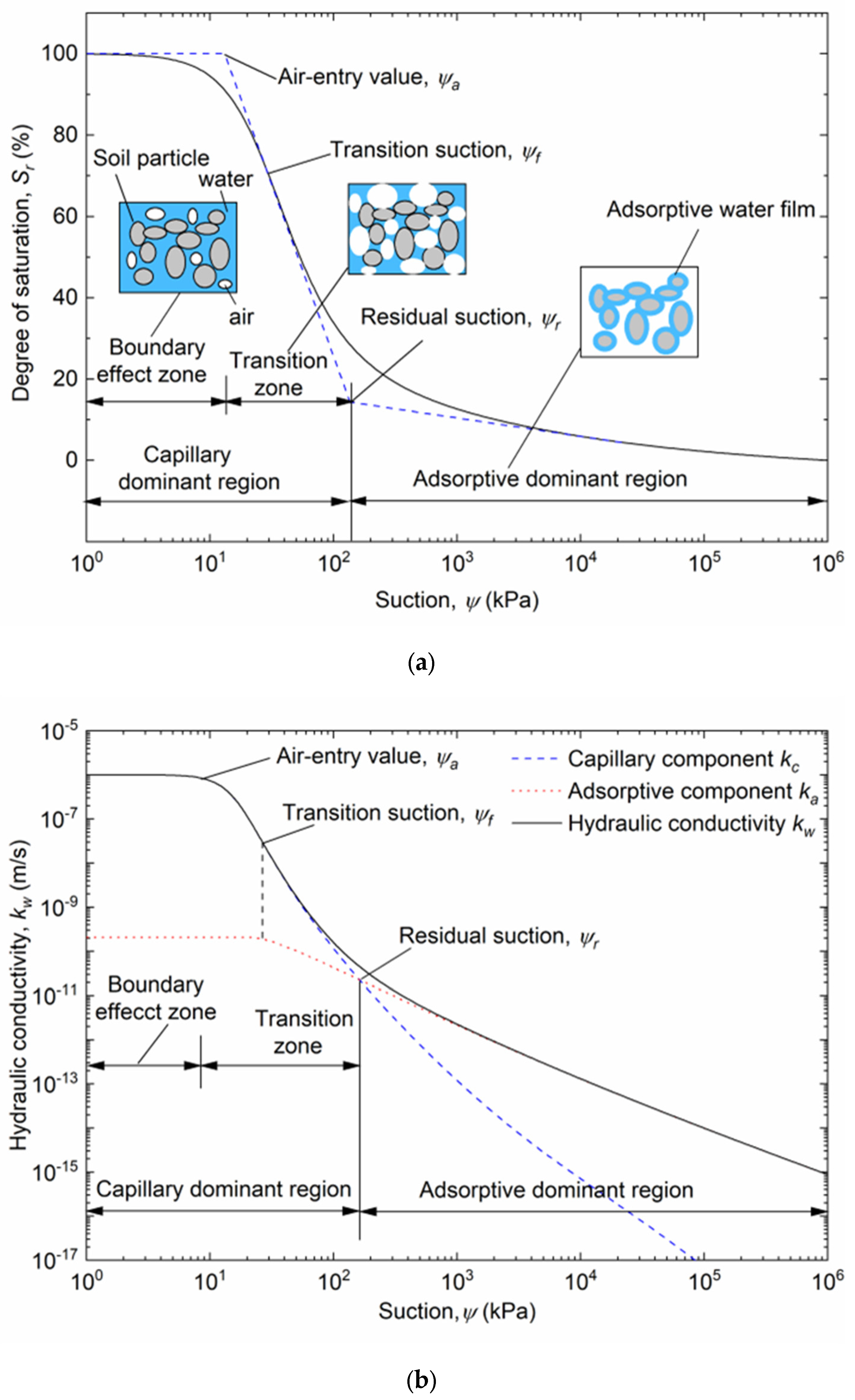
Depending on the different soil–water interaction mechanisms, the soil–water characteristic curve and the hydraulic conductivity curve can be divided into three segments: the boundary effect zone, transition zone and adsorptive dominant region, where the air-entry value and residual suction are two inflection points.

(2)

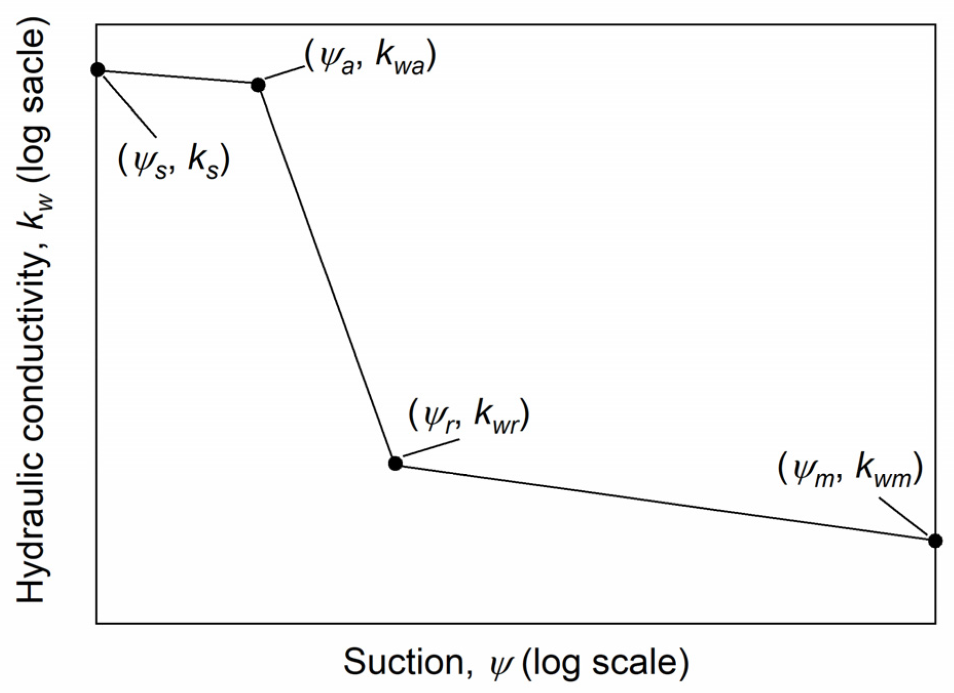
A simple hydraulic conductivity model for unsaturated soil composed of three straight lines has been proposed. Model parameters can be conveniently calibrated by the measured SWCC and the saturated hydraulic conductivity.

(3)

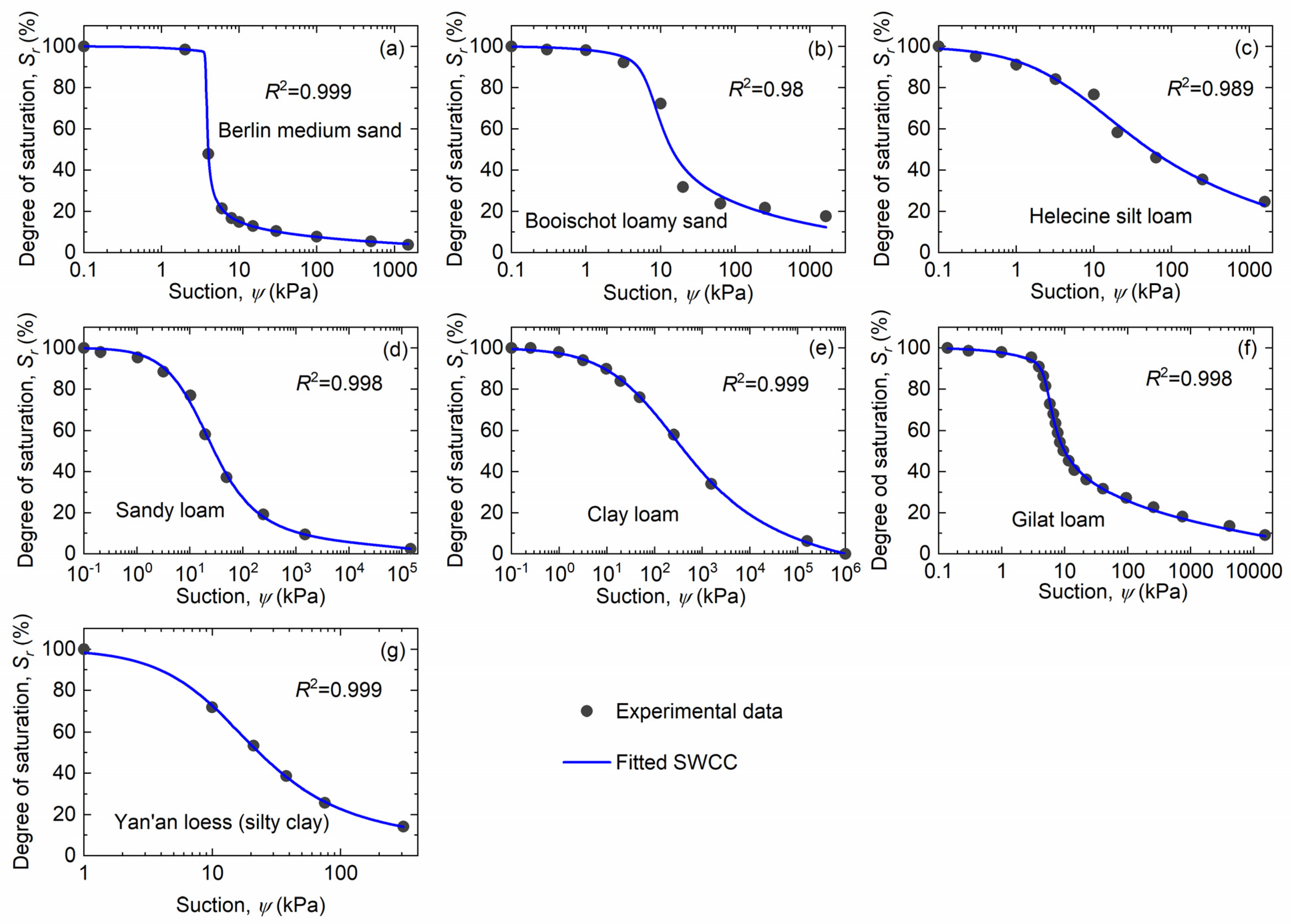
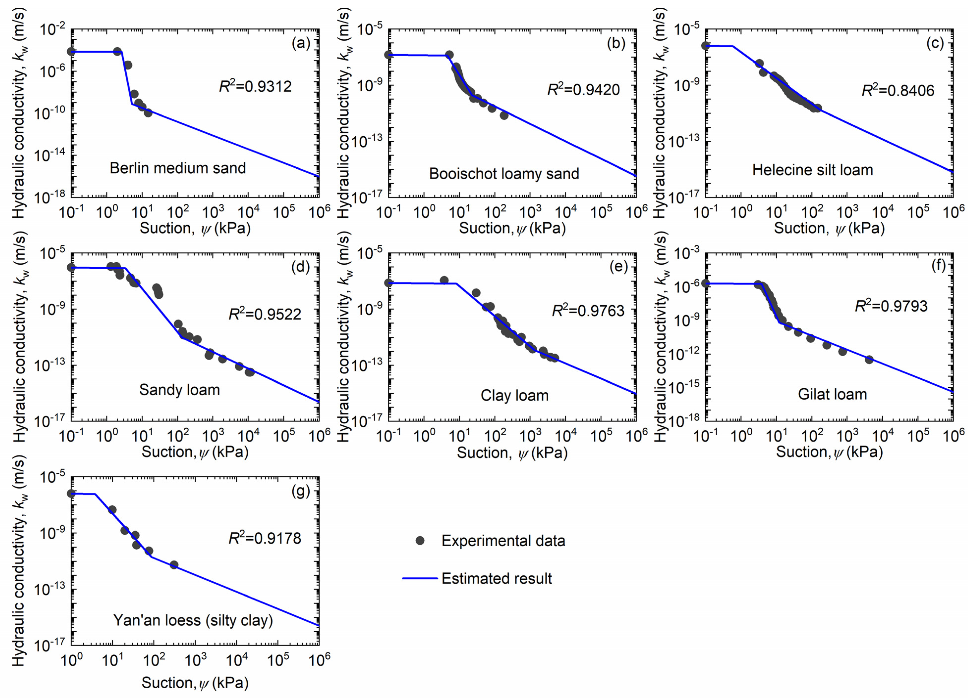
The estimated results, in comparison with the corresponding experimental data, have shown that the proposed model performs well in the estimation of the hydraulic conductivity of different types of soils over a wide suction range.

(4)

Compared with existing approaches, the proposed hydraulic conductivity model has a simple form, and it is unnecessary to calibrate the scaling parameter by the measured unsaturated hydraulic conductivity curve.

References

1. Aleotti, P. A warning system for rainfall-induced shallow failures. Eng. Geol. 2004, 73, 247–265. [Google Scholar] [CrossRef]
2. Le, T.M.H.; Gallipoli, D.; Sanchez, M.; Wheeler, S. Rainfall-induced differential settlements of foundations on heterogeneous unsaturated soils. Géotechnique 2013, 63, 1346–1355. [Google Scholar] [CrossRef]
3. Froude, M.J.; Petley, D.N. Global fatal landslide occurrence from 2004 to 2016. Nat. Hazard Earth Syst. 2018, 18, 2161–2181. [Google Scholar] [CrossRef]
4. Jeong, S.; Kim, Y.; Park, H.; Kim, J. Effects of rainfall infiltration and hysteresis on the settlement of shallow foundations in unsaturated soil. Environ. Earth Sci. 2018, 77, 494. [Google Scholar] [CrossRef]
5. Ng, C.W.W.; Zhou, C.; Chiu, C.F. Constitutive modelling of state-dependent behaviour of unsaturated soils: An overview. Acta Geotech. 2020, 15, 2705–2725. [Google Scholar] [CrossRef]
6. Fredlund, D.G.; Xing, A.Q.; Huang, S.Y. Predicting the permeability function for unsaturated soils using the soil-water characteristic curve. Can. Geotech. J. 1994, 31, 533–546. [Google Scholar] [CrossRef]
7. Tian, K.; Yang, A.; Nie, K.; Zhang, H.; Xu, J.; Wang, X. Experimental study of steady seepage in unsaturated loess soil. Acta Geotech. 2020, 15, 2681–2689. [Google Scholar] [CrossRef]
8. Gallage, C.; Kodikara, J.; Uchimura, T. Laboratory measurement of hydraulic conductivity functions of two unsaturated sandy soils during drying and wetting processes. Soils Found. 2013, 53, 417–430. [Google Scholar] [CrossRef]
9. Leong, E.C.; Rahardjo, H. Permeability functions for unsaturated soils. J. Geotech. Geoenviron. 1997, 123, 1118–1126. [Google Scholar] [CrossRef]
10. Cai, G.; Zhou, A.; Sheng, D. A permeability function for unsaturated soils with different initial densities. Can. Geotech. J. 2014, 51, 1456–1467. [Google Scholar] [CrossRef]
11. Huang, S.Y.; Barbour, S.L.; Fredlund, D.G. Development and verification of a coefficient of permeability function for a deformable unsaturated soil. Can. Geotech. J. 1998, 35, 411–425. [Google Scholar] [CrossRef]
12. Agus, S.S.; Leong, E.C.; Schanz, T. Assessment of statistical models for indirect determination of permeability functions from soil–water characteristic curves. Géotechnique 2003, 53, 279–282. [Google Scholar] [CrossRef]
13. Childs, E.C.; Collis-George, N. The permeability of porous materials. Proc. R. Soc. Lond. 1950, 210, 392–405. [Google Scholar]
14. Marshall, T.J. A relation between permeability and size distribution of pores. J. Soil Sci. 1958, 9, 1–8. [Google Scholar] [CrossRef]
15. Millington, R.J.; Quirk, J.P. Permeability of porous media. Nature 1959, 183, 387–388. [Google Scholar] [CrossRef]
16. Millington, R.J.; Quirk, J.P. Permeability of porous solids. Trans. Faraday Soc. 1961, 57, 1200–1207. [Google Scholar] [CrossRef]
17. Kunze, R.J.; Uehara, G.; Graham, K. Factors Important in the Calculation of Hydraulic Conductivity. Soil Sci. Soc. Am. J. 1968, 32, 760–765. [Google Scholar] [CrossRef]
18. Mualem, Y. A new model for predicting the hydraulic conductivity of unsaturated porous media. Water Resour. Res. 1976, 12, 513–522. [Google Scholar] [CrossRef]
19. Mualem, Y. Hydraulic conductivity of unsaturated porous media: Generalized macroscopic approach. Water Resour. Res. 1978, 14, 325–334. [Google Scholar] [CrossRef]
20. van Genuchten, M.T.H. A closed-form equation for predicting the hydraulic conductivity of unsaturated soils. Soil Sci. Soc. Am. J. 1980, 44, 892–898. [Google Scholar] [CrossRef]
21. Tuller, M.; Or, D. Water films and scaling of soil characteristic curves at low water contents. Water Resour. Res. 2005, 41, W09403. [Google Scholar] [CrossRef]
22. Peters, A.; Durner, W. A simple model for describing hydraulic conductivity in unsaturated porous media accounting for film and capillary flow. Water Resour. Res. 2008, 44, W11417. [Google Scholar] [CrossRef]
23. Tokunaga, T.K. Hydraulic properties of adsorbed water films in unsaturated porous media. Water Resour. Res. 2009, 45, W06415. [Google Scholar] [CrossRef]
24. Tokunaga, T.K. Physicochemical controls on adsorbed water film thickness in unsaturated geological media. Water Resour. Res. 2011, 47, W08514. [Google Scholar] [CrossRef]
25. Lebeau, M.; Konrad, J.M. A new capillary and thin film flow model for predicting the hydraulic conductivity of unsaturated porous media. Water Resour. Res. 2010, 46, W12554. [Google Scholar] [CrossRef]
26. Wang, Y.; Ma, J.; Guan, H. A mathematically continuous model for describing the hydraulic properties of unsaturated porous media over the entire range of matric suctions. J. Hydrol. 2016, 541, 873–888. [Google Scholar] [CrossRef]
27. Wang, Y.; Jin, M.; Deng, Z. Alternative Model for Predicting Soil Hydraulic Conductivity over the Complete Moisture Range. Water Resour. Res. 2018, 54, 6860–6876. [Google Scholar] [CrossRef]
28. Wang, Y.; Ma, R.; Zhu, G. Improved Prediction of Hydraulic Conductivity with a Soil Water Retention Curve That Accounts for Both Capillary and Adsorption Forces. Water Resour. Res. 2022, 58, e2021WR031297. [Google Scholar] [CrossRef]
29. Peters, A. Simple consistent models for water retention and hydraulic conductivity in the complete moisture range. Water Resour. Res. 2013, 49, 6765–6780. [Google Scholar] [CrossRef]
30. Peters, A.; Hohenbrink, T.L.; Iden, S.C.; Durner, W. A Simple Model to Predict Hydraulic Conductivity in Medium to Dry Soil from the Water Retention Curve. Water Resour. Res. 2021, 57, e2020WR029211. [Google Scholar] [CrossRef]
31. Gou, L.; Zhang, C.; Lu, N.; Hu, S. A Soil Hydraulic Conductivity Equation Incorporating Adsorption and Capillarity. J. Geotech. Geoenviron. 2023, 149, 04023056. [Google Scholar] [CrossRef]
32. Corey, A.T.; Brooks, R.H. The Brooks-Corey relationships. In Proceedings of the International Workshop on Characterization and Measurement of the Hydraulic Properties of Unsaturated Porous Media; van Genuchten, M.T., Leij, F.J., Wu, L., Eds.; University of California: Riverside, CA, USA, 1999; pp. 13–18. [Google Scholar]
33. Vanapalli, S.K.; Fredlund, D.G.; Pufahl, D.E. The influence of soil structure and stress history on the soil–water characteristics of a compacted till. Géotechnique 1999, 49, 143–159. [Google Scholar] [CrossRef]
34. Leong, E.C.; Rahardjo, H. Review of soil-water characteristic curve equations. J. Geotech. Geoenviron. 1997, 123, 1106–1117. [Google Scholar] [CrossRef]
35. Fredlund, D.G.; Xing, A.Q. Equations for the soil-water characteristic curve. Can. Geotech. J. 1994, 31, 521–532. [Google Scholar] [CrossRef]
36. Gao, Y.; Sun, D.A. Determination of basic parameters of unimodal and bimodal soil water characteristic curves. Chin. J. Geotech. Eng. 2017, 39, 1884–1891. [Google Scholar]
37. Lu, N.; Zhang, C. Soil sorptive potential: Concept, theory, and verification. J. Geotech. Geoenviron. 2019, 145, 04019006. [Google Scholar] [CrossRef]
38. Chen, K.; Chen, H. Generalized hydraulic conductivity model for capillary and adsorbed film flow. Hydrogeol. J. 2020, 28, 2259–2274. [Google Scholar] [CrossRef]
39. Langmuir, I. Repulsive forces between charged surfaces in water, and the cause of the Jones-ray effect. Science 1938, 88, 430–432. [Google Scholar] [CrossRef]
40. Derjaguin, B.V.; Churaev, N.V.; Muller, V.M. Surface Forces; Plenum: New York, NY, USA, 1987. [Google Scholar]
41. Zhai, Q.; Rahardjo, H. Determination of soil–water characteristic curve variables. Comput. Geotech. 2012, 42, 37–43. [Google Scholar] [CrossRef]
42. Zhai, Q.; Rahardjo, H. Estimation of permeability function from the soil–water characteristic curve. Eng. Geol. 2015, 199, 148–156. [Google Scholar] [CrossRef]
43. Zhang, D. A Coefficient of Determination for Generalized Linear Models. Am. Stat. 2017, 71, 310–316. [Google Scholar] [CrossRef]
44. Nemes, A.D.; Schaap, M.G.; Leij, F.J.; Wösten, J.H.M. Description of the unsaturated soil hydraulic database UNSODA version 2.0. J. Hydrol. 2001, 251, 151–162. [Google Scholar] [CrossRef]
45. Pachepsky, Y.; Scherbakov, R.; Varallyay, G.; Rajkai, K. On obtaining soil hydraulic conductivity curves from water retention curves. Pochvovedenie 1984, 10, 60–72. [Google Scholar]
46. Mualem, Y. A Catalogue of the Hydraulic Properties of Unsaturated Soils; Technical Report; Israel Institute of Technology: Haifa, Israel, 1976. [Google Scholar]
Figure 1. Soil–water interaction mechanisms: (a) soil–water characteristic curve; (b) hydraulic conductivity curve (modifications of [25,31,33]). Parameters Ψa, Ψf and Ψr are the air-entry value, transition suction and residual suction, respectively. Parameter kw is the soil hydraulic conductivity, and parameters kc and ka are the capillary and adsorptive components of the hydraulic conductivity, respectively.
Applsci 14 01254 g001
Figure 2. The proposed simple piecewise model of hydraulic conductivity. Parameters Ψs, Ψa, Ψr and Ψm are the minimum suction, air-entry value, residual suction and highest suction, respectively. ks, kwa, kwr and kwm are the hydraulic conductivities corresponding to the suctions of Ψs, Ψa, Ψr and Ψm, respectively.
Applsci 14 01254 g002
Figure 3. The variation in Πme with the adsorptive water film thickness. The parameters Πm and Πe are the molecular and ionic-electrostatic potentials, respectively.
Applsci 14 01254 g003
Figure 4. Fitted SWCCs for different soils: (a) Berlin medium sand; (b) Booischot loamy sand; (c) Helecine silt loam; (d) Sandy loam; (e) Clay loam; (f) Gilat loam; (g) Yan’an loess (silty clay).
Applsci 14 01254 g004
Figure 5. Estimated hydraulic conductivity functions for the selected soils: (a) Berlin medium sand; (b) Booischot loamy sand; (c) Helecine silt loam; (d) Sandy loam; (e) Clay loam; (f) Gilat loam; (g) Yan’an loess (silty clay).
Applsci 14 01254 g005