Abstract
Recent advancements in crime prediction have increasingly focused on street networks, which offer finer granularity and a closer reflection of real-world urban dynamics. However, existing studies on street-level graph representation learning often overlook the variability in node features when aggregating information from neighboring nodes. This limitation reduces the model’s capacity to fully capture the diverse street attributes and their influence on crime patterns. To address this issue, we introduce an end-to-end deep spatio-temporal learning model that employs a graph attention mechanism (GAT) to analyze the spatio-temporal features of 110 call incidents. Experimental results show that our proposed model outperforms existing methods across multiple prediction metrics. Additionally, ablation studies confirm that the GAT’s capacity to capture spatial dependencies within the street network significantly enhances the model’s overall predictive performance.
1. Introduction
Since its establishment in 1987, the 110 call for police service (hereinafter referred to as “110 Call”) has been responsible for receiving information on potential illegal and criminal incidents. It dispatches the nearest police force to respond to and handle these incidents promptly based on the specific content [1,2]. After nearly four decades of development, the platform has become deeply ingrained in the public consciousness and the most important focus for the local police. Although only a small proportion of the 110 Call incidents are ultimately referred to as crime cases, the local police have to respond to each one of them and dispatch police forces to the scene for handling any issues, thus becoming a core part of the police’s daily work. Due to the continuous and rapid increase in 110 Call incidents in recent years, the existing police force has become overextended, highlighting the urgent need to implement predictive technologies. If it were possible to predict the 110 Call incidents through scientific methods, it could assist the police in better deploying their forces and improving the response efficiency.
By analyzing historical 110 Call records, we find that their underlying principles, particularly in terms of the spatio-temporal distribution characteristics, can be informed by the relevant crime prediction literature. To date, the evolution of crime prediction has advanced from basic analyses to sophisticated deep learning methodologies that integrate crime data with various multimodal sources. The spatial unit has gradually shifted from a grid-based region to a street network, as street networks better reflect real-life scenarios and effectively guide police in timely responses and daily operations [3].
While prior research has produced significant results in terms of crime and traffic analysis at the street level, many studies, such as those by Zhang, Luo, He, Hipp and Deng [4,5,6,7,8], primarily emphasize the impact of built environment factors on crime, overlooking the interrelationships among streets within the network. Others, like Rosser and Zhang [9,10], explore crime diffusion in the street network but neglect the inherent properties of individual streets.
Recent advancements in graph representation learning have treated street networks as graphs, such as the studies by Gu and Yu [11,12], typically assigning equal weights to all the nodes (with streets represented as nodes). This method fails to consider the significant differences in street attributes and spatial structural relationships between nodes. This treatment leads to overlooking variations in the degree of mutual influence between nodes, which can impact the accuracy of the model in capturing the true dynamics of the street network. To solve this problem, we introduce an attention mechanism (graph attention network, GAT) that addresses these differences from the outset, employing stacked GAT layers to automatically learn the varying weights of streets, integrating temporal and external environmental features to improve the prediction outcomes [13].
2. Related Work
2.1. Crime Prediction
The theory of spatial criminology research primarily focuses on two aspects. The first is the theory of criminal opportunities, which examines the factors influencing the spatio-temporal distribution and concentration pattern of crime. The second is social control theory, which explores how structural factors shape neighborhood crime rates by affecting the emergent attributes of the community [3]. Within the realm of opportunity theory, the most well-known frameworks are crime pattern theory [14,15] and routine activity theory [16,17]. These theories conceptualize an urban environment where motivated offenders navigate the area and identify suitable targets in the absence of effective guardians. Specific locations within the built environment are identified as crime attractors and generators, with numerous studies validating these theoretical assumptions. On the other hand, social control theory [18] emphasizes the impact of a region’s socio-economic characteristics, such as the population size, income, education level, and unemployment rate, on crime occurrence.
Early criminological research observed that the occurrence of crime is not randomly distributed across time and space but instead exhibits a pattern of repeat victimization [19]. Consequently, fitting specific regression models to the trends and patterns of crime occurrence became the initial method and means of crime prediction. At this stage, the focus was primarily on the spatio-temporal characteristics of crime incidents, specifically the periodic patterns of their occurrence and the proximity of the locations involved. Bowers et al. proposed the prospective mapping approach to predict and map the future locations of crime [20]. Townsley et al. tested the near repeat hypothesis by using the contagion model [21]. Kalinic et al. applied the kernel density estimation model to detect criminal hotspots [22,23], Mohler et al. implemented the self-exciting point process to model crime [24]. Corcoran et al. introduced the neural network to crime prediction [25].
Subsequent studies revealed that, in addition to the spatio-temporal characteristics of crime incidents, the socio-economic factors of the area and the distribution of the built environment also exhibit a significant correlation with crime. Accordingly, these corresponding indicator features were also incorporated into the crime prediction models to improve the accuracy of the forecasts. Kennedy et al. demonstrated that the risk terrain model can improve crime hotspot mapping [26]. Law et al. explored Bayesian spatio-temporal methods for crime pattern analysis [27]. Bernasco et al. applied the discrete choice framework to analyze burglary location choice [28]. Ge et al. introduced the tensor decomposition method into crime modeling [29]. Wang et al. presented a graph-based deep model to forecast sparse crime [30]. Shiode et al. proposed the flexible search window approach to detect crime hotspots [31].
With the fast development of mobile internet technology, the patterns and characteristics of people’s travel further enriched the scope of opportunity theory research, which helped improve the crime prediction. Through the analysis of human movement patterns, including daily commuting behaviors and the influx of individuals during specific events, researchers seek to enhance their understanding of crime hotspots and trends. Kadar et al. leveraged Foursquare, subway, and taxi data to improve crime prediction [32]. Song et al. conducted a comparative analysis of four indicators associated with theft: the residential, subway, taxi, and mobile phone activity [33]. Song et al. discovered that communities with higher levels of connectivity to the offender’s residence, as indicated by population flow patterns, are more likely to be targeted for theft [34].
Technological advancements, along with data improvements, have significantly advanced crime prediction research. The integration of deep learning models and multi-source data, particularly through graph representation learning, is a key focus. For example, Sun et al. designed CrimeForecaster to capture temporal patterns with gated recurrent networks and cross-region dependencies with diffusion convolution modules [35]. Wang et al. introduced HAGEN, which optimizes region graphs with diffusion convolution [36]. Liang et al. developed the neural attentive framework for hour-level crime prediction (NAHC), using multi-graph convolutional networks to capture spatial dependencies [37]. However, these models are mainly region-based. To enhance the practical results, research needs to move toward more refined, detailed scales.
2.2. Street Network Modeling of Crime
Since the beginning of the 21st century, a growing number of criminologists have shifted their focus to street networks, as this spatial unit more closely aligns with people’s daily lives and travel patterns. Consequently, research on crime prediction based on street networks has gradually become a prominent area of interest. Research on crime within the context of street networks can generally be divided into two main approaches. The first approach focuses on the spatial attributes and socio-economic characteristics of street networks, as well as their correlation with and impact on crime. Early studies suggested that streets offer a more natural and efficient framework for policing activities. For instance, Davies et al. proposed a mathematical modeling method based on street networks for predicting burglaries [38]. Frith et al. demonstrated that street network indicators derived from graph theory play a crucial role in the spatial decision-making of burglars [39]. Summers et al. investigated the influence of the street network’s physical layout on severe outdoor violent crimes, finding that higher degrees of integration and choice are associated with an increased likelihood of crime [40]. Additionally, Kim discovered that structural features rooted in social disorganization and criminal opportunities theories significantly influence crime patterns [41].
Subsequently, scholars began incorporating built environment characteristics into crime research based on street networks, particularly utilizing Google Street View (GSV) to provide extensive, objective data for quantitative analysis. For example, Zeng et al. collected environmental data through field survey and found that the functions of street buildings and the escape paths significantly impact street theft and robbery [42]. Zhang et al. were pioneers in integrating GSV into street-based crime prediction, combining it with data from Twitter and Foursquare to obtain visual, textual, and human activity information, resulting in significant improvements in crime prediction accuracy [4]. Since then, the use of streetscape data has become a prominent area of focus in street-based crime analysis, leading to numerous research developments. For instance, Luo et al. developed a zero-inflated negative binomial regression model to investigate the relationship between different geographic environmental variables and the risk of street crime [5]. He et al. performed a multi-scale analysis to examine how the built environment influences crime occurrence, utilizing data obtained from street view imagery [6]. Hipp et al. extracted 11 features across four dimensions and employed machine learning to demonstrate their influence on five types of crimes [7]. Deng et al. computed eight indicators and employed a Poisson regression model to explore the relationship between streetscape data and crime patterns [8].
The aforementioned research has undoubtedly advanced street-based crime studies to a new level. However, these studies primarily focus on projecting variables such as socio-economic characteristics and built environment attributes onto streets for correlation analysis, with limited attention paid to the topological structure of street networks. Therefore, some researchers have sought to treat the street network as an integrated whole, applying graph theory to analyze and forecast crime by modeling the spatial relationships and interactions within the street network. For example, Rosser et al. introduced the first predictive crime mapping method based on street networks, known as NTKDE. This approach adapted KDE, originally used in prospective mapping, to the network space. It demonstrated superior prediction accuracy for property crime compared to traditional grid-based methods [9]. The development of GLDNet, a deep learning model for network-based predictive mapping, marked a significant advancement over NTKDE. GLDNet utilized a graph-based representation of network-structured data and incorporated a localized diffusion network to effectively model spatial propagation [10].
With the introduction of graph representation learning methods into crime research, it became possible to simultaneously learn street attributes and the structural features of street networks. For instance, Gu et al. applied Deepwalk to derive the topological structure embeddings of a street network called SN2V, and they obtained the embeddings of a heterogeneous information network through link prediction tasks called HIN2V and fed both embeddings into the DeepFM model for street-level crime prediction [11]. A model based on GCN named as DSTGCN was proposed by Yu et al. [12]. The model performs graph convolutional operations on spatial information combined with dynamic variations in temporal and external perspective for traffic accident prediction at the street level. However, such methods generally assign equal weight to all the neighboring nodes without accounting for the varying contributions of different nodes during the aggregation and propagation of information. In practical applications, real-world graphs frequently exhibit noise through the presence of connections between different nodes. This can result in acquiring suboptimal representations due to their failure to distinguish between nodes within neighborhoods [43].
Addressing the biases in crime prediction related to weight allocation within the street network remains a critical challenge. The introduction of graph attention networks (GATs) offers a promising solution, as its self-attention mechanism enables the learning of node features from multiple perspectives, enhancing the richness and robustness of the feature representations [44]. Additionally, the GAT’s ability to dynamically capture the relationships between nodes, rather than relying solely on static graph structures or initial node features, is particularly relevant for real-time incident prediction. These advancements highlight the potential of a GAT to significantly improve predictive accuracy and provide deeper insights into the spatial dynamics of urban crime.
3. Data for Study
The study area for this research is Chaoyang District in Beijing, which is located in the central southern part of the city, covering a total area of 470.8 square kilometers, with 24 sub-districts. In 2019, the permanent population was over 3.47 million people, and the GDP reached more than CNY 711.6 billion, both of which have been consistently ranked at the forefront in Beijing.
The proliferation of open-source resources such as OpenStreetMap (OSM) has greatly improved the accessibility of extensive street network data. In this study, the street network data for Chaoyang District forms the foundational layer for the entire analysis, and 9654 instances of street information are acquired from OSM. These street segments include some basic categorical information, such as the length and type. Figure 1 illustrates the location and street network of Chaoyang District in Beijing.
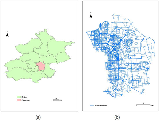
Figure 1.
Map of Chaoyang District: (a) location of Chaoyang District in Beijing; and (b) street network of Chaoyang District.
3.1. 110 Call Records
The data consist of all the 110 Call records in Chaoyang District, Beijing, for the year 2019. Any record lacking essential details like the incident’s address was excluded, as these cannot be accurately used in the research. For repeated alarms, those triggered for the same incident within a short time (typically within tens of minutes) were combined into a single record. After these steps, the dataset was reduced to 377,260 records, which retained 95.2% of the original records. The records encompass various types of incidents, which have been classified into three categories: crime-related (148,208 incidents), security-related (172,087 incidents), and assistance-related (56,965 incidents). The crime-related incidents primarily include personal assault, robbery, theft, and fraud. The security-related incidents encompass economic disputes, neighborhood conflicts, noise complaints, harassment, and traffic accidents. The assistance-related incidents involve situations such as missing persons, lost items and requests for assistance. The main content includes the time of the call and the address. The address information is in the form of the latitude and longitude. A distance-based mapping algorithm was employed to calculate the Euclidean distance between each incident location and the nearest street segment. The nearest neighbor analysis tool in ArcGIS 10.6 was used to match each incident to its closest street. To ensure accuracy, we adhered to geocoding standards, achieving a hit rate above the 85% reliability threshold recommended by Ratcliffe [45]. The distribution of all the incidents across the street network is depicted in Figure 2.
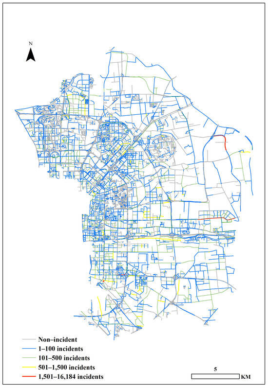
Figure 2.
Distribution of 110 Call incidents in 2019 across the street network. The five colors in the figure represent the cumulative number of incidents on the street throughout the year, with the following breakdown: gray indicates no incidents, blue represents 1–100 incidents, green represents 101–500 incidents, yellow represents 501–1500 incidents, and red represents over 1500 incidents.
3.2. Population
The population data utilized in this article are obtained from the WorldPop website, with a spatial resolution of 100 m. Given the raster-based nature of these data, preprocessing is necessary to accurately align the data with the street network. In ArcGIS, the Chaoyang District is divided into a grid of 100 m × 100 m cells, corresponding to the population data provided by WorldPop. All the streets obtained from OSM intersect with these grid cells, resulting in the division of streets into multiple segments at the intersection points. Within each grid cell, the population is proportionally distributed among the street segments based on their length. The population count for each street segment is thereby determined within the corresponding grid cell. Subsequently, the total population for each street is calculated by summing the population counts of all its segments. Figure 3 depicts the spatial distribution of the population throughout the street network.
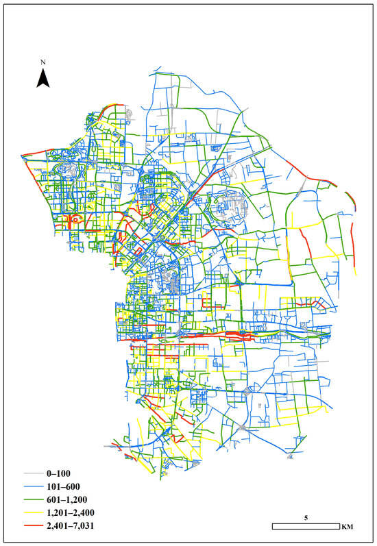
Figure 3.
Spatial distribution of the population throughout the street network.
3.3. POIs
Points of interest (POIs) are utilized to characterize the land use features of particular locations. The dataset, which includes 14 categories, such as dining, scenery, and facilities, was sourced from the API offered by Baidu Map Service. As these data are geospatial, consisting of latitude and longitude coordinates, they can be associated with street segments by calculating the nearest neighbor. A total of 138,356 POIs were downloaded for analysis. Figure 4 presents the spatial distribution of the POIs throughout the street network.
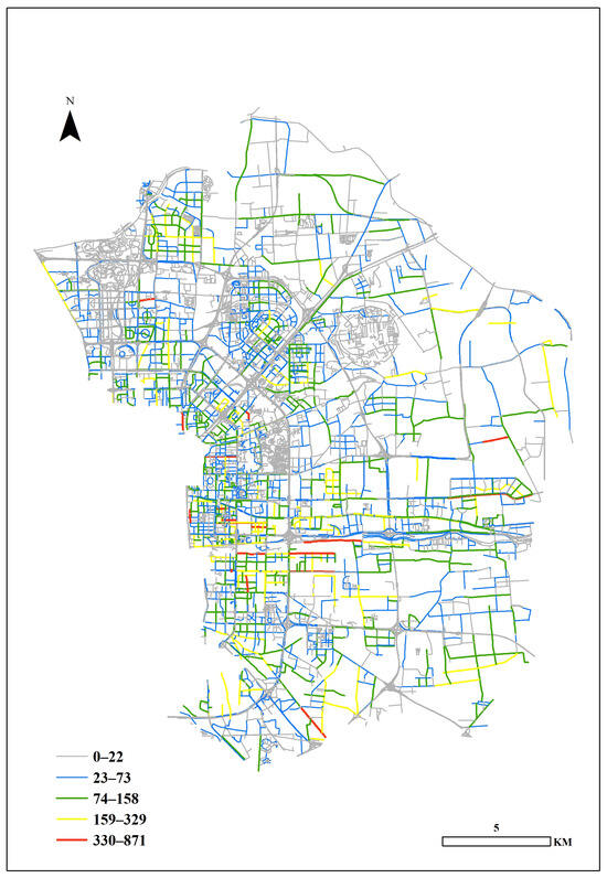
Figure 4.
Spatial distribution of the POIs throughout the street network.
3.4. Meteorological Data
The weather data used in this study were obtained from a meteorological monitoring station located within the study area, covering the entire year of 2019, with hourly granularity. This dataset includes variables such as the wind speed, temperature, atmospheric pressure, humidity, and precipitation, among others.
A comprehensive summary of all the spatio-temporal features is presented in Table 1.

Table 1.
Spatio-temporal features list.
4. Problem Statement
The aim of this study is to forecast the probability of 110 Call incidents for each street over the subsequent hour. The features input into the forecasting model are primarily categorized into spatial features based on the graph structure, temporal features based on the calendar information, and external environmental features based on the weather information. This study adopts different feature representation methods according to the characteristics of these three types of features to obtain embedded vectors, which are ultimately used for discrimination by a binary classifier. In this section, we begin by presenting the representation learning methods applied to the three types of features, followed by a comprehensive description of the overall model architecture.
4.1. Graph Representation
Consider a graph G = (V, E, X, A), where V represents the nodes in the graph, E represents the edges connecting the nodes, X denotes the node features, and A is the adjacency matrix. An adjacency matrix is a mathematical representation of a graph where each row and column corresponds to a node (or street), and the entries indicate whether pairs of nodes are adjacent (connected) in the graph. In our study, the adjacency matrix represents the connectivity between street segments in the urban road network. If Aij = 1, nodes vi and vj are adjacent; otherwise, they are not. When applying graph methods to represent street networks, two common approaches are often used.
The first is the primary graph, where V represents intersections and E represents the streets connecting them. This method is advantageous as it accounts for the heterogeneous characteristics of both intersections and streets.
The second approach is the dual graph [46], which is the inverse of the primary graph: V represents streets, and E represents the intersections connecting those streets. A dual graph is a graph that represents the relationships between the edges (streets) of the original graph rather than the nodes (intersections). In this context, each node in the dual graph corresponds to a street segment, and the edges between the nodes represent the adjacency, or connectivity, between street segments. This method emphasizes the properties of the streets and the topological features of the entire network, aligning more closely with the objectives of our research. Consequently, we opted for the dual graph approach.
Figure 5 illustrates the operational process of this method: panel (a) shows a simplified real-world street network, while panel (b) displays the transformed network produced by this approach. In the transformed network, the red node v6 represents the target street, with the adjacent nodes corresponding to neighboring streets, numbered 2, 3, 8, and 9, respectively.
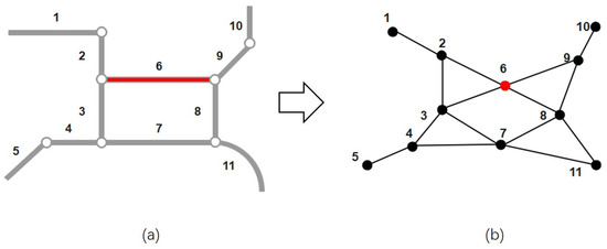
Figure 5.
Operational process of the dual graph method: (a) a simplified real-world street network, the numbers represent street segment identifiers; and (b) the transformed network, the numbers next to the nodes correspond to the street segments in Figure (a).
Accordingly, utilizing the dual graph method, we constructed a graph G = (V, X, A), where V denotes all the streets within our study area. X ∈ R|V|×M encapsulates the spatial features of these streets, with |V| = 9654 and M = 36. A is the adjacency matrix of the streets, indicating whether a pair of nodes (streets) intersect with one another.
4.2. Spatial Embedding
A GAT is a type of graph neural network that incorporates the attention mechanism. This allows the GAT to simultaneously capture both node features and topological structure features, while also differentiating the importance of various neighboring nodes. This approach addresses a key limitation of GCNs, which treat all the neighboring nodes as having equal importance [47]. The working principle of the GAT involves several key steps: feature aggregation with attention, attention coefficients calculation, feature update and multi-head attention.
At first, the GAT utilizes a single-layer feedforward neural network as its alignment mechanism to determine the attention scores between node pairs. This approach allows for the calculation of the relative importance of the connections between the nodes in the graph.
where and indicate the hidden representations of the node and in the layer, is the neighbor of , represents the operation of concatenation, is a learnable weight, denotes the transposition operation, and LeakyReLU is a non-linear activation function.
In this step, the GAT restricts its computation to masked attention, focusing solely on each node’s immediate, first-order neighbors through the use of localized attention mechanisms. Then, the GAT uses the following equation to normalize the attention scores:
where and are the neighboring nodes of node .
After obtaining the normalized attention coefficients , these values are utilized to compute a weighted linear combination of the associated features. This combined result is then passed through a non-linear activation function , producing the final output features:
To enhance the stability of the learning process, a multi-head attention mechanism can be incorporated, building upon the self-attention process. In this approach, independent attention mechanisms are applied to perform the transformation described in Equation (3). The resulting features from each attention head are then concatenated to produce the final output feature representation.
where || represents the concatenation, represents the normalized attention coefficient generated by the k-th attention mechanism , and denotes the corresponding weight matrix.
Upon completing the sequence of operations outlined, the GAT produces the final output, which is the embedding representation of a given node within the overall graph structure. The embedding encapsulates not only the spatial attributes of the node but also the impact of its neighboring nodes. It integrates information derived from the graph’s overall structure and the features of adjacent nodes, providing a comprehensive representation.
4.3. Temporal Embedding
In this study, the selected temporal features are primarily derived from calendar attributes. To extract features from this type of data, the model utilizes a stacked multi-layer neural network, which is well suited for capturing complex patterns and relationships within the temporal features.
4.4. External Embedding
The external features primarily originate from the weather data, which are recorded with hourly precision, aligning with the granularity of the 110 Call incident risk predictions. To thoroughly explore the hidden correlation between these features and the prediction target, we have employed the long short-term memory (LSTM) model [48]. The LSTM component is adept at capturing temporal dependencies and variations in the weather data over specific time periods, thereby advancing the model’s ability to predict the incident risk.
4.5. Model Architecture
The training data comprise quadruples (xspa, xtem, xext, y), where xspa, xtem, and xext denote spatio-temporal features potentially associated with incident occurrence, and y indicates whether an incident has occurred in a specific street segment. Specifically, xspa represents the street network embedding, xspa corresponds to the temporal embedding, and xext denotes the external environment embedding. Consequently, the prediction task is effectively framed as a binary classification problem, as illustrated in Figure 6.
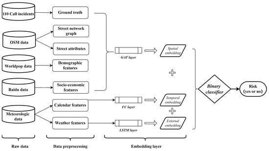
Figure 6.
DSTGAT architecture.
5. Experiment
We carried out a series of experiments and benchmarked our proposed model against several established deep learning models from prior research to assess its effectiveness. Following this, we conducted ablation studies to evaluate the impact of various features or components on the predictive performance.
5.1. Hardware and Software Conditions
The Inspur (Beijing, China) server used for the experiment is equipped with a 32-core CPU, 128 GB of memory, and dual A100 GPUs, and the operating system is Ubuntu 20.04.
5.2. Dataset Preparation
In practical applications, although historical 110 Call incidents data are more abundant than crime data, these data remain sparse. To mitigate the potential negative effects of imbalanced datasets on the model, it is crucial to appropriately balance the training data. Undersampling was used to balance the dataset, focusing the model on incident records without being overwhelmed by the large number of non-incident samples. This approach avoids the increased computational complexity and resource demands of oversampling techniques, while stratified sampling was employed to minimize the information loss by maintaining a representative distribution of non-incident data across locations and times. Both types of samples were then combined to create a balanced dataset. The dataset was shuffled to remove any bias before being split into training (60%), validation (20%), and testing (20%) subsets. Stratified sampling was used to maintain proportional representation of categories across all the subsets and to account for the dataset’s hourly temporal characteristics. Multiple rounds of partitioning ensured consistent results and minimized any single partition’s influence on the model performance.
5.3. Evaluation Metrics
In this article, we approach 110 Call incident risk prediction as a binary classification problem. Consequently, we utilize four standard evaluation metrics pertinent to classification tasks: accuracy (ACC), F1-score, area under the curve (AUC), and root mean squared error (RMSE).
ACC is a fundamental evaluation metric used to measure the proportion of correctly classified instances among the total number of instances. ACC provides a straightforward indication of the overall performance of a classification model. It is defined as:
The F1-score is a metric that combines both precision and recall into a single measure, providing a balance between them. It is defined as the harmonic mean of the precision (the proportion of true positive predictions among all the positive predictions) and recall (the proportion of true positive predictions among all the actual positives). It is calculated as:
The AUC refers to the area under the receiver operating characteristic (ROC) curve. The AUC quantifies the overall ability of the model to discriminate between positive and negative classes, with values ranging from 0 to 1. An AUC of 1 indicates perfect classification, while an AUC of 0.5 suggests no discrimination ability.
The RMSE is a widely used metric for assessing the regression accuracy of prediction models. It measures the average magnitude of the prediction errors, giving an indication of how well the model predicts continuous outcomes. The RMSE is defined as:
5.4. Baseline Models
The baseline models included traditional machine learning models (Random Forest [49], XGBoost [50]) and deep learning models (DeepFM [51], AFM [52], DCN [53], NFM [54]), along with a street-level prediction model (DSTGCN [12] based on graph convolution).
To optimize the traditional models, a grid search was used with the following parameter ranges. Random Forest: n_estimators = [100, 200], max_depth = [None, 10, 20], class_weight = [“balanced”]; XGBoost: n_estimators = [100, 200], learning_rate = [0.01, 0.1], max_depth = [3, 5, 7].
The hyperparameter settings for the deep learning models were as follows. AFM: attention_factor = 8, l2_reg_linear = 1 × 10⁻⁵, l2_reg_embedding = 1 × 10⁻⁵; DCN: dnn_hidden_units = (256, 128, 64), dnn_dropout = 0.5, l2_reg_embedding = 1 × 10⁻⁴; NFM: dnn_hidden_units = (256, 128, 64), dnn_dropout = 0.5, l2_reg_embedding = 1 × 10⁻⁴; DeepFM: dnn_hidden_units = (256, 128, 64), dnn_dropout = 0.5, l2_reg_embedding = 1 × 10⁻⁴. The batch size for the aforementioned models was set in the range of {32, 64, 128, 256, 512}, with 64 yielding the best results after experimental comparison. The optimizer used for the models was Adam, and the loss function was binary_crossentropy.
The hyperparameter settings for DSTGCN and our model DSTGAT were as follows: optimizer = Adam, loss function = binary_crossentropy, learning rate = 0.001, weight decay = 0.001, hop = {1, 2, 3, 4} with 2 yielding the best result, batch size = {64, 128, 256, 512} with 512 yielding the best result.
5.5. Experimental Results
Table 2 presents the results of the various models, highlighting the highest-performing model in bold and the second highest in underline.
Table 2.
Experimental results for the 110 Call incidents.
As shown in Table 2 and Figure 7, our study yields several key findings. The models based on GNNs outperform the others, followed by deep learning models and then traditional machine learning models, reflecting technological advancements. On the general test metrics, the traditional machine learning and deep learning models show similar performance, with deep learning being slightly ahead. However, for the specific incident types, the gap widens, with the traditional models, particularly XGBoost, showing more performance fluctuations. The GNN-based models maintain stable, superior performance across all the incident types compared to the other baseline models.
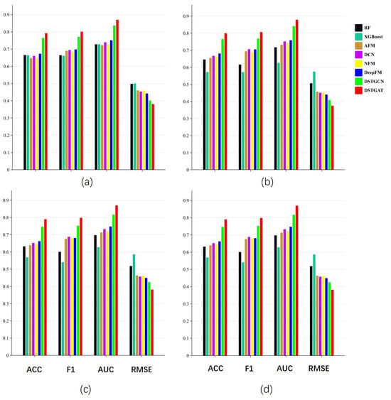
Figure 7.
Result comparison for the 110 Call incidents: (a) all incidents; (b) crime-related incidents; (c) security-related incidents; and (d) assistance-related incidents.
Despite these efforts, the experimental results indicate that even the best-performing model in the deep learning group, DeepFM, falls short when compared to the second group of models based on graph neural networks (GNNs). Specifically, for all the incidents, the DSTGCN model surpasses DeepFM by 15.31%, 12.16%, and 12.94% in terms of the ACC, F1-score, and AUC, respectively, while achieving an 11.27% reduction in the RMSE. Our proposed model, DSTGAT, demonstrates superior performance for all the incidents, exceeding DeepFM by 19.49%, 16.43%, and 17.41% in the ACC, F1, and AUC, respectively, and achieving a 15.76% reduction in the RMSE. These findings corroborate prior research, which has established that the topological structural features of street networks significantly enhance the accuracy of spatio-temporal event prediction tasks [55,56,57].
When comparing the two GNN algorithms, the GAT approach employed in this study has demonstrated superior performance over the GCN method when using the existing spatio-temporal features associated with the 110 Call incidents. Specifically, for all the incidents, DSTGAT surpasses DSTGCN by 3.62%, 3.81%, and 3.96% in the ACC, F1-score, and AUC, respectively, while achieving a 5.06% reduction in the RMSE. Although the improvement over DeepFM is more pronounced, the GAT method consistently outperforms the GCN across all the evaluated metrics for all the three types of 110 Call incidents. This finding suggests that in event prediction tasks based on the graph structure of street networks, the introduction of an attention mechanism effectively mitigates the limitation of GCNs, which treat all the neighboring nodes equally.
A noteworthy finding is that among the three different types of 110 Call incidents, crime-related incidents consistently demonstrated a predictive advantage across all six models tested in the experiments. This was followed by security-related incidents, and lastly, by assistance-related incidents. The comparison of the results for different types of incidents in DSTGAT is illustrated in Figure 8. Consequently, the inclusion of the latter two types can be regarded as introducing a degree of noise, leading to reduced predictive performance for all the incidents when compared to crime-related incidents. This observation also indirectly supports the validity of the criminological theories employed, highlighting their effectiveness in guiding the analysis and prediction of crime occurrence by considering the crime-related spatio-temporal characteristics.
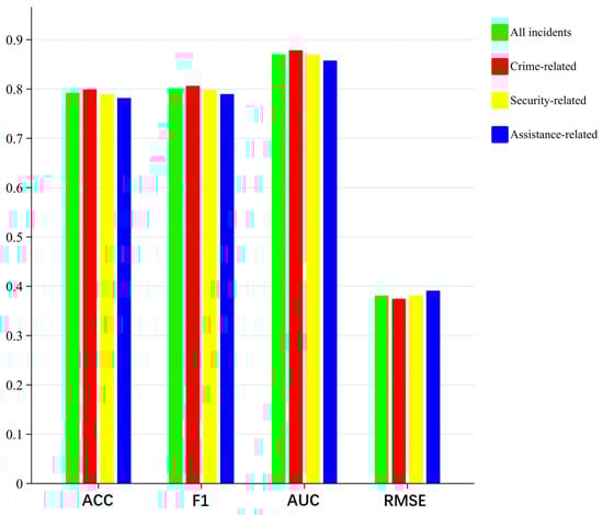
Figure 8.
Result comparison for the different types of incidents in DSTGAT.
5.6. Ablation Experiment
Building upon our foundational experiments, we performed ablation studies to rigorously assess the impact of various features on the model’s predictive capabilities. This study integrates three primary feature representations. Spatial embeddings include the fundamental street characteristics, demographic data, socio-economic indicators (such as points of interest), and the topological structural features of the street network. Temporal embeddings capture the calendar-related features. External embeddings account for the weather conditions. Theoretically, the spatial embeddings are hypothesized to be the most critical, significantly influencing the accuracy of the prediction results.
Specifically, we conducted four sequential ablation studies based on the existing DSTGAT model: first, by removing time-related features and components; second, by removing weather-related features and components; third, by removing both temporal and weather-related features and components; and finally, by removing spatial features and components. By analyzing the experimental results from each ablation study, we can evaluate the impact of each feature and component on the overall model performance.
According to Table 3 and Figure 9, the ablation experiments reveal that the three embeddings we introduced have collectively enhanced the predictive performance. Although end-to-end deep learning models have inherently complex internal structures, making it challenging to isolate the specific contributions of each feature type, ablation studies provide a practical approach to evaluating their relative impact. The results clearly demonstrate that spatial features and components have the most substantial influence on the DSTGAT model.
Table 3.
Results of the ablation experiment.
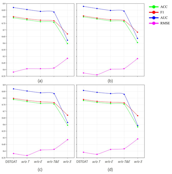
Figure 9.
Ablation experiment result comparison for the 110 Call incidents: (a) all incidents; (b) crime-related incidents; (c) security-related incidents; and (d) assistance-related incidents.
Specifically, using the ablation experiment on the crime-related incidents with the best predictive performance as an example, when only the temporal features were removed, the model’s ACC, F1-score, and AUC decreased by 1.96%, 2.02%, and 1.83%, respectively, while the RMSE increased by 3.76%. When only the external features were removed, the model’s ACC, F1-score, and AUC decreased by 3.84%, 3.56%, and 3.51%, respectively, while the RMSE increased by 7.26%. It can be observed that, in our model, the weather features contribute more significantly to the prediction compared to the features provided by calendar information. The removal of both temporal and weather-related features resulted in not greater changes, with the ACC, F1, and AUC decreasing by only 4.53%, 4.19%, and 4.06%, respectively, and the RMSE increasing by 8.57%.
In contrast, when spatial features were removed, the model’s ACC, F1-score, and AUC decreased by 24.34%, 15.29%, and 27.57%, respectively, while the RMSE increased by 28.96%. These findings underscore the effectiveness of using a GAT-based graph representation method for predicting events within street networks.
6. Conclusions
This study presents a deep spatio-temporal model leveraging the graph attention network (GAT) within a graph neural network framework to predict the likelihood of future 110 Call incidents in specific street segments. The model is designed to extract pertinent features from a diverse set of spatio-temporal data, including the street networks, population density, points of interest (POIs), and calendar and weather conditions. The architecture of the model comprises three primary components, each dedicated to learning spatial, temporal, and external environmental features relevant to the street segments. Empirical evaluations using real-world data underscore the model’s efficacy. We envision integrating our model into an interactive dashboard that law enforcement can use to visualize high-risk streets in real time, with color-coded alerts highlighting incident probabilities. This tool would allow officers to monitor evolving risk patterns across the street network, enabling dynamic resource allocation based on both real-time data and historical trends. Leveraging the GAT’s multi-head attention mechanism, the model identifies and prioritizes critical streets, supporting more targeted and efficient patrol strategies.
The factors contributing to incidents’ risk are highly complex, encompassing not only criminal activities that threaten personal and property security but also historical conflicts between neighbors, among other issues. Consequently, future research should integrate the professional expertise of law enforcement to refine the incident classification, thereby enabling more precise and effective responses by the police.
Author Contributions
Methodology, J.S.; Software, H.G.; Validation, P.C.; Data curation, H.G.; Writing—original draft, J.S.; Supervision, P.C.; Funding acquisition, J.S.; J.S., Ph. D candidate at PPSUC; P.C., Professor at PPSUC; H.G., Ph. D candidate at PPSUC. All authors have read and agreed to the published version of the manuscript.
Funding
This study was funded by the “Double First-Class” innovative research project in criminology at the People’s Public Security University of China (2023SYL03).
Data Availability Statement
The datasets, models, and codes that underpin the conclusions drawn in this research are accessible upon request to the corresponding author, subject to reasonable conditions. Due to privacy concerns, these data are not available for public access.
Acknowledgments
We thank the Beijing Municipal Public Security Bureau for authorizing us to use their data for this research. We also thank anonymous reviewers for their comments on improving this manuscript.
Conflicts of Interest
The authors declare no conflicts of interest.
Appendix A
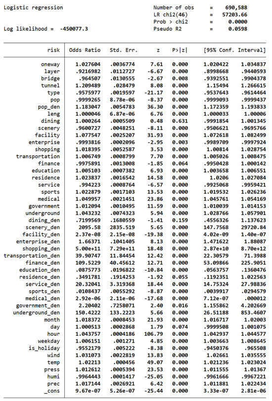
Figure A1.
Logistic regression test result.
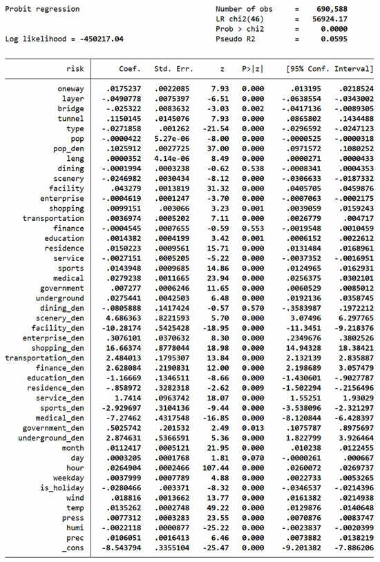
Figure A2.
Probabilistic regression test result.
References
- Wong, K.C. Policing in the People’s Republic of China. The Road to Reform in the 1990s. Br. J. Criminol. 2002, 42, 281–316. [Google Scholar] [CrossRef]
- Dai, M.; Xia, Y.; Han, R. Temporal Variations in Calls for Police Service During COVID-19: Evidence from China. Crime Delinq. 2022, 68, 1183–1206. [Google Scholar] [CrossRef]
- Hipp, J.R.; Williams, S.A. Advances in Spatial Criminology: The Spatial Scale of Crime. Annu. Rev. Criminol. 2020, 3, 75–95. [Google Scholar] [CrossRef]
- Zhang, Y.; Siriaraya, P.; Kawai, Y.; Jatowt, A. Analysis of Street Crime Predictors in Web Open Data. J. Intell. Inf. Syst. 2020, 55, 535–559. [Google Scholar] [CrossRef]
- Luo, L.; Deng, M.; Shi, Y.; Gao, S.; Liu, B. Associating Street Crime Incidences with Geographical Environment in Space Using a Zero-Inflated Negative Binomial Regression Model. Cities 2022, 129, 103834. [Google Scholar] [CrossRef]
- He, Z.; Wang, Z.; Xie, Z.; Wu, L.; Chen, Z. Multiscale Analysis of the Influence of Street Built Environment on Crime Oc-currence Using Street-View Images. Comput. Environ. Urban Syst. 2022, 97, 101865. [Google Scholar] [CrossRef]
- Hipp, J.R.; Lee, S.; Ki, D.; Kim, J.H. Measuring the Built Environment with Google Street View and Machine Learning: Consequences for Crime on Street Segments. J. Quant. Criminol. 2022, 38, 537–565. [Google Scholar] [CrossRef]
- Deng, M.; Yang, W.; Chen, C.; Liu, C. Exploring Associations between Streetscape Factors and Crime Behaviors Using Google Street View Images. Front. Comput. Sci. 2022, 16, 164316. [Google Scholar] [CrossRef]
- Rosser, G.; Davies, T.; Bowers, K.J.; Johnson, S.D.; Cheng, T. Predictive Crime Mapping: Arbitrary Grids or Street Networks? J. Quant. Criminol. 2017, 33, 569–594. [Google Scholar] [CrossRef]
- Zhang, Y.; Cheng, T. Graph Deep Learning Model for Network-Based Predictive Hotspot Mapping of Sparse Spatio-Temporal Events. Comput. Environ. Urban Syst. 2020, 79, 101403. [Google Scholar] [CrossRef]
- Gu, H.; Sui, J.; Chen, P. Graph Representation Learning for Street-Level Crime Prediction. ISPRS Int. J. Geo-Inf. 2024, 13, 229. [Google Scholar] [CrossRef]
- Yu, L.; Du, B.; Hu, X.; Sun, L.; Han, L.; Lv, W. Deep Spatio-Temporal Graph Convolutional Network for Traffic Accident Prediction. Neurocomputing 2021, 423, 135–147. [Google Scholar] [CrossRef]
- Veličković, P.; Cucurull, G.; Casanova, A.; Romero, A.; Liò, P.; Bengio, Y. Graph Attention Networks. arXiv 2018, arXiv:1710.10903. [Google Scholar]
- Brantingham, P.B. Nodes, Paths and Edges: Considerations on the Complexity of Crime and the Physical Environment. J. Environ. Psychol. 1993, 13, 3–28. [Google Scholar] [CrossRef]
- Brantingham, P.; Brantingham, P. Criminality of Place: Crime Generators and Crime Attractors. Eur. J. Crim. Policy Res. 1995, 3, 5–26. [Google Scholar] [CrossRef]
- Cohen, L.E.; Felson, M. Social Change and Crime Rate Trends: A Routine Activity Approach. Am. Sociol. Rev. 1979, 44, 588. [Google Scholar] [CrossRef]
- Sherman, L.W.; Gartin, P.R.; Buerger, M.E. Hot Spots of Predatory Crime: Routine Activities and the Criminology of Place. Criminology 1989, 27, 27–56. [Google Scholar] [CrossRef]
- Sampson, R.J.; Groves, W.B. Community Structure and Crime: Testing Social-Disorganization Theory. Am. J. Sociol. 1989, 94, 774–802. [Google Scholar] [CrossRef]
- Farrell, G.; Pease, K. Once Bitten, Twice Bitten: Repeat Victimisation and Its Implications for Crime Prevention; Police Research Group Crime Prevention Unit Paper: London, UK, 1993. [Google Scholar]
- Bowers, K.J. Prospective Hot-Spotting: The Future of Crime Mapping? Br. J. Criminol. 2004, 44, 641–658. [Google Scholar] [CrossRef]
- Townsley, M.K.; Homel, R.; Chaseling, J. Infectious Burglaries. A Test of the Near Repeat Hypothesis. Br. J. Criminol. 2003, 43, 615–633. [Google Scholar] [CrossRef]
- Chainey, S.; Ratcliffe, J. Identifying Crime Hotspots; John Wiley & Sons, Inc.: Hoboken, NJ, USA, 2013. [Google Scholar]
- Kalinic, M.; Krisp, J.M. Kernel Density Estimation (KDE) vs. Hot-Spot Analysis–Detecting Criminal Hot Spots in the City of San Francisco. In Proceedings of the 21st AGILE Conference on Geographic Information Science, Lund, Sweden, 12–15 June 2018.
- Mohler, G.O.; Short, M.B.; Brantingham, P.J.; Schoenberg, F.P.; Tita, G.E. Self-Exciting Point Process Modeling of Crime. J. Am. Stat. Assoc. 2011, 106, 100–108. [Google Scholar] [CrossRef]
- Corcoran, J.J.; Wilson, I.D.; Ware, J.A. Predicting the Geo-Temporal Variations of Crime and Disorder. Int. J. Forecast. 2003, 19, 623–634. [Google Scholar] [CrossRef]
- Kennedy, L.W.; Caplan, J.M.; Piza, E. Risk Clusters, Hotspots, and Spatial Intelligence: Risk Terrain Modeling as an Algorithm for Police Resource Allocation Strategies. J. Quant. Criminol. 2011, 27, 339–362. [Google Scholar] [CrossRef]
- Law, J.; Quick, M.; Chan, P. Bayesian Spatio-Temporal Modeling for Analysing Local Patterns of Crime Over Time at the Small-Area Level. J. Quant. Criminol. 2014, 30, 57–78. [Google Scholar] [CrossRef]
- Bernasco, W. Modeling Micro-Level Crime Location Choice: Application of the Discrete Choice Framework to Crime at Places. J. Quant. Criminol. 2010, 26, 113–138. [Google Scholar] [CrossRef]
- Ge, L.; Liu, J.; Zhou, A.; Li, H. Crime Rate Inference Using Tensor Decomposition. In Proceedings of the 2018 IEEE SmartWorld, Ubiquitous Intelligence & Computing, Advanced & Trusted Computing, Scalable Computing & Communications, Cloud & Big Data Computing, Internet of People and Smart City Innovation (SmartWorld/SCALCOM/UIC/ATC/CBDCom/IOP/SCI), Guangzhou, China, 8–12 October 2018; IEEE: Guangzhou, China, 2018; pp. 713–717. [Google Scholar]
- Wang, B.; Luo, X.; Zhang, F.; Yuan, B.; Bertozzi, A.L.; Brantingham, P.J. Graph-Based Deep Modeling and Real Time Forecasting of Sparse Spatio-Temporal Data. arXiv 2018, arXiv:1804.00684. [Google Scholar]
- Shiode, S.; Shiode, N. A Network-Based Scan Statistic for Detecting the Exact Location and Extent of Hotspots along Urban Streets. Comput. Environ. Urban Syst. 2020, 83, 101500. [Google Scholar] [CrossRef]
- Kadar, C.; Pletikosa, I. Mining Large-Scale Human Mobility Data for Long-Term Crime Prediction. EPJ Data Sci. 2018, 7, 26. [Google Scholar] [CrossRef]
- Song, G.; Liu, L.; Bernasco, W.; Xiao, L.; Zhou, S.; Liao, W. Testing Indicators of Risk Populations for Theft from the Person across Space and Time: The Significance of Mobility and Outdoor Activity. Ann. Am. Assoc. Geogr. 2018, 108, 1370–1388. [Google Scholar] [CrossRef]
- Song, G.; Bernasco, W.; Liu, L.; Xiao, L.; Zhou, S.; Liao, W. Crime Feeds on Legal Activities: Daily Mobility Flows Help to Explain Thieves’ Target Location Choices. J. Quant. Criminol. 2019, 35, 831–854. [Google Scholar] [CrossRef]
- Sun, J.; Yue, M.; Lin, Z.; Yang, X.; Nocera, L.; Kahn, G.; Shahabi, C. CrimeForecaster: Crime Prediction by Exploiting the Geographical Neighborhoods’ Spatiotemporal Dependencies. In Machine Learning and Knowledge Discovery in Databases. Applied Data Science and Demo Track; Dong, Y., Ifrim, G., Mladenić, D., Saunders, C., Van Hoecke, S., Eds.; ECML PKDD 2020. Lecture Notes in Computer Science; Springer: Cham, Switzerland, 2021; Volume 12461. [Google Scholar] [CrossRef]
- Wang, C.; Lin, Z.; Yang, X.; Sun, J.; Yue, M.; Shahabi, C. HAGEN: Homophily-Aware Graph Convolutional Recurrent Network for Crime Forecasting. In Proceedings of the AAAI Conference on Artificial Intelligence, Online, 22 February–1 March 2022. [Google Scholar]
- Liang, W.; Wang, Y.; Tao, H.; Cao, J. Towards Hour-Level Crime Prediction: A Neural Attentive Framework with Spatial–Temporal-Categorical Fusion. Neurocomputing 2022, 486, 286–297. [Google Scholar] [CrossRef]
- Davies, T.P.; Bishop, S.R. Modelling Patterns of Burglary on Street Networks. Crime Sci. 2013, 2, 10. [Google Scholar] [CrossRef]
- Frith, M.J.; Johnson, S.D.; Fry, H.M. Role of the Street Network in Burglars’ Spatial Decision-making: Offender Spatial Decision-making. Criminology 2017, 55, 344–376. [Google Scholar] [CrossRef]
- Summers, L.; Johnson, S.D. Does the Configuration of the Street Network Influence Where Outdoor Serious Violence Takes Place? Using Space Syntax to Test Crime Pattern Theory. J. Quant. Criminol. 2017, 33, 397–420. [Google Scholar] [CrossRef]
- Kim, Y.-A. Examining the Relationship Between the Structural Characteristics of Place and Crime by Imputing Census Block Data in Street Segments: Is the Pain Worth the Gain? J. Quant. Criminol. 2018, 34, 67–110. [Google Scholar] [CrossRef]
- Zeng, M.; Mao, Y.; Wang, C. The Relationship between Street Environment and Street Crime: A Case Study of Pudong New Area, Shanghai, China. Cities 2021, 112, 103143. [Google Scholar] [CrossRef]
- Kim, D.; Oh, A. How to Find Your Friendly Neighborhood: Graph Attention Design with Self-Supervision. arXiv 2022, arXiv:2204.04879. [Google Scholar]
- Sun, C.; Li, C.; Lin, X.; Zheng, T.; Meng, F.; Rui, X.; Wang, Z. Attention-Based Graph Neural Networks: A Survey. Artif. Intell. Rev. 2023, 56, 2263–2310. [Google Scholar] [CrossRef]
- Ratcliffe, J.H. Geocoding crime and a first estimate of a minimum acceptable hit rate. Int. J. Geogr. Inf. Sci. 2004, 18, 61–72. [Google Scholar] [CrossRef]
- Porta, S.; Crucitti, P.; Latora, V. The Network Analysis of Urban Streets: A Dual Approach. Phys. Stat. Mech. Its Appl. 2006, 369, 853–866. [Google Scholar] [CrossRef]
- Kipf, T.N.; Welling, M. Semi-Supervised Classification with Graph Convolutional Networks. arXiv 2017, arXiv:1609.02907. [Google Scholar]
- Sak, H.; Senior, A.; Beaufays, F. Long Short-Term Memory Based Recurrent Neural Network Architectures for Large Vocabulary Speech Recognition. arXiv 2014, arXiv:1402.1128. [Google Scholar]
- Breiman, L. Random Forests. Mach. Learn. 2001, 45, 5–32. [Google Scholar] [CrossRef]
- Chen, T.; Guestrin, C. XGBoost: A Scalable Tree Boosting System. In Proceedings of the 22nd ACM SIGKDD International Conference on Knowledge Discovery and Data Mining, San Francisco, CA, USA, 13–17 August 2016; ACM: San Francisco, CA, USA, 2016; pp. 785–794. [Google Scholar]
- Guo, H.; Tang, R.; Ye, Y.; Li, Z.; He, X. DeepFM: A Factorization-Machine Based Neural Network for CTR Prediction. arXiv 2017, arXiv:1703.04247. [Google Scholar]
- Xiao, J.; Ye, H.; He, X.; Zhang, H.; Wu, F.; Chua, T.-S. Attentional Factorization Machines: Learning the Weight of Feature Interactions via Attention Networks. arXiv 2017, arXiv:1708.04617. [Google Scholar]
- Wang, R.; Fu, B.; Fu, G.; Wang, M. Deep & Cross Network for Ad Click Predictions. arXiv 2017, arXiv:1708.05123. [Google Scholar]
- He, X.; Chua, T.-S. Neural Factorization Machines for Sparse Predictive Analytics. arXiv 2017, arXiv:1708.05027. [Google Scholar]
- Zhang, L.; Long, C. Road Network Representation Learning: A Dual Graph-Based Approach. ACM Trans. Knowl. Discov. Data 2023, 17, 121. [Google Scholar] [CrossRef]
- Zhang, H.; Wu, Y.; Tan, H.; Dong, H.; Ding, F.; Ran, B. Understanding and Modeling Urban Mobility Dynamics via Dis-entangled Representation Learning. IEEE Trans. Intell. Transport. Syst. 2022, 23, 2010–2020. [Google Scholar] [CrossRef]
- Gharaee, Z.; Kowshik, S.; Stromann, O.; Felsberg, M. Graph Representation Learning for Road Type Classification. Pattern Recognit. 2021, 120, 108174. [Google Scholar] [CrossRef]
Disclaimer/Publisher’s Note: The statements, opinions and data contained in all publications are solely those of the individual author(s) and contributor(s) and not of MDPI and/or the editor(s). MDPI and/or the editor(s) disclaim responsibility for any injury to people or property resulting from any ideas, methods, instructions or products referred to in the content. |
© 2024 by the authors. Licensee MDPI, Basel, Switzerland. This article is an open access article distributed under the terms and conditions of the Creative Commons Attribution (CC BY) license (https://creativecommons.org/licenses/by/4.0/).