Mod2VQLS: A Variational Quantum Algorithm for Solving Systems of Linear Equations Modulo 2

Abstract

This paper presents a system for solving binary-valued linear equations using quantum computers. The system is called Mod2VQLS, which stands for Modulo 2 Variational Quantum Linear Solver. As far as we know, this is the first such proposal. The design is a classical–quantum hybrid. The quantum components are a new circuit design for implementing matrix multiplication modulo 2, and a variational circuit to be optimized. The classical components are the optimizer, which measures the cost function and updates the quantum parameters for each iteration, and the controller that runs the quantum job and classical optimizer iterations. We propose two alternative ansatze or templates for the variational circuit and present results showing that the rotation ansatz designed specifically for this problem provides the most direct path to a valid solution. Numerical experiments in low dimensions indicate that Mod2VQLS, using the custom rotations ansatz, is on par with the block Wiedemann algorithm, which is the best-known to date solution for this problem.

1. Introduction

This report describes a new quantum hybrid algorithm for solving systems of linear equations modulo 2. In such problems, we want to find an n-vector x such that $Ax=b$, where A is an $m\times n$ matrix and b is an m-vector, all values are 0 or 1, and arithmetic is performed modulo 2, so that $1+1=0$.

Linear equations with binary coefficients are less ubiquitous than those with real coefficients, but they still have key mathematical applications and commercial uses. For example, solving binary linear equations is an important step in state-of-the-art sieving approaches to integer factorization, in which we want to find large square numbers that are products of combinations of numbers whose prime factors are known, which means we want their exponents to be even [1,2].

This paper presents a new quantum hybrid algorithm for solving systems of binary linear equations, which as far as we know is the first to apply quantum computing to this problem. The solution’s approach has two steps. First, we define a quantum circuit implementing matrix–vector products over the relevant finite vector spaces. Our circuit has one gate for each non-zero entry in the coefficient matrix. Then, we derive a variational cost function that can be optimized in order to produce solutions to the given system. This frames the problem as one of optimizing a variational quantum circuit, which has become a standard approach in quantum machine learning on NISQ (noisy intermediate-scale quantum) hardware ([3], Chapter 5).

Solving systems of simultaneous linear equations is a standard problem, and is most familiar in situations where the coefficients in the equations are real or complex numbers. When the coefficient matrix is not square, direct methods leveraging the LU or QR decompositions emerge as the natural choice [4]. Obtaining these factorizations incurs a computational cost of $O\left(m{n}^2\right)$, which sets a useful baseline expectation for such algorithms. As shown in Section 6, the Mod2VQLS approach uses a number of matrix–vector product calculations, which scales linearly in the system dimension. It is also comparable to the state-of-the art block Wiedemann method, which also leverages sparsity in the coefficient matrix. We note that the block Wiedemann method has been used in recent record-breaking RSA factorization calculations [5].

The rest of the paper is organized as follows. Section 2 introduces quantum gates and circuits used throughout the paper. Section 3 explains the construction of a quantum circuit that implements the crucial matrix–vector multiplication operation for binary-valued matrices and vectors. Section 4 pairs this circuit with a variational component that can be optimized in a hybrid quantum–classical computing framework in order to solve linear systems. In particular, this section introduces a simple rotations ansatz that is especially well-suited to the problem. Section 5 presents initial proof-of-concept experiments, showing that in low dimensions, with the rotations ansatz, the number of iterations needed to find a solution scales linearly in the number of dimensions (with a scaling factor around 4). Section 6 compares the method introduced here with established classical and quantum alternatives, and Section 7 discusses more of the potential applications.

We shall use the following notation throughout. We let ${\mathbb{F}}_2$ denote the field with the two elements $\{0,1\}$. (In other works, ${\mathbb{F}}_2$ is sometimes written as ${\mathbb{Z}}_2\cong \mathbb{Z}/2\mathbb{Z}$, or $GF\left(2\right)$, where $GF$ stands for Galois Field.) Addition in ${\mathbb{F}}_2$ is written using the symbol ⊕, so that $0\oplus 0=0$, $0\oplus 1=1\oplus 0=1$, and $1\oplus 1=0$. We fix an $m\times n$ matrix A and an m-vector b with $a_{ij},b_i\in {\mathbb{F}}_2$. In addition, we let x denote an arbitrary element of ${\mathbb{F}}_2^n$. The problem of solving the linear system is to find x such that $Ax=b$, in this case over ${\mathbb{F}}_2^m$ (so all arithmetic is modulo 2).

2. Quantum Circuits and Gates Used in this Paper

This background section briefly reviews the quantum gates used in the circuits below. These include the single-qubit Pauli-X gate and fractional Y-rotation gate $R_Y\left(\theta \right)$ (Figure 1), and the 2-qubit CNOT and controlled-Z gates (Figure 2).

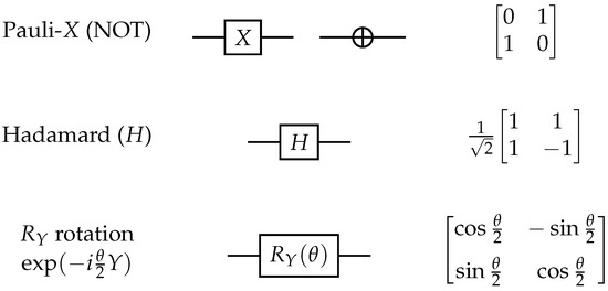
Figure 1. Single-qubit gates used in this paper and their corresponding matrices, which operate on the superposition state $\alpha |0⟩+\beta |1⟩$ written as the column vector ${\left[\begin{array}{cc}\alpha & \beta \end{array}\right]}^T$.

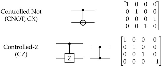
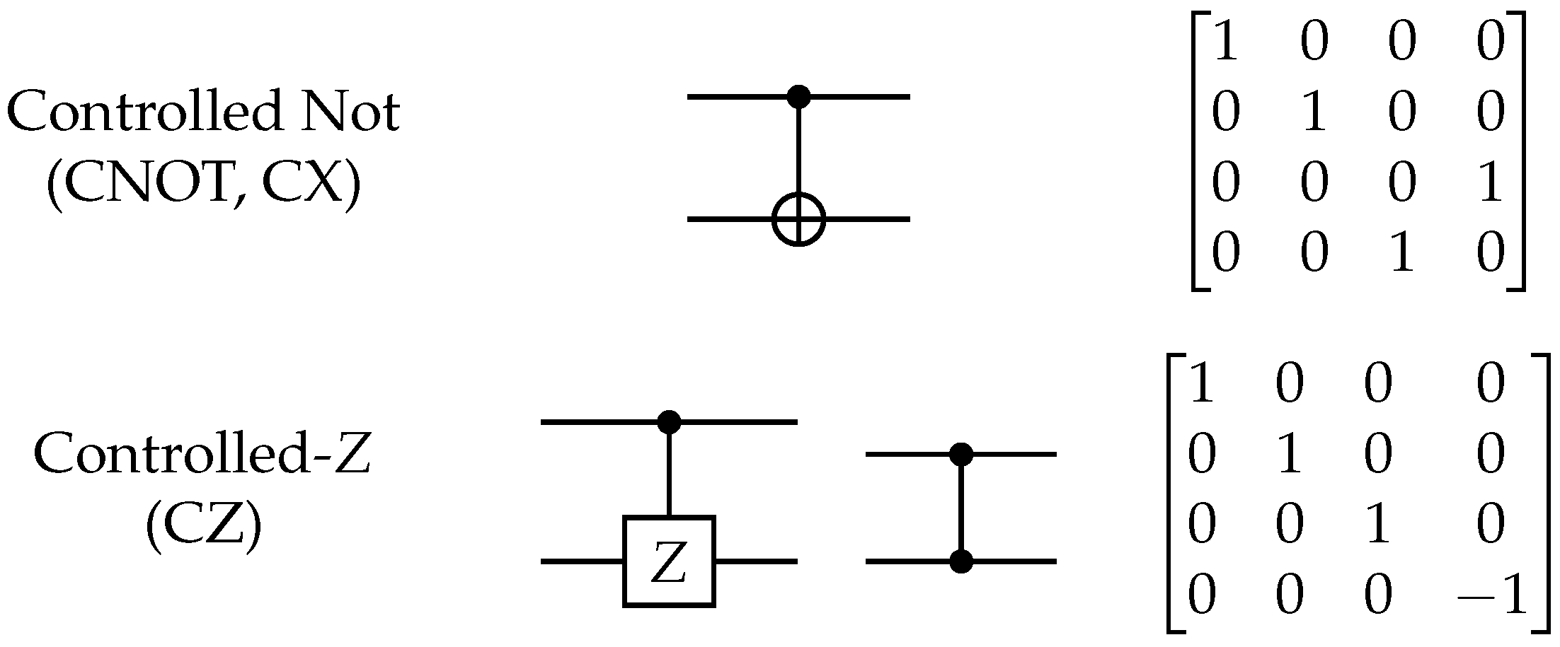
Figure 2. Two-qubit CNOT (controlled-X) and controlled-Z gates.

The Pauli-X gate is commonly used to flip a qubit between the $|0⟩$ and $|1⟩$ gates, which is why it is also sometimes called the quantum NOT gate. X-gates directed at different qubits can be used to prepare an input state representing a binary-valued vector: the state $|010\dots 001⟩$ is prepared by applying an X-gate to each of the qubits to be switched to the $|1⟩$ state.

The Hadamard (H) gate is commonly used to put a qubit into a superposition state; for example, it maps a qubit prepared in the state $|0⟩$ to the superposition $\frac{1}{\sqrt{2}}(|0⟩+|1⟩)$. Applying an H-gate to each qubit in an array is used to initialize a binary vector all of whose coordinates have a 50:50 chance of being observed in the $|0⟩$ or $|1⟩$ state.

The CNOT gate is a 2-qubit entangling gate, which acts upon the state $\alpha |00⟩+\beta |01⟩+\gamma |10⟩+\delta |11⟩$. In the standard basis, its behavior can be described as “performing a NOT operation on the target qubit if the control qubit is in state $|1⟩$”.

The Pauli-X, Hadamard, CNOT, and CX gates are self-inverse: performing these operations twice gives the identity map. These periodic properties are crucial for performing the binary arithmetic operations in the matrix–vector product of Section 3.

The $R_Y\left(\theta \right)$ rotates a single qubit through an angle $\theta$ around the Y-axis on the Bloch sphere (Nielsen and Chuang [6], Chapter 1). The angle $\theta$ can be varied, and optimizing these angles for many gates is the task of the variational algorithm in Section 4. The controlled-Z gate is similar to the CNOT gate and entangles two qubits; in the standard basis, its action is symmetric (in the sense that it does not matter which qubit is considered to be the control and which the target qubit).

3. Implementing the Matrix–Vector Product as a Quantum Circuit

This section introduces a quantum circuit that implements the binary-valued matrix–vector product $Ax$, where A is a matrix and x is a vector, and both have values in ${\mathbb{F}}_2$ as defined above.

The trick is to notice that binary arithmetic may be implemented with controlled-NOT operations. The NOT gate switches the state of an individual qubit between $|0⟩$ and $|1⟩$, and the $\mathrm{CNOT}$ gate performs such an operation only if the so-called control qubit is in state $|1⟩$. In particular, the $\mathrm{CNOT}$ gate acts on the two-qubit state $|y,z⟩$ as

$$\mathrm{CNOT}|y,z⟩=|y,y\oplus z⟩.$$

(1)

Now let $|x⟩=|x_1,x_2,\dots ,x_n⟩$ denote the n-qubit quantum state corresponding to x and notice that

$$Ax\equiv \left[\begin{array}{c}{a}_{11}{x}_1\oplus \dots \oplus a_{1n}{x}_n\\ ⋮\\ a_{m1}{x}_1\oplus \dots \oplus a_{mn}{x}_n\end{array}\right]mod2.$$

Thus the m-qubit state $|Ax⟩$ can be prepared by applying the quantum circuit

$$\mathcal{A}=\prod _{j=1}^n{\mathcal{A}}_j,\mathrm{with}{\mathcal{A}}_j=\prod _{i=1}^m\mathrm{CNOT}{(j,n+i)}^{a_{ij}}$$

(2)

to the tensor product $|x⟩|0⟩$. Here, $\mathrm{CNOT}(k,\mathsf{\ell })$ denotes a $\mathrm{CNOT}$ gate controlled by the $k^{\mathrm{th}}$ qubit and targeting the ${\mathsf{\ell }}^{\mathrm{th}}$ one. The product operator $\Pi$ in these definitions denotes composition, so it is implemented by applying the gates in sequence. Both products in Relation (2) may be taken in any order. We note that $\mathcal{A}$ requires $m+n$ qubits and N quantum gates, with N denoting the number of non-zero entries in A.

In particular, we obtain the following theorem.

Theorem 1.

Using$\mathcal{A}$as in Relation (2), with $|0⟩$ denoting the m-qubit all-zero state, and with $|x⟩|0⟩$ denoting the concatenation/tensor product of $|x⟩$ and $|0⟩$, we have

$$\mathcal{A}\left(|x⟩|0⟩\right)=|x⟩|Ax⟩.$$

Proof. 

The proof follows from an easy argument by induction on n that is left to the reader: the base case $n=1$ can be easily established for all m by verifying that the ith qubit in the output register is zero precisely when $a_{ij}=0$, and the inductive step follows from a quick calculation considering the inductive hypothesis and the action of the $\mathrm{CNOT}$ gate, as in Relation (1). □

Example 1.

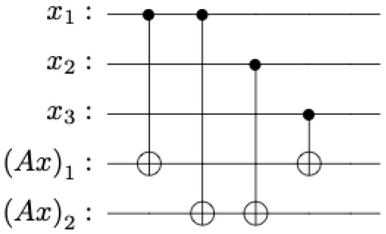
The following example elucidates Theorem 1. For concreteness, consider the $2\times 3$ matrix

$$A=\left[\begin{array}{ccc}1& 0& 1\\ 1& 1& 0\end{array}\right]sothatAx\equiv \left[\begin{array}{c}{x}_1\oplus x_3\\ x_1\oplus x_2\end{array}\right]mod2.$$

Then

$$\begin{array}{c}\hfill {\mathcal{A}}_1=\mathrm{CNOT}(1,4)\mathrm{CNOT}(1,5),{\mathcal{A}}_2=\mathrm{CNOT}(2,5),and{\mathcal{A}}_3=\mathrm{CNOT}(3,4),\end{array}$$

and therefore

$$\begin{array}{c}\hfill \mathcal{A}|x⟩|0,0⟩={\mathcal{A}}_3{\mathcal{A}}_2|x⟩|x_1,x_1⟩={\mathcal{A}}_3|x⟩|x_1,x_1\oplus x_2⟩=|x⟩|x_1\oplus x_3,x_1\oplus x_2⟩=|x,Ax⟩.\end{array}$$

The diagram in Figure 3 shows how the operator$\mathcal{A}$is implemented explicitly as a quantum circuit.

Figure 3. Quantum circuit implementing the operator $\mathcal{A}$ from Example 1.

These circuits work because the self-inverse behavior of the X and CNOT gates is ideal for binary arithmetic over ${\mathbb{F}}_2$. It is possible that the periodic nature of other gates could be used similarly to perform arithmetic operations over other finite fields, but such an adaptation is not straightforward unless we consider qudits instead of qubits, because the way several CNOT gates combine angles into a single target qubit does not perform like group addition for fields other than ${\mathbb{F}}_2$. More precisely, the X and $\mathrm{CNOT}$ gates rotate their target qubits through angles 0 and $\pi$, which is all we need for the 0 and 1 elements of ${\mathbb{F}}_2$, but if this is extended to a larger set of angles $2\pi /p$ for $p\ne 2$, the use of CNOT gates to combine different contributions into a single target qubit as in Figure 4 is nonlinear [7]. It follows that the coordinates of the output vector b are not the same as the sums of the various inputs ${\left(Ax\right)}_j$, except for the two-element field ${\mathbb{F}}_2$.

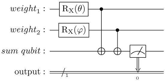
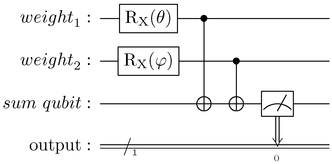
Figure 4. An “adder circuit” that combines the values of $\theta$ and $\varphi$ into the target qubit, whose probability of measuring a $|1⟩$ is ${sin}^2\left(\theta \right){cos}^2\left(\phi \right)+{cos}^2\left(\theta \right){sin}^2\left(\phi \right)$, as demonstrated in [8]. Note the structural similarity with the inputs to ${\left(Ax\right)}_0$ in Figure 3.

4. Solving the Linear System Using a Variational Quantum Algorithm

Now we propose a Variational Quantum Algorithm (VQA) designed to solve the linear system $Ax\equiv bmod2$. As with any VQA, there are two main ingredients: a variational ansatz and a cost function that serves as the optimization objective. The ansatz gives a circuit pattern or template with gate parameters (typically angles) that can be varied and optimized. In this report we consider one objective function and compare two different ansatze: a rotations ansatz specially designed for the task, and a more generic brickwork ansatz.

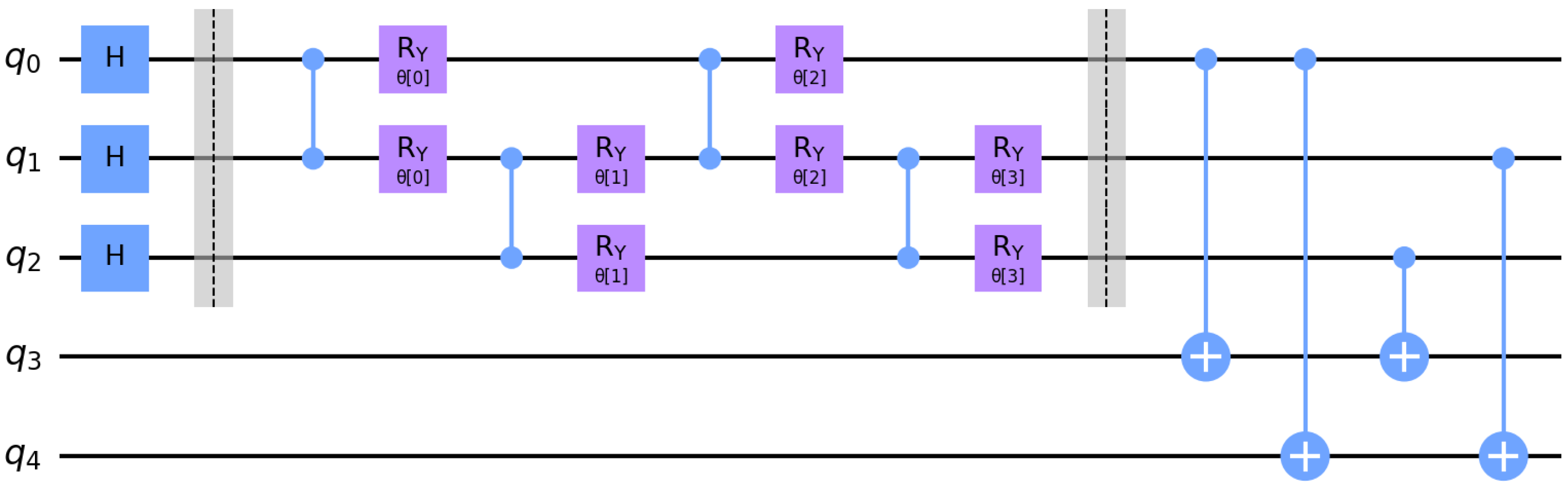
The system as a whole is called $\mathrm{Mod}2\mathrm{VQLS}$, which stands for Modulo 2 Variational Quantum Linear Solver. Figure 5 illustrates the full variational circuit evaluated by $\mathrm{Mod}2\mathrm{VQLS}$ when solving the linear system described in Example 1. In this case, the brickwork layout variational ansatz described in Section 4.2 is used, with 4 layers.

Figure 5. Variational circuit for solving $Ax=b$ as in Example 1 using a brickwork layout ansatz with 2 layers. The gray bars serve as visual aids helping th reader distinguish the different parts of the circuit: initial state creation, variational component, and matrix-vector product.

Our cost function here measures the overlap between the projector $|\psi \left(\theta \right)⟩⟨\psi \left(\theta \right)|$ and the subspace orthogonal to $|b⟩$, which is given by

$$\widehat{C}=\mathrm{tr}\left(|\psi \left(\theta \right)⟩⟨\psi \left(\theta \right)|(\mathrm{id}-|b⟩⟨b|)\right).$$

We note that this cost function has appeared before in [9] as Equation (3) in the setting of solving square linear systems with real entries.

Some algebra shows that $\widehat{C}$ can be evaluated by computing the expected energy of an Ising Hamiltonian:

$$\begin{array}{cc}\hfill \widehat{C}& =\mathrm{tr}\left(|\psi ⟩⟨\psi |(\mathrm{id}-|b⟩⟨b|)\right)=⟨\psi |(\mathrm{id}-|b⟩⟨b|)|\psi ⟩=1-{\left|⟨b|\psi ⟩\right|}^2,\hfill \end{array}$$

(3)

where we have omitted the dependence on $\theta$ for simplicity of notation. Notice that the second term is the expected value of the rank-1 Ising Hamiltonian $|b⟩⟨b|$ with eigenvalue 1 corresponding to the eigenstate $|b⟩$, computed with respect to the variational state $|\psi ⟩$. Although it may be difficult to express this Hamiltonian as a linear combination of tensor products of Pauli matrices, we do not need to construct or even to know it explicitly; all we need is an oracle that can lazily evaluate the Hamiltonian’s eigenvalues.

4.1. Rotations Ansatz

Now we turn to our variational ansatze. The first is a simple rotations pattern that is particularly well-suited for the Mod2VQLS cost function $\widehat{C}$. This ansatz is just a product of single-qubit rotations about the Y-axis; in particular, we take

$$V\left(\theta \right)=\prod _{j=1}^n{R}_Y^j\left({\theta }_j\right),$$

(4)

with $R_Y^j$ denoting an $R_Y$ rotation applied on the $j^{\mathrm{t}\mathrm{h}}$r qubit and each parameter $\theta \in {[-2\pi ,2\pi ]}^n$. This circuit is interesting because it does not add to the overall computational cost of each iteration, and it is amenable to direct mathematical analysis.

In particular, we can derive an explicit formula for the variational cost as a function of the circuit parameters.

Theorem 2.

For each $x\in {\mathbb{F}}_2^n$, define ${\alpha }_x\left(\theta \right)={\prod }_{j=1}^{n}cos{({\theta }_j/2)}^{(1-x_j)}sin{({\theta }_j/2)}^{x_j}$. In addition, let $A^{-1}\left(b\right)=\{x\in {\mathbb{F}}_2^n\mid Ax\equiv bmod2\}$ denote the inverse image of b under A. Then,

$$\widehat{C}\left(\theta \right)=1-\sum _{x\in A^{-1}\left(b\right)}{\alpha }_x{\left(\theta \right)}^2$$

with $|\psi \left(\theta \right)⟩=\mathcal{A}V\left(\theta \right)|0⟩$ and $V\left(\theta \right)$ denoting the ansatz defined by Relation (4).

Proof. 

The theorem follows from direct calculation. First, note that

$$R_Y\left({\theta }_j\right)|0⟩=cos({\theta }_j/2)|0⟩+sin({\theta }_j/2)|1⟩.$$

So, a quick induction, left to the reader as an exercise, shows that

$$V\left(\theta \right){|0⟩}^{\otimes n}=\underset{j=1}{\overset{n}{⨂}}\left(R_Y^j\left({\theta }_j\right)|0⟩\right)=\underset{j=1}{\overset{n}{⨂}}\left(cos({\theta }_j/2)|0⟩+sin({\theta }_j/2)|1⟩\right)=\sum _{x\in {\mathbb{F}}_2^n}{\alpha }_x\left(\theta \right)|x⟩.$$

Combined with Theorem 1, the last equation yields an expression for our variational quantum state:

$$|\psi \left(\theta \right)⟩=\mathcal{A}V\left(\theta \right){|0⟩}^{\otimes n}=\sum _{x\in {\mathbb{F}}_2^n}{\alpha }_x\left(\theta \right)|x⟩|Ax⟩.$$

(5)

We use this expression to compute the variational cost with respect to $|\psi \left(\theta \right)⟩$. In particular, let

$$\mathcal{H}=I\otimes |b⟩⟨b|=\sum _{y\in {\mathbb{F}}_2^n}|y⟩⟨y|\otimes |b⟩⟨b|$$

and use Relation (3) to write

$$1-\widehat{C}\left(\theta \right)={\left|⟨b|\psi \left(\theta \right)⟩\right|}^2=⟨\psi \left(\theta \right)|\mathcal{H}|\psi \left(\theta \right)⟩.$$

Now, since ${\alpha }_x\left(\theta \right)$ is real, we see that

$$\begin{array}{cc}\hfill ⟨\psi \left(\theta \right)|\mathcal{H}|\psi \left(\theta \right)⟩& =\sum _{x,y}{\alpha }_x\left(\theta \right){\alpha }_y\left(\theta \right)⟨x|y⟩⟨Ax|b⟩⟨b|Ay⟩\hfill \\ \hfill & =\sum _{x\in {\mathbb{F}}_2^n}{\alpha }_x{\left(\theta \right)}^2{\left|⟨Ax|b⟩\right|}^2\hfill \\ \hfill & =\sum _{x\in A^{-1}\left(b\right)}{\alpha }_x{\left(\theta \right)}^2,\hfill \end{array}$$

so $\widehat{C}\left(\theta \right)=1-{\sum }_{x\in A^{-1}\left(b\right)}{\alpha }_x{\left(\theta \right)}^2$ as desired. □

Moreover, we can obtain a similar formula for the gradient of the cost function with respect to the circuit parameters.

Theorem 3.

For each $j=1,\dots ,n$, the cost function $\widehat{C}\left(\theta \right)$ varies like

$$\frac{\partial }{\partial {\theta }_j}\widehat{C}\left(\theta \right)=\sum _{x\in A^{-1}\left(b\right)}{(-1)}^{1-x_j}{\alpha }_x\left(\theta \right){\alpha }_{x\oplus e_j}\left(\theta \right)$$

with respect to ${\theta }_j$. Here, ⊕ denotes binary addition over ${\mathbb{F}}_2^n$ and $e_j$ denotes the jth standard basis vector in ${\mathbb{F}}_2^n$.

Proof. 

The theorem follows from a direct computation using the chain rule. The key is to notice that differentiating ${\alpha }_x$ swaps a sine for a cosine and vice versa; for instance, if $x_j=0$, and we fix $c_k=cos\left(\frac{{\theta }_k}{2}\right)$ and $s_k=sin\left(\frac{{\theta }_k}{2}\right)$ for simplicity of notation, we see that

$$\frac{\partial }{\partial {\theta }_j}{\alpha }_x\left(\theta \right)=\frac{\partial }{\partial {\theta }_j}\left[\prod _{k=1}^n{c}_k^{1-x_k}{s}_k^{x_k}\right]=\frac{-s_j}{2}\left[\prod _{k\ne j}{c}_k^{1-x_k}{s}_k^{x_k}\right]=-\frac{1}{2}{\alpha }_{x\oplus e_j}\left(\theta \right).\square$$

Theorem 3 helps us understand the critical points on the variational cost landscape. In particular, it shows that the gradient $\nabla \widehat{C}\left(\theta \right)$ is smooth, and moreover, each of its entries is a trigonometric polynomial on the $2n$ variables $c_j=cos\left(\frac{{\theta }_j}{2}\right)$ and $s_j=sin\left(\frac{{\theta }_j}{2}\right)$, for $j=1,\dots ,n$. Thus, every critical point of the cost surface satisfies $\nabla \widehat{C}=0$. When combined with the Pythagorean identities $c_j^2+s_j^2=1$, the equation $\nabla \widehat{C}=0$ characterizes an algebraic variety defined by $2n$ polynomials in $2n$ variables. Hence Bezout’s Theorem [10], Chapter 2 implies that $\widehat{C}$ has at most ${\left(2n\right)}^n·2^n={\left(4n\right)}^n$ real extrema.

It is interesting to note that when $(c_j,s_j)$ is an $8n$-th root of unity, our variational cost can be written in terms of quantum integers or q-integers, which are ubiquitous in q-calculus, the representation theory of quantized enveloping algebras and quantum groups, and in the theory of crystal bases, amongst others [11,12,13,14,15]. We conjecture that these points characterize the extrema of our cost function. The conjecture is motivated by the size of the variety characterized by $\nabla \widehat{C}=0$ together with the Pythagorean identities as computed by Bezout’s Theorem and by the explicit computations summarized by Theorem 5.

Definition 1.

For any complex $q\ne 1$ and any integer n, the quantum integer or q-integer ${\left[n\right]}_q$ is defined by

$${\left[n\right]}_q=\frac{q^n-q^{-n}}{q-q^{-1}}=q^{n-1}+q^{n-3}+\dots +q^{3-n}+q^{1-n}.$$

In this setting, quantum integers appear in the coefficients ${\alpha }_x\left(\theta \right)$. In particular, let ${\theta }_j=\frac{\pi }{2n}{p}_j$ for any $p_j\in \{0,1,\dots ,4n-1\}$, let $\xi =e^{\frac{i\pi }{4n}}$ denote a primitive $8n$-th root of unity, and notice

$$cos{({\theta }_j/2)}^{1-x_j}sin{({\theta }_j/2)}^{x_j}=\frac{\left(i^{1-x_j}{e}^{\frac{i\pi p_j}{2}}\right)-{\left(i^{1-x_j}{e}^{\frac{i\pi p_j}{2}}\right)}^{-1}}{2i}=\frac{{[2n(1-x_j)+p_j]}_{\xi }}{{\left[2n\right]}_{\xi }}.$$

We use the last identity to prove the existence of globally optimal parameters for our variational circuit. It is important to observe these guarantees are not typically offered by VQAs; for instance, QAOA can only guarantee such parameters in the limit of infinite circuit depth.

We will need the following identities.

Lemma 4.

If $\xi =e^{\frac{i\pi }{4n}}$ denotes a primitive $8n$-th root of unity, then the following identities relating ξ-integers hold:

$${\left[3n\right]}_{\xi }={\left[n\right]}_{\xi }=\frac{{\left[2n\right]}_{\xi }}{\sqrt{2}},and{\left[4kn\right]}_{\xi }=0foranyk\in \mathbb{Z}.$$

Proof. 

The lemma follows from direct calculation. For example,

$${\left[3n\right]}_{\xi }=\frac{{\xi }^{3n}-{\xi }^{-3n}}{\xi -{\xi }^{-1}}=\frac{2i}{\xi -{\xi }^{-1}}·sin\left(3n·\frac{\pi }{4n}\right)=\frac{2i}{\xi -{\xi }^{-1}}·sin\left(n·\frac{\pi }{4n}\right)={\left[n\right]}_{\xi }.$$

The second equality follows because $sin\left(n·\frac{\pi }{4n}\right)=1/\sqrt{2}$ and ${\xi }^{2n}=i$, so that ${\xi }^{2n}-{\xi }^{-2n}=2i$. The last equality holds because $\xi$ is an $8n$-th root of unity; in particular, ${\xi }^{4kn}={\xi }^{-4kn}$. □

Theorem 5.

Let $\theta =\frac{\pi }{2n}p$ for some $p\in {\mathbb{Z}}^n$. First, suppose $p=2n{x}^{\prime }$ for some $x^{\prime }\in {\{0,1\}}^n$. Then, $\widehat{C}\left(\theta \right)=0$ is a global minimum of $\widehat{C}:{\mathbb{R}}^n\to \mathbb{R}$ if $x^{\prime }$ satisfies $A{x}^{\prime }=b$; otherwise, $\widehat{C}\left(\theta \right)=1$ is a global maximum of the cost function.

Now assume $p_1=\dots =p_n=kn$ for some odd integer k and let $\mathrm{rk}\left(A\right)$ denote the rank of A over ${\mathbb{F}}_2$. In this case, $\widehat{C}\left(\theta \right)=1-2^{-\mathrm{rk}\left(A\right)}$.

Proof. 

First, notice our cost function is non-negative; for any $\theta \in {\mathbb{R}}^n$, we have

$$\widehat{C}\left(\theta \right)=1-\sum _{x\in A^{-1}\left(b\right)}{\alpha }_x{\left(\theta \right)}^2\ge 1-\sum _{x\in {\mathbb{F}}_2^n}{\alpha }_x{\left(\theta \right)}^2=1-⟨\psi \left(\theta \right)|\psi \left(\theta \right)⟩=0.$$

This follows from Relation (5), which writes $|\psi \left(\theta \right)⟩$ as a superposition over a tensor product of computational basis states with amplitudes given by ${\alpha }_x\left(\theta \right)$. In addition, $\widehat{C}$ is bounded above by 1 because each ${\alpha }_x{\left(\theta \right)}^2$ is non-negative. This means $0\le \widehat{C}\left(\theta \right)\le 1$ for every $\theta \in {\mathbb{R}}^n$.

Thus, to prove the first claim, it remains to be shown that when $p=2n{x}^{\prime }$, the cost function vanishes if $x^{\prime }$ belongs to the inverse image $A^{-1}\left(b\right)$ and it is unity otherwise. This follows from direct calculation:

$$\begin{array}{cc}\hfill 1-\widehat{C}\left(\theta \right)& =\sum _{x\in A^{-1}\left(b\right)}{\alpha }_x{\left(\theta \right)}^2=\frac{1}{{\left[2n\right]}_{\xi }^{2n}}\sum _{x\in A^{-1}\left(b\right)}\prod _{j=1}^n{\left[2n(1-x_j+x_j^{*})\right]}_{\xi }^2\hfill \\ \hfill & =\frac{1}{{\left[2n\right]}_{\xi }^{2n}}\sum _{x\in A^{-1}\left(b\right)}{\delta }_{x,x^{\prime }}{\left[2n\right]}_{\xi }^{2n}\hfill \\ \hfill & =\sum _{x\in A^{-1}\left(b\right)}{\delta }_{x,x^{\prime }}.\hfill \end{array}$$

Note that the product in the second equality vanishes whenever $x\ne x^{\prime }$ because ${\left[4n\right]}_{\xi }=0$.

For the second claim, write $k=4m+r$ for some integer m and with $r=1,3$. Now recall the well-known ‘summation rule’ ${[s+t]}_q=q^s\left[t\right]+q^{-t}{\left[s\right]}_q$ for quantum integers ([12], Relation V1.1.2). When combined with Lemma 4, the summation rule implies

$${\left[kn\right]}_{\xi }={\xi }^{rn}{\left[4mn\right]}_{\xi }+{\xi }^{-4mn}{\left[rn\right]}_{\xi }={(-1)}^m{\left[rn\right]}_{\xi }.$$

(6)

In addition, note that if $r=3$, Relation (6) implies ${\left[(r+2)n\right]}_{\xi }={\left[5n\right]}_{\xi }=-{\left[rn\right]}_{\xi }$. Thus, if ${\mathbf{1}}^{T}x\in \mathbb{Z}$ denotes the (integer) sum of the elements of x, we see that

$$\begin{array}{cc}\hfill 1-\widehat{C}\left(\theta \right)& =\sum _{x\in A^{-1}\left(b\right)}{\alpha }_x{\left(\theta \right)}^2=\frac{1}{{\left[2n\right]}_{\xi }^{2n}}\sum _{x\in A^{-1}\left(b\right)}\prod _{j=1}^n{[2n(1-x_j)+kn]}_{\xi }^2\hfill \\ \hfill & =\frac{1}{{\left[2n\right]}_{\xi }^{2n}}\sum _{x\in A^{-1}\left(b\right)}{\left({\left[(k+2)n\right]}_{\xi }^{n-{\mathbf{1}}^{T}x}{\left[kn\right]}_{\xi }^{{\mathbf{1}}^{T}x}\right)}^2\hfill \\ \hfill & =\frac{1}{{\left[2n\right]}_{\xi }^{2n}}\sum _{x\in A^{-1}\left(b\right)}{\left({\left[(r+2)n\right]}_{\xi }^{n-{\mathbf{1}}^{T}x}{\left[rn\right]}_{\xi }^{{\mathbf{1}}^{T}x}\right)}^2\hfill \\ \hfill & =\frac{1}{{\left[2n\right]}_{\xi }^{2n}}\sum _{x\in A^{-1}\left(b\right)}{\left[n\right]}_{\xi }^{2n}\hfill \\ \hfill & =\frac{|A^{-1}\left(b\right)|}{{\sqrt{2}}^{2n}}.\hfill \end{array}$$

In the fourth equality we used Lemma 4 to simplify ${\left[(r+2)\right]}_{\xi }^2={\left[rn\right]}_{\xi }^2={\left[n\right]}_{\xi }^2$. In the fifth equality we applied Lemma 4 again, this time substituting ${\left[n\right]}_{\xi }={\left[2n\right]}_{\xi }/\sqrt{2}$.

To conclude, we recall the solution set $A^{-1}\left(b\right)$ is an affine space in ${\mathbb{F}}_2^n$ with one point for each element of the kernel of A. Hence, if we let $\mathrm{null}\left(A\right)$ denote the dimension of $kerA$ over ${\mathbb{F}}_2$ and we recall the Rank–Nullity Theorem we obtain the desired result:

$$\widehat{C}\left(\theta \right)=1-\frac{|A^{-1}\left(b\right)|}{{\sqrt{2}}^{2n}}=1-\frac{2^{\mathrm{null}\left(A\right)}}{2^n}=1-2^{-\mathrm{rk}\left(A\right)}.\square$$

4.2. Brickwork Ansatz

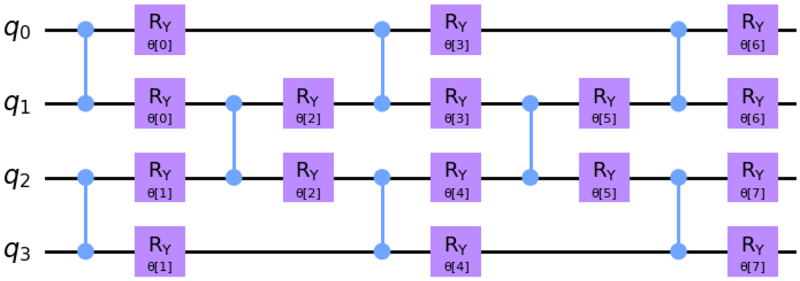
The other variational ansatz we consider comprises a brickwork layout of parametrized two-qubit gates. For instance, Figure 6 illustrates a brickwork layout ansatz with a depth of 5 layers on 4 qubits. The two-qubit ‘brick’ design was used by authors including [9] for general linear solving and [16] for electron simulation. Various other general-purpose ansatz designs could be tried.

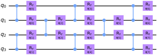
Figure 6. A brickwork layout ansatz on 4 qubits with a depth of 5 layers.

With enough layers, it should be possible for the brickwork ansatz to provide solutions to the equation $Ax=b$, and intuitively, we expected that convergence would be slower but that the method might find more solutions overall. In practice, the convergence was considerably slower, and in most cases, the number of extra solutions found was modest.

4.3. Variational Parameter Optimization

Along with the quantum circuits, hybrid systems like Mod2VQLS rely on classical algorithms to optimize the variational parameters (for example, the $\theta$ parameters in the examples so far). Parameter optimization in variational quantum circuits has become an important topic in quantum machine learning, partly because it is a signification barrier to overcome if variational quantum circuits are to deliver valuable applications on NISQ hardware.

A considerable challenge here is that automatic differentiation (“autodiff”) is not straightforward on quantum computers: finite-difference methods require too many nearby calculations, and even when an analytic expression for gradients is available using a ‘parameter shift rule’, these expressions have to be evaluated separately for each parameter ([3], §5.3). As fresh problems are encountered, it is possible that quantum computers are not well-suited to computing gradients, and that there is no quantum approach to training variational networks that is as generally effective as classical backpropagation [17].

Simplex-based methods are a well-established alternative to gradient-based methods. In the simple one-dimensional case, binary search is an elementary example. In more dimensions, an n-dimensional simplex is the convex hull of n linearly independent vertices, and the search algorithm converges by iteratively partitioning the simplex and reducing to a smaller simplex that contains the desired solution. (For example, a triangle subdivided by a suitable line, or a tetrahedron subdivided by a suitable plane.) This is the backbone of many procedures, including the famous 1965 simplex algorithm of Nelder and Mead [18]. Nelder–Mead can sometimes be improved using interpolation based on the values of the objective function at the vertices, leading to the COBYLA algorithm published in 1994 [19]. SciPy’s COBYLA implementation was used in the Mod2VQLS experiments presented below.

4.4. Alternatives

There are several alternatives and ways this design could be varied. With the quantum parts of the system, one could use a different two-qubit block in the brickwork layout ansatz. More generally, we could use a different ansatz altogether. In particular, it might be beneficial to incorporate linear-algebraic information into the ansatz, such as something that encourages the superposition to be orthogonal to the range of A, in case $b=0$. Also, a swap test could be used for computing $\widehat{C}$ as part of the quantum circuit itself [20]. This may serve as a way to mitigate the measurement error, at the cost of requiring additional qubits.

For the classical parts of the system, we have discussed the reason for choosing a simplex-based rather than a gradient-based optimizer. This broad-strokes distinction leaves many opportunities for more specific combinations to be evaluated. Other optimization algorithms including SPSA (gradient-free) and AMSGrad (gradient-based) have also been evaluated by Pellow-Jarman et al. [21]. Finding ideal combinations of classical optimizers and quantum circuit ansatze is likely to remain an important research topic.

5. Experimental Results

This section describes the results of experiments evaluating the performance of Mod2VQLS solvers using both the rotation and brickwork ansatze.

In each dimension from 1 to 9, we generated ten consistent binary linear systems by constructing $n\times n$ matrices A and n-vectors x with independent and uniformly selected entries in $\{0,1\}$ and then computing $Ax=b$. Then, we solved the systems using Mod2VQLS, using both the brickwork and rotation ansatze. Solving a linear system entails optimizing the model’s variational parameters and then measuring the optimized state $|\psi \left({\theta }^{*}\right)⟩$. We tested all the computational states observed in the optimized superposition in order to determine whether they were valid solutions to the linear system in question. We counted the number of distinct valid and invalid solutions proposed, as well as the average number of iterations required for convergence of the variational method. We used SciPy 1.11’s COBYLA implemetation to update the variational parameters in our circuits; we note this optimization routine only requires a single quantum circuit execution per iteration. Circuits were coded and simulated using the Qiskit Python package [22].

In the brickwork case, the number of layers in the variational ansatz is an extra configuration parameter. From experimenting, we found that at least two layers were needed and that matching the number of layers/parameters to the number of dimensions produced a reasonable tradeoff between solution iterations and correctness.

Our results are presented in Table 1. The rotations ansatz performed quite simply and effectively, always finding a correct solution, and occasionally finding more than one, with a reasonably small number of iterations. The rotations ansatz proposed no invalid solutions. The brickwork ansatz was more costly and error-prone, using more iterations and producing some invalid solutions. The brickwork ansatz was also able to find a greater variety of valid solutions, though not dramatically so.

Table 1. Experimental results using brickwork and rotation ansatze in various dimensions, using 10 randomly generated matrices in each dimension, showing how many valid and invalid solutions were proposed, and how many iterations were used, by each method.

	Brickwork Ansatz				Rotation Ansatz
Dim	Solved	Valid	Invalid	Average	Solved	Valid	Invalid	Average
		Solns	Solns	Iterations		Solns	Solns	Iterations
1	8	8	2	1	10	10	0	2
2	10	16	4	1.7	10	14	0	3.7
3	10	14	5	1	10	11	0	9.2
4	9	9	1	38.8	10	11	0	16.3
5	10	19	0	93.2	10	11	0	17.3
6	10	15	0	177.4	10	11	0	18.9
7	10	11	1	86.2	10	10	0	24.6
8	10	11	0	120.2	10	10	0	29.4
9	10	10	0	122.4	10	10	0	33.5

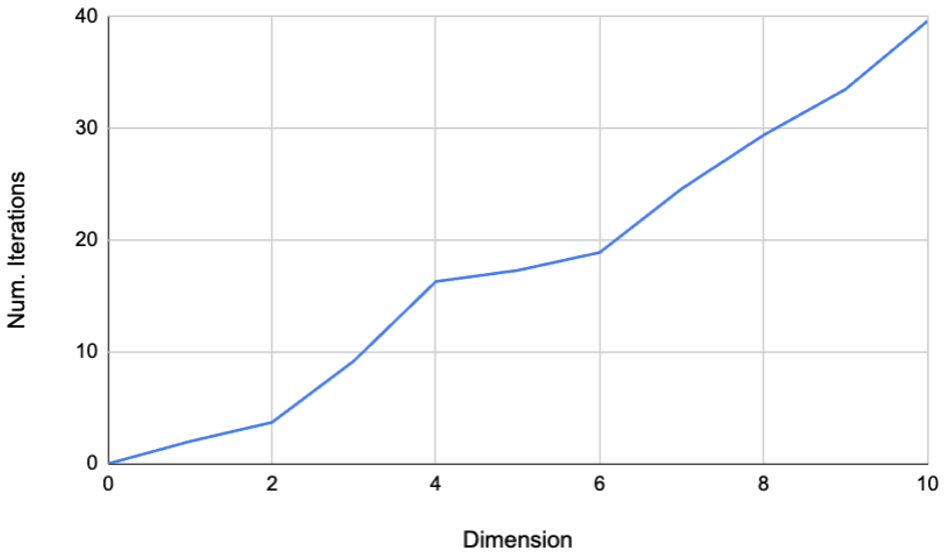
Figure 7 shows the growth in the number of iterations used by Mod2VQLS with the rotations ansatz. The growth is roughly linear in small dimensions, with a slope of (just under) 4. This allows for comparison with block Wiedemann, as explained in Section 6 below.

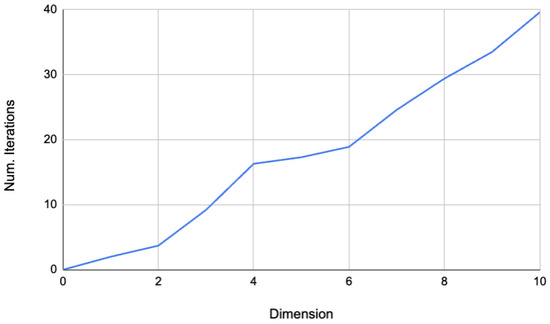
Figure 7. Average number of iterations needed to find a solution for each dimension using the rotations ansatz. The number of iterations grows approximately linearly, with a slope just under 4.

These experiments demonstrate proof-of-concept, in that the Mod2VQLS system does find correct solutions. They also demonstrate that there are performance tradeoffs, and that different choices of ansatz may be appropriate, depending on whether the task requires searching for any solution, or a more exhaustive search for all solutions.

These results are preliminary. The Mod2VQLS algorithm should be tested on larger systems of linear equations and compared with the results of classical solvers. The robustness of the circuits at larger scales with different kinds of noise has not yet been analyzed.

6. Related Classical and Quantum Methods for Solving Linear Systems

This section compares Mod2VQLS with quantum alternatives for solving systems of linear equations and classical alternatives for solving systems of binary linear equations.

6.1. Quantum Linear Solvers

Important families of quantum linear solvers are based on the renowned HHL algorithm of Harrow, Hasidim, and Lloyd [23], and the VQLS (Variational Quantum Linear Solver) algorithm of [9]. The HHL algorithm is an exact method for solving linear equations, with several papers proposing applications and improvements including [24], though also with significant caveats [25]. The VQLS approach is more recent, from the current era where variational methods are expected to perform well on real NISQ hardware, which has already encouraged subsequent research into VQLS, including the use of dynamic ansatze [26], comparing different optimizers [21], and applications to differential equations [27].

Mod2VQLS is different from these methods, particularly with its support for binary vectors, and non-square matrices. To date, works on matrix multiplication and solving linear equations using quantum computing have addressed the cases of real- and complex-valued matrices. (This is sometimes stated explicitly, and sometimes implied by the assumption that the vector coordinates are represented by complex amplitudes.) The recent work of [27] adapts the VQLS of [9] to finite-element methods for solving differential equations, but here the ‘elements’ are subdomains supporting a function, not elements of a finite field, and the functions in question are still continuous. As far as we know, our proposal here is the first attempt to address this problem with matrices over ${\mathbb{F}}_2$, or any finite field.

In addition, $\mathrm{Mod}2\mathrm{VQLS}$ can tackle matrices of any size and rank, whereas both HHL and VQLS are restricted to square matrices with full rank. This again is sometimes stated explicitly, and sometimes implied by the assumption that the matrix operator A is a quantum unitary operator. Indeed, the runtime of both HHL and VQLS depends on the condition number of the coefficient matrix, so effectively they assume the coefficient matrix is not only invertible, but robustly so (well-conditioned). When A is square, and moreover enjoys additional structural properties like invertibility, symmetry, or positive-definiteness, faster iterative methods including various Krylov subspace iterations and conjugate gradient are available [28].

The ability to work with matrices of different sizes and ranks is especially beneficial for solving problems where the matrix sizes are not fixed in advance. A case-in-point is the integer factoring problems investigated by [2], which motivated the development of $\mathrm{Mod}2\mathrm{VQLS}$. In this application, each equation (each row of the matrix A) is discovered independently in a massively parallel data collection phase. We are not looking for a unique solution to a fixed system of equations, but any solution to any subset of this system of equations. The $\mathrm{Mod}2\mathrm{VQLS}$ works especially well for this, because the optimized variational circuit produces a superposition over multiple solutions to $Ax=b$.

On the flip side, while HHL and VQLS promise an exponential speed-up over classical solvers, because they leverage a dense amplitude encoding that requires ${log}_{2}n$ qubits to represent the linear system $A^{\prime }{x}^{\prime }=b^{\prime }$ with an $n\times n$ coefficient matrix $A^{\prime }$, $\mathrm{Mod}2\mathrm{VQLS}$ can only promise a polynomial speed-up over the fastest-known classical solvers (which are already polynomial), because $\mathrm{Mod}2\mathrm{VQLS}$ requires circuits with $m+n$ qubits for solving the system $Ax=b$ with an $m\times n$ coefficient matrix A. Thus, it is important to note that Mod2VQLS promises at most a polynomial, not an exponential speed-up. Also, the ability to work with non-square matrices comes at a computational cost: as seen in Figure 3, we produce a mapping from ${\mathbb{F}}_2^n$ to ${\mathbb{F}}_2^m$ using $n+m$ qubits, but seen as a whole, the circuit is really a reversible unitary transformation on the space ${\mathbb{C}}^{2(n+m)}$. So, the ability to map between spaces of different dimensions in Mod2VQLS comes at the cost using disjoint sets of qubits for the input and output spaces.

6.1.1. Specific Differences from HHL

The $\mathrm{Mod}2\mathrm{VQLS}$ encoding furnishes several advantages that address the HHL caveats delineated by [25]. For starters, in HHL the load vector $b^{\prime }$ must be loaded onto the quantum processor and this task in itself may require an exponential number of steps (with respect to the number of qubits in the circuit) ([25], Caveat 1). By contrast, in our setting the load vector b is merely an m-bit string so it corresponds to an m-qubit computational basis state. As such, it can be efficiently loaded on the quantum computer using at most m NOT or Pauli-X gates, although it turns out it is not even necessary to load b onto the quantum processor in our current implementation.

Moreover, HHL assumes that the quantum computer can apply the unitary operator $e^{-i{A}^{\prime }t}$ efficiently for various values of t ([25], Caveat 2). In our setting, the closest analog is applying the matrix–vector product operator defined below, and doing so requires precisely N two-qubit gates, where N is the number of non-zero entries in A. The complexity here indicates that $\mathrm{Mod}2\mathrm{VQLS}$ directly benefits from the sparsity of A, which is useful in applied settings where one typically deals with large, (very) sparse matrices. For instance, the matrices encountered in recent large factoring calculations have millions of rows and columns, but only a few hundred non-zero entries per row.

Finally, extracting the solution vector $x^{\prime }$ upon executing the HHL algorithm requires an exponential number of circuit measurements ([25], Caveat 4). Again, the exponential here is with respect to the number of qubits in the HHL circuit. By contrast, in our modulo 2 setting the solution vector x is an n-bit string, which corresponds to an n-qubit computational basis state, so it can be read off from the optimized quantum ansatz using a fixed number of shots. An added benefit of our method is that the optimized quantum ansatz obtained upon running $\mathrm{Mod}2\mathrm{VQLS}$ is a superposition over computational basis states corresponding to every possible solution to $Ax=b$, so we can effectively sample the solution set by measuring the optimized quantum state. This is quite useful in the factoring application, where we typically need to find more than one element in the kernel of the coefficient matrix in order to build a factor.

6.1.2. Specific Differences from VQLS

There are a few additional differences that distinguish Mod2VQLS from the VQLS of Bravo-Prieto et al. [9] and subsequent developments. They use a dense encoding, which means that their cost function can be evaluated by executing quantum circuits with a logarithmic number of qubits. This is in contrast to our encoding, which requires a linear number of qubits. With the particular implementation details of the VQLS routine explained in [9] in mind, we see that our encoding has several benefits. For instance, in this context $\mathcal{A}$ is a unitary operation that can be performed using N gates, where N is the number of non-zero entries in the coefficient matrix. By contrast, the A operator in [9] is a linear combination of L unitaries, and L may be exponential in the number of qubits in their circuit. Moreover, the authors do not explain how to achieve such a decomposition in general; however, in Appendix A, they provide some hints for how to proceed when the coefficient matrix is sparse. In this section, they assume access to some oracle ${\mathcal{O}}_A$ that can effectively query the entries of A. Regardless, it is not clear how to implement this oracle and indeed the authors comment that, “The gate complexity of both of these strongly depends on the form and precision with which the matrix elements of A are specified” ([9], Appendix A).

Also in [9], the cost function ${\widehat{C}}_G$ vanishes when the norm of $|\psi ⟩$ vanishes, making it deficient in the sense that non-solutions to $Ax\equiv bmod2$ correspond to local extrema. By contrast, the variational state $|\psi \left(\theta \right)⟩$ used here is normalized because $\mathcal{A}V\left(\theta \right)$ is a unitary operation. Thus, there is no need to normalize the cost function, as in Equation (5) of [9] and consider the more complicated so-called local cost functions.

6.2. Classical Approach to Mod2 Linear Solving

Lacking prior literature on quantum binary linear solvers, we instead compare Mod2VQLS with the computational complexity of the block Wiedemann method, which is the fastest known classical algorithm for dealing with sparse unstructured systems over finite fields [29]. This method requires a linear number of matrix–vector multiplications plus a quadratic number of arithmetic operations in ${\mathbb{F}}_2$. In fact, large-scale implementations, like the one leveraged in the record-breaking RSA-240 calculation described in [5], have used $\ge 3n$ matrix–vector multiplications and it is not known if less than $2n$ can be used [30].

In our quantum setting, we consider the cost of executing our matrix–vector product circuit $\mathcal{A}$ from Section 3. The results from our numerical experiments using the rotations ansatz described in Section 4.1, as recorded in Table 1, indicate that the gate complexity of our simple quantum algorithm is on par with the state-of-the-art block Wiedemann approach: the number of matrix–vector multiplications needed to achieve a solution is linear in the system dimension and we do not require the additional quadratic number of field operations or linear storage. (However, our method requires at least one qubit per variable, so large-scale systems encountered in practice will require larger quantum computers).

7. Applications of Mod2VQLS and Related Techniques

Mod2VQLS was motivated by the use of modulo 2 linear algebra in integer factorization [2]. In this use-case, the goal is to find relations of the form $a^2\equiv b^{2}modn$, by multiplying various equations with known factors to obtain suitable $a^2$ and $b^2$. This requires that exponents of all the factors in the prime factorizations of both $a^2$ and $b^2$ are even; thus, assembling such a combination by multiplying several equations becomes translated into finding a suitable binary vector x so that $Ax\equiv 0\in {\mathbb{F}}_2^n$. The surprising importance of this ‘playing with numbers’ game is explained by Pomerance [1].

In the integer factorization application, the dimension n is determined by the number of (small) prime factors used in the ‘factor basis’ used to search for nearby composite numbers. The number of such relations determines the number of rows of A and the dimension m of the target space. This number is unknown at the beginning of the process; ideally, using the smallest number of relations possible reduces the burden on the ‘search phase’ of the algorithm, but this number is often large in practice. Hence it was a requirement for Mod2VQLS to work with a range of dimensions, and in particular, without the square matrix constraint that the number of equations must be equal to the number of unknowns.

The are other applications for binary linear solvers as well as integer factoring. The solution of some Boolean satisfiability problems can be optimized using Gaussian elimination with binary arithmetic, especially for cases with XOR constraints [31]. (Quantum approaches to more general Boolean satisfiability problems are surveyed by Alonso et al. [32].) Applications in cryptography and cryptanalysis, such as finding inverses of elements in the finite field $GF\left(2^m\right)$, have encouraged research on optimizing solutions of binary linear systems [33,34]. A component that solves linear systems modulo 2 is therefore required in various applications. Choosing an optimal approach typically depends on features including the dimension, number of equations, and sparsity; research on this problem is ongoing [35]. While it is unlikely that Mod2VQLS would have a significant enough advantage over block Wiedermann to motivate the expense of developing quantum computers for this purpose, it is much more likely that large-scale quantum computers will become commercially available for a range of applications, and that Mod2VQLS will have particular niches in this environment.

More generally, computations over the field ${\mathbb{F}}_2$ are fundamental in information and coding theory, and the data structures used sometimes overlap with work in quantum computing. For example, low-density parity-check (LDPC) codes work by comparing values between “value nodes” and “check nodes” in a bipartite graph [36,37]. Quantum graph learning is also a current field of research [38,39], and there are various proposed methods for developing quantum LDPC codes [40,41]. These methods involve various operations over ${\mathbb{F}}_2$, most of which do not involve solving complete sets of equations. An extra consideration is that some quantum processes can be parallelized in ways that enhance the security of distributed information [42], so there may be incentives for using quantum computers for specific system processes, beyond the traditional goals of reducing computational complexity and speeding-up classically intractable computations. As described in Section 3 above, the simple circuit design for computing the product of a matrix and a vector over ${\mathbb{F}}_2$ is the heart of the Mod2VQLS system, and components like this may end up being put to many different uses as the quantum computing ecosystem develops.

8. Conclusions

Variational quantum circuits provide design patterns that can be applied to a range of mathematical problems, especially ones that can be expressed as optimization problems with respect to some cost function. This paper demonstrated the Mod2VQLS system, which applies this design pattern to the problem of solving linear systems modulo 2. The key ingredients are a circuit for computing the matrix multiplication, a variational ansatz including parameters to optimize, and a classical optimization process. The rotation ansatz provided the most direct path to results, largely because its simple design made it amenable to analytical methods.

At the scales available to quantum computers today, the results here are potentially promising, but do not compete with classical solvers. The goal of this research is to investigate potential advantages at larger scale: we expect that medium-scale quantum computers will find their first regular commercial uses as part of larger hybrid pipelines. Understanding the quantum opportunities, and in particular, their scaling properties on real data sizes and distributions, will be crucial for guiding the choice between quantum opportunities. The Mod2VQLS system presented here is a worked example of how such proposals can be implemented and investigated today.

References

- Pomerance, C. A tale of two sieves. Not. Am. Math. Soc. 1996, 43, 1473–1485. [Google Scholar]
- Aboumrad, W.; Widdows, D.; Kaushik, A. Quantum and Classical Combinatorial Optimizations Applied to Lattice-Based Factorization. arXiv 2023, arXiv:2308.07804. [Google Scholar]
- Schuld, M.; Petruccione, F. Machine Learning with Quantum Computers; Springer: Berlin/Heidelberg, Germany, 2021. [Google Scholar]
- Trefethen, L.N.; Bau, D. Numerical Linear Algebra; S.I.A.M.: Philadelphia, PA, USA, 1997. [Google Scholar]
- Boudot, F.; Gaudry, P.; Guillevic, A.; Heninger, N.; Thome, E.; Zimmermann, P. Comparing the difficulty of factorization and discrete logarithm: A 240-digit experiment. In Proceedings of the Advances in Cryptology–CRYPTO 2020: 40th Annual International Cryptology Conference, CRYPTO 2020, Santa Barbara, CA, USA, 17–21 August 2020; pp. 62–91. [Google Scholar] [CrossRef]
- Nielsen, M.A.; Chuang, I. Quantum Computation and Quantum Information; American Association of Physics Teachers: Cambridge, UK, 2002. [Google Scholar]
- Widdows, D.; Zhu, D.; Zimmerman, C. Near-Term Advances in Quantum Natural Language Processing. arXiv 2022, arXiv:2206.02171. [Google Scholar]
- Widdows, D. Nonlinear Addition of Qubit States Using Entangled Quaternionic Powers of Single-Qubit Gates. arXiv 2022, arXiv:2204.13787. [Google Scholar]
- Bravo-Prieto, C.; LaRose, R.; Cerezo, M.; Subasi, Y.; Cincio, L.; Coles, P.J. Variational quantum linear solver. Quantum 2023, 7, 1188. [Google Scholar] [CrossRef]
- Fischer, G. Plane Algebraic Curves; American Mathematical Society: Providence, RI, USA, 2001; Volume 15. [Google Scholar]
- Kac, V.G.; Cheung, P. Quantum Calculus; Springer: Berlin/Heidelberg, Germany, 2015. [Google Scholar]
- Kassel, C. Quantum Groups; Springer: New York, NY, USA, 1995. [Google Scholar]
- Chari, V.; Pressley, A. A Guide to Quantum Groups; Cambridge University: London, UK, 2000. [Google Scholar]
- Kashiwara, M. Crystalizing the q-analogue of universal enveloping algebras. Commun. Math. Phys. 1990, 133, 249–260. [Google Scholar] [CrossRef]
- Lusztig, G. Canonical bases arising from quantized enveloping algebras. J. Am. Math. Soc. 1990, 3, 447–498. [Google Scholar] [CrossRef]
- Niu, D.; Haghshenas, R.; Zhang, Y.; Foss-Feig, M.; Chan, G.K.L.; Potter, A.C. Holographic simulation of correlated electrons on a trapped-ion quantum processor. PRX Quantum 2022, 3, 030317. [Google Scholar] [CrossRef]
- Abbas, A.; King, R.; Huang, H.Y.; Huggins, W.J.; Movassagh, R.; Gilboa, D.; McClean, J.R. On quantum backpropagation, information reuse, and cheating measurement collapse. In Proceedings of the Thirty-Seventh Annual Conference on Neural Information Processing Systems (NeurIPS), New Orleans, LA, USA, 10–16 December 2023. [Google Scholar]
- Nelder, J.A.; Mead, R. A simplex method for function minimization. Comput. J. 1965, 7, 308–313. [Google Scholar] [CrossRef]
- Powell, M.J. A view of algorithms for optimization without derivatives. Math.-Today-Bull. Inst. Math. Its Appl. 2007, 43, 170–174. [Google Scholar]
- Buhrman, H.; Cleve, R.; Watrous, J.; De Wolf, R. Quantum fingerprinting. Phys. Rev. Lett. 2001, 87, 167902. [Google Scholar] [CrossRef]
- Pellow-Jarman, A.; Sinayskiy, I.; Pillay, A.; Petruccione, F. A comparison of various classical optimizers for a variational quantum linear solver. Quantum Inf. Process. 2021, 20, 202. [Google Scholar] [CrossRef]
- Anis, M.S.; Abby-Mitchell; Abraham, H.; AduOffei; Agarwal, R.; Agliardi, G.; Aharoni, M.; Akhalwaya, I.Y.; Aleksandrowicz, G.; Alexander, T.; et al. Qiskit: An Open-Source Framework for Quantum Computing; Zenodo: Geneva, Switzerland, 2021. [Google Scholar] [CrossRef]
- Harrow, A.W.; Hassidim, A.; Lloyd, S. Quantum algorithm for linear systems of equations. Phys. Rev. Lett. 2009, 103, 150502. [Google Scholar] [CrossRef] [PubMed]
- Dervovic, D.; Herbster, M.; Mountney, P.; Severini, S.; Usher, N.; Wossnig, L. Quantum linear systems algorithms: A primer. arXiv 2018, arXiv:1802.08227. [Google Scholar]
- Aaronson, S. Read the fine print. Nat. Phys. 2015, 11, 291–293. [Google Scholar] [CrossRef]
- Patil, H.; Wang, Y.; Krstić, P.S. Variational quantum linear solver with a dynamic ansatz. Phys. Rev. A 2022, 105, 012423. [Google Scholar] [CrossRef]
- Trahan, C.J.; Loveland, M.; Davis, N.; Ellison, E. A Variational Quantum Linear Solver Application to Discrete Finite-Element Methods. Entropy 2023, 25, 580. [Google Scholar] [CrossRef]
- Golub, G.; van Loan, C. Matrix Computations; John Hopkins University Press: Baltimore, MD, USA, 1996. [Google Scholar]
- Coppersmith, D. Solving homogeneous linear equations over GF(2) via block Wiedemann algorithm. Math. Comput. 1994, 62, 333. [Google Scholar] [CrossRef]
- Kaltofen, E. Analysis of Coppersmith’s block Wiedemann algorithm for the parallel solution of sparse linear systems. Math. Comput. 1995, 64, 777. [Google Scholar] [CrossRef]
- Soos, M.; Nohl, K.; Castelluccia, C. Extending SAT solvers to cryptographic problems. In Proceedings of the International Conference on Theory and Applications of Satisfiability Testing, Swansea, UK, 30 June–3 July 2009; pp. 244–257. [Google Scholar]
- Alonso, D.; Sánchez, P.; Sánchez-Rubio, F. Engineering the development of quantum programs: Application to the Boolean satisfiability problem. Adv. Eng. Softw. 2022, 173, 103216. [Google Scholar] [CrossRef]
- Rupp, A.; Pelzl, J.; Paar, C.; Mertens, M.; Bogdanov, A. A parallel hardware architecture for fast Gaussian elimination over GF(2). In Proceedings of the 2006 14th Annual IEEE Symposium on Field-Programmable Custom Computing Machines, Napa, CA, USA, 24–26 April 2006; pp. 237–248. [Google Scholar]
- Wang, W.; Szefer, J.; Niederhagen, R. Solving large systems of linear equations over GF(2) on FPGAs. In Proceedings of the 2016 International Conference on ReConFigurable Computing and FPGAs (ReConFig), Cancun, Mexico, 30 November–2 December 2016; pp. 1–7. [Google Scholar] [CrossRef]
- Hu, J.; Wang, W.; Gaj, K.; Chen, D.; Wang, H. Universal Gaussian Elimination Hardware for Cryptographic Purposes. Cryptol. ePrint Arch. 2022. Available online: https://eprint.iacr.org/2022/928.pdf (accessed on 9 January 2024).
- Luby, M.G.; Mitzenmacher, M.; Shokrollahi, M.A.; Spielman, D.A.; Stemann, V. Practical loss-resilient codes. In Proceedings of the Twenty-Ninth Annual ACM Symposium on Theory of Computing, El Paso, TX, USA, 4–6 May 1997; pp. 150–159. [Google Scholar]
- Babar, Z.; Botsinis, P.; Alanis, D.; Ng, S.X.; Hanzo, L. Fifteen years of quantum LDPC coding and improved decoding strategies. IEEE Access 2015, 3, 2492–2519. [Google Scholar] [CrossRef]
- Verdon, G.; McCourt, T.; Luzhnica, E.; Singh, V.; Leichenauer, S.; Hidary, J. Quantum graph neural networks. arXiv 2019, arXiv:1909.12264. [Google Scholar]
- Mernyei, P.; Meichanetzidis, K.; Ceylan, I.I. Equivariant quantum graph circuits. In Proceedings of the International Conference on Machine Learning, Baltimore, MD, USA, 17–23 July 2022; pp. 15401–15420. [Google Scholar]
- Panteleev, P.; Kalachev, G. Quantum LDPC codes with almost linear minimum distance. IEEE Trans. Inf. Theory 2021, 68, 213–229. [Google Scholar] [CrossRef]
- Breuckmann, N.P.; Eberhardt, J.N. Quantum low-density parity-check codes. PRX Quantum 2021, 2, 040101. [Google Scholar] [CrossRef]
- Yang, C.H.H.; Qi, J.; Chen, S.Y.C.; Chen, P.Y.; Siniscalchi, S.M.; Ma, X.; Lee, C.H. Decentralizing feature extraction with quantum convolutional neural network for automatic speech recognition. In Proceedings of the ICASSP 2021–2021 IEEE International Conference on Acoustics, Speech and Signal Processing (ICASSP), Toronto, ON, Canada, 6–11 June 2021; pp. 6523–6527. [Google Scholar]
Disclaimer/Publisher’s Note: The statements, opinions and data contained in all publications are solely those of the individual author(s) and contributor(s) and not of MDPI and/or the editor(s). MDPI and/or the editor(s) disclaim responsibility for any injury to people or property resulting from any ideas, methods, instructions or products referred to in the content. |
© 2024 by the authors. Licensee MDPI, Basel, Switzerland. This article is an open access article distributed under the terms and conditions of the Creative Commons Attribution (CC BY) license (https://creativecommons.org/licenses/by/4.0/).