Novel Hybrid Optimization Technique for Solar Photovoltaic Output Prediction Using Improved Hippopotamus Algorithm

Abstract

This paper introduces a novel hybrid optimization technique aimed at improving the prediction accuracy of solar photovoltaic (PV) outputs using an Improved Hippopotamus Optimization Algorithm (IHO). The IHO enhances the traditional Hippopotamus Optimization (HO) algorithm by addressing its limitations in search efficiency, convergence speed, and global exploration. The IHO algorithm used Latin hypercube sampling (LHS) for population initialization, significantly enhancing the diversity and global search potential of the optimization process. The integration of the Jaya algorithm further refines solution quality and accelerates convergence. Additionally, a combination of unordered dimensional sampling, random crossover, and sequential mutation is employed to enhance the optimization process. The effectiveness of the proposed IHO is demonstrated through the optimization of weights and neuron thresholds in the extreme learning machine (ELM), a model known for its rapid learning capabilities but often affected by the randomness of initial parameters. The IHO-optimized ELM (IHO-ELM) is tested against benchmark algorithms, including BP, the traditional ELM, the HO-ELM, LCN, and LSTM, showing significant improvements in prediction accuracy and stability. Moreover, the IHO-ELM model is validated in a different region to assess its generalization ability for solar PV output prediction. The results confirm that the proposed hybrid approach not only improves prediction accuracy but also demonstrates robust generalization capabilities, making it a promising tool for predictive modeling in solar energy systems.

1. Introduction

Group intelligence is a significant concept in the field of artificial intelligence, and existing theories and application research on group intelligence have proven that group-based metaheuristic algorithms are a new method that can effectively solve optimization problems [1]. The swarm intelligence algorithm simulates the behavior of a biological population or natural phenomena, and a group of simple individuals follows specific interaction mechanisms to complete a given complex optimization problem. Faced with increasingly complex optimization problems, especially those involving continuous and discrete variables coexisting and multi-dimensional and nonlinear optimization problems, swarm intelligence algorithms exhibit advantages such as robustness, robustness, and economy [2]. The relevant theoretical achievements have been widely applied in path planning [3], machine learning [4], workshop scheduling [5], and optimization problems. Over the past half century, many intelligent optimization algorithms have emerged. Kennedy et al. [6], inspired by the regularity of bird clustering activities, propose PSO (Particle Swarm Optimization). The WOA (Whale Optimization Algorithm) [7] simulated whale swarm search, encirclement, pursuit, and attack of prey to achieve optimization objectives. Arora et al. [8] imitated the butterfly’s foraging process and proposed BOA (Butterfly Optimization Algorithm). In addition, various emerging swarm intelligence algorithms, such as HHO (Harris Hawks Optimizer) [9], AEO (Artificial Ecosystem-based Optimization) [10], and AVOA (African Vultures Optimization Algorithm) [11], have been proposed successively and have attracted widespread attention.

The Hippopotamus Optimization Algorithm (HO) simulated defense and evasion strategies against predators and performed location updates. It has the advantages of high accuracy, strong local search ability, and good practicality [12]. This algorithm still has significant research value in improving global search, enhancing local development capabilities, and avoiding local optima. This article proposes a hybrid Improved Hippopotamus Optimization Algorithm (IHO), which combines Latin hypercube sampling, Jaya algorithm’s profit-seeking and harm-avoiding ideas, and three strategies of random crossover and sequential mutation to optimize the performance of IHO. These improve its global search capability and accelerate optimization convergence speed.

Power prediction is an important component of the power generation plan in the power system and the foundation of the economic operation of the power system. The accuracy of the prediction plays a crucial role in the operation, maintenance, and planning of the entire power system [13]. The integration of diverse loads, such as large-scale distributed power sources and electric vehicle charging stations, has brought about greater load volatility, temporal variability, and randomness, further increasing the difficulty of prediction [14]. Traditional prediction methods, such as regression analysis [15], time series method [16], exponential smoothing method [17], and Kalman filtering method [18], have low prediction accuracy and are unable to adapt to the nonlinear characteristics of sequences. Considering the temporal and nonlinear characteristics of load sequences, scholars from various countries have conducted extensive in-depth research at present. Back Propagation (BP) neural network is one of the most widely used neural network models; however, it has the disadvantages of slow training speed and getting easily stuck in local minima [19]. The extreme learning machine (ELM), as a single hidden layer feedforward neural network, has fewer model parameters, significantly better learning speed than support vector machines (SVM) and traditional neural networks, and the advantages of high generalization ability and small prediction error [20]. Therefore, this article chooses the ELM as the basis for the prediction model. There have been studies on hyperparameter optimization in predictive models, but there are cases where optimization algorithms control uncertain parameters. For example, the two learning factors of the particle swarm optimization algorithm can greatly affect its global optimization ability and local search ability, leading to unstable prediction performance and poor model applicability. The weights and neuron thresholds in the ELM are randomly generated, which affects the prediction accuracy and stability of the entire prediction. Therefore, this article uses the proposed IHO algorithm to optimize the two parameters in the ELM and improve the accuracy and stability of the ELM. Then, we input the power and related data into the IHO-ELM model for training and prediction and compare and analyze it with other models such as BP, the ELM, the CSO-ELM, and the HO-ELM. Finally, the proposed model was used for PV prediction in another region to further validate the generalization ability of the IHO-ELM model in improving prediction accuracy. Contributions of this paper are summarized as follows:

Improved Hippopotamus Optimization Algorithm is proposed to solve the shortcomings of HO and improve its performance and convergence speed. The Latin hypercube sampling method is used for a more uniform initialization population, thus improving the global performance of the algorithm. The Jaya algorithm is then used to improve the quality of the solution, improve the global search ability, and accelerate the convergence speed of the algorithm. Finally, a combination of unordered dimensional sampling, random crossover, and sequential mutation is used to improve the optimization process of the Hippo algorithm.

The developed IHO is used to optimize the weight and threshold parameters in the extreme learning machine to improve its accuracy.

The proposed IHO-ELM is used to predict solar photovoltaic fluctuating outputs to validate the proposed optimization model’s accuracy and generalization ability.

2. Hippopotamus Optimization Algorithm

HO is a novel metaheuristic algorithm (intelligent optimization algorithm) inspired by the inherent behavior of hippopotamuses. The flowchart is shown in Figure 1.

Figure 1. Flowchart of HO.

2.1. Population Initialization

The initial solution of HO is generated randomly and uses the following formula to generate a vector for the decision variable:

$$x_{ij}=l{b}_j+r\times \left(u{b}_j-l{b}_j\right)$$

(1)

wherein $x_{ij}$ indicates the position of $i$ the candidate solution, $r$ is random (0, 1), $l{b}_j$ and $u{b}_j$ represent the bounds of the $j$ decision variable.

$$x={\left[\begin{array}{c}{x}_1\\ .\\ .\\ .\\ x_i\\ .\\ .\\ .\\ x_n\end{array}\right]}_{n\times m}={\left[\begin{array}{ccccccccc}{x}_{1,1}& .& .& .& x_{i,j}& .& .& .& x_{1,m}\\ .& .& & & & & & .& .\\ .& & .& & & & .& & .\\ .& & & .& & .& & & .\\ x_{i,1}& .& .& .& x_{i,j}& .& .& .& x_{i,m}\\ .& & & .& & .& & & .\\ .& & .& & & & .& & .\\ .& .& & & & & & .& .\\ x_{n,1}& .& .& .& x_{n,j}& .& .& .& x_{n,m}\end{array}\right]}_{n\times m}$$

(2)

2.2. Location Update (Exploration Phase)

As adults, male hippopotamuses will be driven away by the dominant male. Then, they will continue to compete with other male hippopotamuses and establish their own advantages. The following equation represents the position of a male hippopotamus:

$$x_{ij}^M=x_{ij}+y_1(D-I_1{x}_{ij})$$

(3)

In Equation (3), $x_{ij}^M$ indicates the position of the male hippopotamus, $y_1$ is random [0, 1], and $D$ indicates the position of the dominant hippopotamus. $I_1$ and $I_2$ are integers [1, 2] (Equations (3) and (6)).

$$h=\{\begin{array}{l}{I}_2\times r_1+\left(~Q_1\right)\\ 2\times r_2-1\\ \overrightarrow{r_3}\\ I_1\times r_4+\left(~Q_2\right)\\ r_5\end{array}$$

(4)

$$T=\exp \left(-{\displaystyle \frac{l}{\Gamma }}\right)$$

(5)

$$x_{ij}^{FB}=\{\begin{array}{l}{x}_{ij}+h_1\left(D-I_{2}M{G}_1\right),T>0.6\\ E,else\end{array}$$

(6)

$$E=\{\begin{array}{l}{x}_{ij}+h_2\left(M{G}_i-D\right),r_6>0.5\\ l{b}_j+r_7\left(u{b}_j-l{b}_j\right),else\end{array}$$

(7)

$r_1$–$r_4$ is the random vector [0, 1], $r_5$ is random [1, 1] (Equation (4)), $T$ is a random number from [0, 1] (Equation (6)).

Equations (6) and (7) describe the position of females or immature hippopotamuses in the population.

$r_6$ is random [0, 1] (Equation (7)), and if $r_6$ is more than 0.5, it means that the immature hippopotamus $h$ is still near the population; Otherwise, it is already far away from the population. $h_1$ and $h_2$ are randomly selected numbers or vectors from Formula (4). In Equation (7), $r_7$ is random [0, 1].

$$x_i=\{\begin{array}{l}{x}_i^M,F_i^M<F_i\\ x_i,else\end{array}$$

(8)

$$x_i=\{\begin{array}{l}{x}_i^{FB},F_i^{FB}<F_i\\ x_i,else\end{array}$$

(9)

The positions of male hippopotamuses within the population, as well as the updated positions of other vulnerable hippopotamuses, are represented by Equations (8) and (9). F_i represents the value of the objective function.

2.3. Hippo Defense against Predators (Exploration Phase)

Vulnerable hippopotamuses in the population may leave the group for some reason and easily become targets of large organisms for attack.

$$P_j=l{b}_j+r_8\left(u{b}_j-l{b}_j\right)$$

(10)

$$D=\left|P_j-x_{ij}\right|$$

(11)

Equation (11) represents the distance from the predator to the $i$ leader. In the meantime, the Hippo adopted defensive behavior based on the $F_{P_j}$ to protect themselves from predators. $r_8$ is the random vector [0, 1]. If $F_{P_j}$ is less than $F_i$, it indicates the risk of predation for hippopotamuses, in which case they will quickly move toward the predator and force them to retreat. If $F_{P_j}$ larger, Formula (12) indicates that the territory of the predator or invading hippopotamus is further away. In this case, the hippopotamus does not move to the predator, only moving within a limited range. Its purpose is to make predators or invaders aware not to enter their territory.

$$x_{ij}^{HR}=\{\begin{array}{l}{R}_L\oplus P_j+\left({\displaystyle \frac{f}{\delta -d\cos \left(2\pi y\right)}}\right)•\left({\displaystyle \frac{1}{D}}\right),F_{P_j}<F_i\\ R_L\oplus P_j+\left({\displaystyle \frac{f}{\delta -d\cos \left(2\pi y\right)}}\right)•\left({\displaystyle \frac{1}{2\times D+r_9}}\right),F_{P_j}\ge F_i\end{array}$$

(12)

$x_{ij}^{HR}$ is the posture of a hippopotamus when facing predators, $R_L$ represents changes in the position of the predator when attacking hippopotamuses. The calculation formula for the Levy distribution is Equation (13). $\omega$ and $\upsilon$ are random [0, 1], ${\sigma }_{\omega }$ can be obtained by calculating Equation (14).

$$L\left(\upsilon \right)=0.05\times {\displaystyle \frac{\omega \times {\sigma }_{\omega }}{{\left|\upsilon \right|}^{\frac{1}{\upsilon }}}}$$

(13)

$${\sigma }_{\omega }={\left[{\displaystyle \frac{\Gamma \left(1+\upsilon \right)\sin \left(\frac{\pi \upsilon }{2}\right)}{\Gamma \left(\frac{1+\upsilon }{2}\right)\upsilon \times 2^{\frac{\left(\upsilon -1\right)}{2}}}}\right]}^{{\displaystyle \frac{1}{\upsilon }}}$$

(14)

In Equation (12), $f$ is random [2, 4], $d$ is random [1, 1.5], $D$ is random [2, 3], $\delta$ is random [−1, 1]. $r_9$ is an m-dimensional random vector. From Equation (15), if $F_i^{HR}$ is larger than $F_i$, represents the position of the hippopotamus will be replaced; otherwise, the hippopotamus will return to the population.

$$x_i=\{\begin{array}{l}{x}_i^{HR},F_i^{HR}<F_i\\ x_i,F_i^{HR}\ge F_i\end{array}$$

(15)

2.4. Hippo Escape from Predators (Development Phase)

Another behavior of hippopotamuses when facing predators is to use defensive actions to repel them.

Near the current position of the hippopotamus, generating a random position. Modeling this behavior based on Equations (16)–(19). $T$ represents the maximum number of iterations, while t represents the current number of iterations. If the newly generated position can reduce $F_i$, it means that the hippopotamus has found a safer location nearby and replaced it.

$$l{b}_j^{local}={\displaystyle \frac{l{b}_j}{t}},u{b}_j^{local}={\displaystyle \frac{u{b}_j}{t}},t=1,2,\dots ,T$$

(16)

$$x_{ij}^{HE}=x_{ij}+r_{10}\left(l{b}_j^{local}+s_1\left(u{b}_j^{local}-l{b}_j^{local}\right)\right)$$

(17)

In Equation (17), $x_{ij}^{HE}$ is to search for the location of the hippopotamus to find the nearest safe location. $s_1$ selected from Equation (18). The scenario under consideration has stronger local search capabilities.

$$s_1=\{\begin{array}{l}2\times r_{11}-1\\ r_{12}\\ r_{13}\end{array}$$

(18)

In Equation (18), $r_{11}$ Represents a random vector [0, 1], $r_{10}$ and $r_{13}$ are random [0, 1]. $r_{12}$ is a random variable that follows a normal distribution.

$$x_i=\{\begin{array}{l}{x}_i^{HE},F_i^{HE}<F_i\\ x_i,F_i^{HE}\ge F_i\end{array}$$

(19)

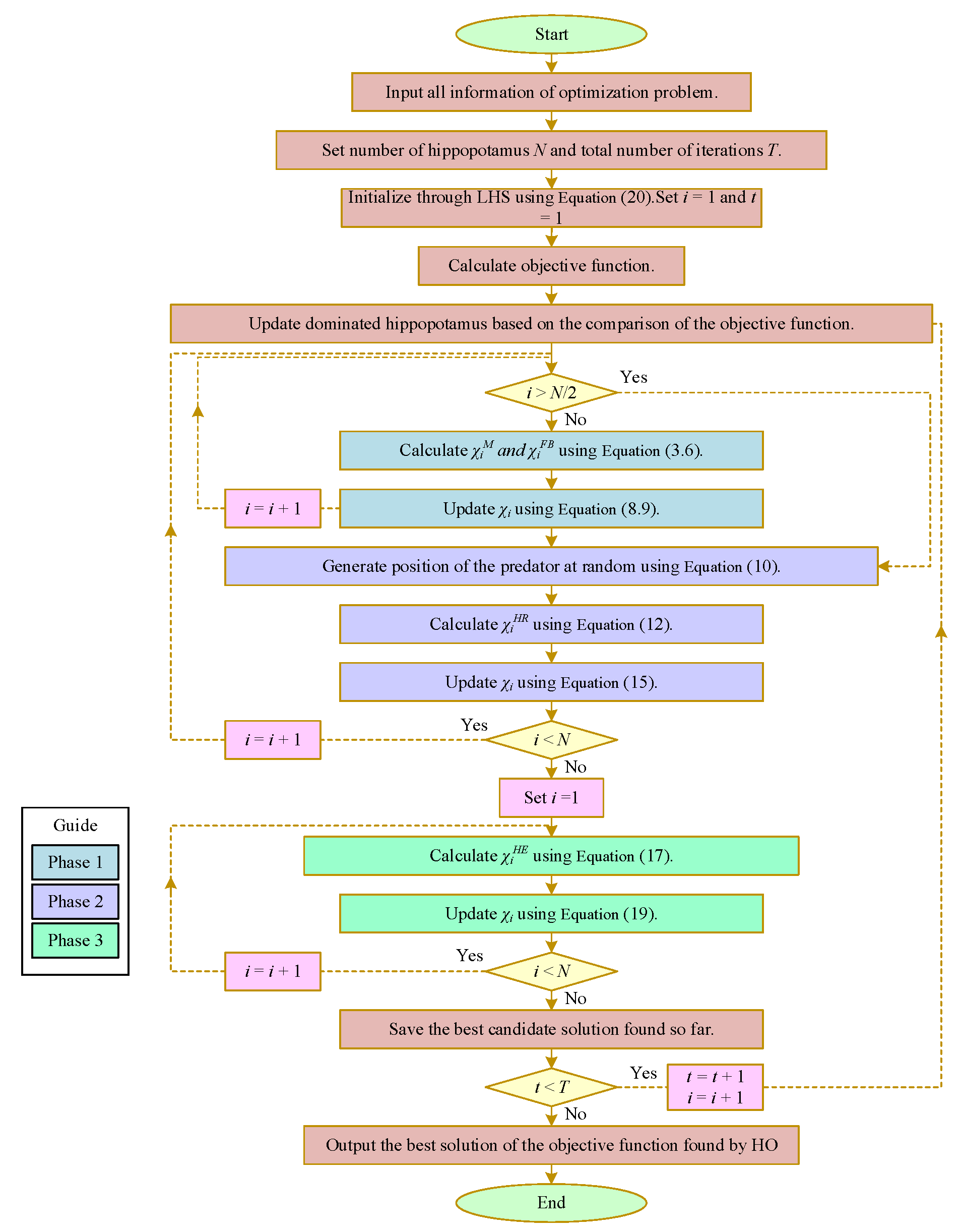
3. Multi-Strategy Improvement HO

Multi-strategy improvement HO uses Latin hypercube sampling instead of random initialization in the initialization stage, which generates a more uniform initial population than random numbers. In the development stage of escaping predators, the Jaya approach of seeking benefits and avoiding harm is adopted, safer locations are constantly approached, and the location of the predator is avoided. In the final selection stage, the population generated by unordered sampling, random crossover, and sequence mutation is compared with the latest generated optimal value to select the result. The HO process diagram is improved on as shown in Figure 2.

Figure 2. Flowchart of IHO.

3.1. Using Latin Hypercube Sampling to Improve Population Diversity

Latin hypercube sampling (LHS) is a method of uniform sampling in a multi-dimensional space, which is used to generate a set of samples that are as uniform as possible and as rarely repeated as possible in each parameter space [21]. The process of Latin hypercube sampling is as follows:

(1)

Divide [0, 1] evenly into n aliquots, and randomly select a point in each interval.

(2)

The position of each sample point is randomly switched to ensure that the sample points on each parameter axis are evenly distributed and not repeated. The HO uses a Latin hypercube drawn evenly distributed from the interval (0, 1)

Sample to initialize the population location, as shown in the following formula:

$$Cootpos\left(i\right)=\left(ub-lb\right)\ast lhs\left(1,D\right)+lb$$

(20)

In this, LHS is based on the Latin hypercubic sampling function, which returns a 1D matrix. The sampling of LHS is more evenly distributed than random. Therefore, the algorithm for population initialization using LHS helps to avoid the population becoming trapped during the initialization phase.

Local optimal solutions improve the global search capability of the algorithm. Moreover, the wider initial distribution of the population also helps the algorithm to explore the favorable regions in the search space faster and improve the efficiency of the algorithm in finding the optimal solution. From Figure 1, using LHS results in more uniform initialization compared to the original algorithm’s random initialization.

To prove this, Figure 3 shows the statistical histogram comparison of random initialization and Latin hypercube sampling initialization, where the number generated is set to 1000. The results show that the distribution of values initialized using LHS is more uniform, and the distribution of histograms is more averaged.

Figure 3. Population distribution map.

3.2. Thoughts on Jaya Seeking Advantages and Avoiding Disadvantages

The Jaya algorithm was proposed by Rao et al. [22] as a new metaheuristic algorithm that utilizes the idea of continuous improvement, Continuously approaching the optimal individual while keeping away from the worst individual, thereby continuously improving the quality of the solution. The Jaya algorithm has fewer control parameters and strong global search ability in comparison with other intelligent optimization algorithms and is widely applied to parameter optimization, scheduling, and other fields. The formula is as follows:

$$h_{m,n,k}^{\prime }=h_{m,n,k}+r_1\left(h_{m,best,k}-\left|h_{m,n,k}\right|\right)-r_2\left(h_{m,worst,k}-\left|h_{m,n,k}\right|\right)$$

(21)

wherein $h_{m,n,k}$ is the value of the $m$ of individual $n$ in the $k$ iteration, $r_1$ and $r_2$ represent two random variables with a value range of [0, 1]; $h_{m,n,k}^{\prime }$ is the value of the $m$ representing the updated individual $n$ in the $k$ iteration; $h_{m,best,k}$ is the $m$ variable value representing the optimal individual in the $k$ iteration; $h_{m,worst,k}$ represents the $m$ variable value of the worst individual in the $k$ iteration.

3.3. Smooth Development Variation

Smooth development variation [23] includes unordered dimensional sampling, random crossover, and sequence mutation. In the fourth stage of the HO algorithm, this article utilizes smooth development mutation to find the minimum value and enhance the convergence efficiency and optimization accuracy of the algorithm.

3.3.1. Random Sampling

Random dimensional sampling can also prevent a decrease in population sparsity and promote vectorization in programming to reduce runtime.

$$rate=ceil\left(\max \left({\displaystyle \frac{t}{\max Iter}},e\right)\right)\times \dim ension$$

(22)

$rate$ is the sampling rate, $\max Iter$ is the maximum iterations, and $\dim ension$ is the dimension of each position vector.

3.3.2. Random Crossover

Random crossover can improve exploration ability by randomly selecting individuals.

$$h_i\left(t+1\right)=h_{r_1}-\left(h_{r_3}-h_{r_2}\right),r_1,r_2,r_3\in rate,and\ne i$$

(23)

where $r_1,r_2,r_3$ are indexes selected randomly.

3.3.3. Sequence Mutation

Random crossover relies on two random individuals. When the radius is too small, it can prematurely fall into local optima. Therefore, we propose sequence mutations to address this issue. Therefore, sequence mutations and random crossover complement each other, improving exploration ability.

$$h_i\left(t+1\right)=\left(h_i\left(t\right)+h_{i-1}\left(t\right)\right)/2$$

(24)

where $h_i\left(t\right)$ is the $i$ individual, $h_{i-1}\left(t\right)$ is the former individual, $h_{i+1}\left(t\right)$ is the new position vector.

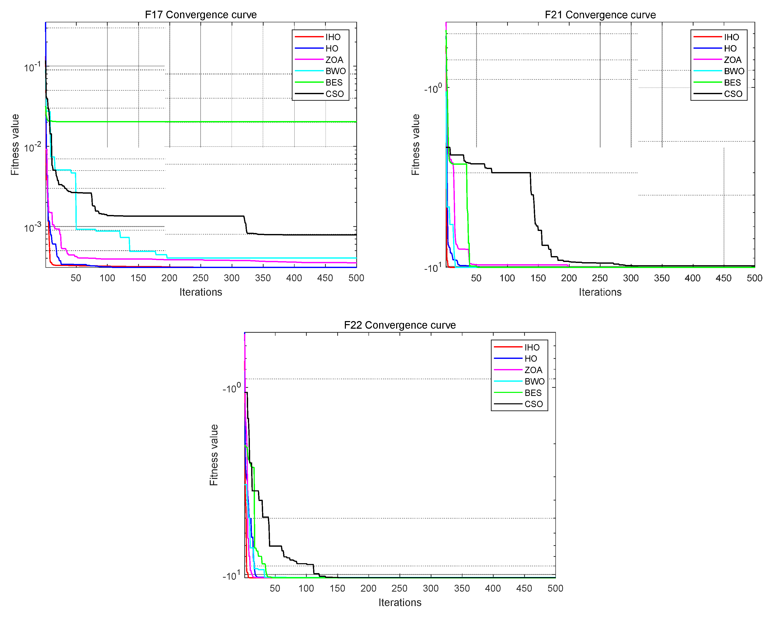
4. Experiments and Results of the Algorithm

Selecting nine functions from the test function for testing, as shown in Table 1, IHO was compared with five optimization algorithms: HO, ZOA [24], CSO [25], BWO [26], and BES [27]. Population size N = 30. The maximum number of iterations is T = 500. The performance of the algorithm is compared with the optimal value (Best), mean (Mean), standard deviation (Std) and convergence curve.

Table 1. Test function.

Function Type	Function	Function Name	Minimum Value
Unimodal testing function	F1	Sphere	0
	F2	Schwefel’s 2.22	0
	F3	Powell Sum	0
Multimodal testing function	F10	Ackley 1	0
	F12	Penalized	0
	F13	Penalized 2	0
Composite Test Function	F17	Branin Function	0.3
	F21	Shekel5	−10
	F22	Shekel7	−10

Figure 4 presents the running results of the six algorithms in nine test functions.

Figure 4. Running results of the six algorithms.

F1, F2, and F3 are unimodal functions used to test the convergence rate of the algorithm and local search ability. Table 2 shows that IHO significantly outperformed the other five optimization algorithms on the unimodal function. For functions F1, F2, and F3, the optimal value and mean value of IHO are also optimal. This shows the excellent local search ability of IHO.

Table 2. Comparison of results in nine test functions.

Function	Indicator	IHO	HO	ZOA	BWO	BES	CSO
F1	Best	0	0	6.79 × 10−257	0.0012855	3.5607 × 10−49	2.0899 × 10−24
	Mean	0	0	5.7194 × 10−248	0.0085168	1.4081 × 10−40	3.3275 × 10−20
	Std	0	0	0	0.009002	4.4204 × 10−40	6.2509 × 10−20
F2	Best	3.8064 × 10−237	4.0835 × 10−196	3.9486 × 10−136	0.021046	5.265 × 10−28	4.5561 × 10−21
	Mean	3.2568 × 10−227	4.0886 × 10−184	3.3091 × 10−131	0.062712	1.526 × 10−26	1.1554 × 10−19
	Std	0	0	7.3205 × 10−131	0.027747	1.4162 × 10−26	1.0822 × 10−19
F3	Best	0	0	5.8723 × 10−170	0.17059	3.2083 × 10−18	789.3893
	Mean	0	0	5.6762 × 10−157	1.9486	3.5527 × 10−9	5458.8957
	Std	0	0	1.7211 × 10−156	2.1075	1.0771 × 10−8	3255.1196
F10	Best	4.4410 × 10−16	4.4410 × 10−16	4.4410 × 10−16	0.0013155	3.9968 × 10−15	9.3157 × 10−12
	Mean	4.4410 × 10−16	4.4410 × 10−16	4.4410 × 10−16	0.0098595	0.066907	3.5665 × 10−11
	Std	0	0	0	0.0057589	0.21158	4.9603 × 10−11
F12	Best	1.5705 × 10−32	1.3134 × 10−6	0.072344	0.00012093	3.3141 × 10−22	0.12557
	Mean	1.5705 × 10−32	0.00059838	0.18427	0.0010186	1.0599 × 10−18	1.8138
	Std	2.885 × 10−482	0.00071235	0.073413	0.00077814	1.6606 × 10−18	4.3809
F13	Best	1.3498 × 10−32	1.2145 × 10−6	1.8168	5.7503 × 10−6	9.0528 × 10−16	1.717
	Mean	1.3498 × 10−32	0.0033994	2.3005	0.00026124	0.071829	7743.1699
	Std	2.885 × 10−481	0.0098188	0.34603	0.00022535	0.062312	12,768.7936
F17	Best	0.39790	0.39790	0.39790	0.39835	0.39789	0.39789
	Mean	0.39790	0.39790	0.39790	0.40044	0.39789	0.39795
	Std	1.6739 × 10−6	3.8556 × 10−10	9.9536 × 10−8	0.0021123	2.005 × 10−8	9.318 × 10−5
F21	Best	−10.1530	−10.1530	−10.1530	−10.1518	−10.1532	−10.0264
	Mean	−10.1530	−10.1530	−10.1528	−10.1321	−7.3826	−8.404
	Std	1.5003 × 10−7	5.7726 × 10−7	0.00071352	0.014468	3.6363	2.4768
F22	Best	−10.4029	−10.4029	−10.4029	−10.3978	−10.4029	−10.394
	Mean	−10.4029	−10.4029	−10.4029	−10.3795	−8.3033	−5.4696
	Std	6.9042 × 10−6	2.1279 × 10−6	8.0885 × 10−5	0.013886	3.3903	3.1227

Multimodal test functions are used to test the performance of the algorithm for solving multimodal complex optimization problems. Specifically, the functions F10, F12, and F13 are multimodal test functions that test the ability of global search and jump out of the local optimal solution. According to the table, IHO has, compared with other algorithms, the best average on F10, F12, and F13 and searches for the smallest optimal value in all three test functions. Especially in F12 and F13, the standard deviation and mean value of IHO are orders of magnitude different from the remaining algorithms. Comparing the optimization results of the algorithm on the multimodal problem shows that IHO has good global search ability and jumps out of the local optimality.

The composite benchmark function is composed of multiple simple functions. Each simple function is a univariate function but is combined to form a composite function of high dimensions. Such functions can test how much algorithms can tolerate unfeasible solutions and their ability to solve large-scale optimization problems. IHO also showed a significant advantage in these three composite functions, with the mean, optimal value, and standard deviation being the lowest among all contrast algorithms.

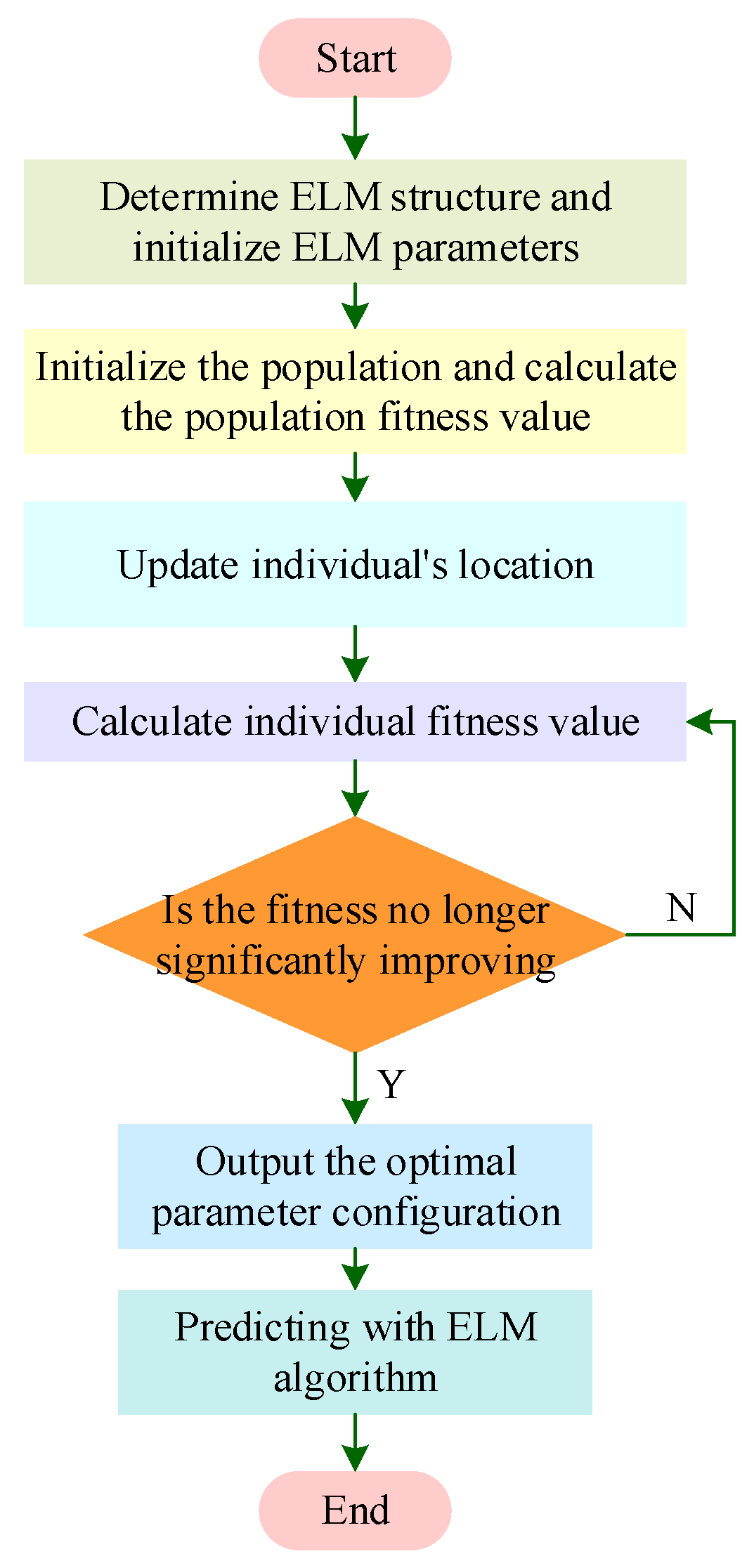
5. Photovoltaic Power Prediction Based on Objective Optimization IHO-ELM

5.1. Extreme Learning Machine (ELM)

The ELM algorithm randomly selects hidden layers and input weight biases, solving the problems of slow learning rate, long iteration time, and the need for manually setting learning parameters in traditional neural networks [28]. Assuming there is a set of training samples $\left(h_i,l_i\right)$, $h_i={\left(h_{i1},h_{i2},\dots ,h_{in}\right)}^T\in R^n$ are input vectors for network samples and $l_i={\left(l_{i1},l_{i2},\dots ,l_{im}\right)}^T\in R^m$ is the output vector of the network. The general form of the standard ELM with L hidden layer neurons is shown in Equation (25).

$$f_L\left(h\right)={\displaystyle \sum _{i=1}^L{\beta }_i{G}_i\left(h\right)={\displaystyle \sum _{i=1}^L{\beta }_i{G}_i\left(a_i,b_i,H\right)}}$$

(25)

In the formula, ${\beta }_i$ are output weights, ${\beta }_i{G}_i\left(a_i,b_i,H\right)$ activates the function, $a_i$ is the input weight of the network, and $b_i$ is the unit threshold for the $i$ hidden layer. However, the connection weights and thresholds between the hidden layer and the input layer of the ELM can affect its prediction accuracy. Therefore, this paper uses the IHO to optimize these two parameters.

The steps to optimize the weight and threshold parameters in the ELM using the IHO optimization algorithm are as follows; the flowchart is shown in Figure 5.

Figure 5. Flowchart of IHO-ELM.

Step 1: Initialize the population and randomly set the initial position and velocity of each individual in the population.

Step 2: Determine fitness and calculate the fitness of each individual.

Step 3: Compare the fitness of each individual with their historical best position and update their position if the historical best position is good.

Step 4: Compare the fitness of the individual in the population with the global optimal position of the population and update its position if the global optimal position is good.

Step 5: Adjust position and speed.

Step 6: If the end condition is met, the position is good enough, or the maximum number of iterations is reached, the above iteration process ends. Otherwise, continue with Step5.

5.2. Example Analysis

To verify the validity of the proposed method, the PV power data from Yulara Solar System 38.3 kW, mono-Si, Roof, 2016, Sails in the Desert-2, from 1 April 23:45 to 6 April 3:35 in 2016, were selected for verification (Data Download|DKA Solar Centre). The sampling interval was 5 min, had a total of 1200 sampling points, and was combined with the corresponding meteorological data, including temperature, radiation, humidity, and other indicators, were combined to form the example data set.

5.3. Evaluation Indicators

MAPE (mean absolute percentage error), MSE (mean square error), MAE (mean absolute error), and RMSE (root mean square error) were selected to evaluate the model prediction accuracy; R² is as follows:

$${\mathrm{e}}_{MAPE}={\displaystyle \frac{1}{n}}{\displaystyle \sum _{i=1}^n\left|\frac{a_i-b_i}{b_i}\right|}\ast 100\%$$

(26)

$${\mathrm{e}}_{MAE}={\displaystyle \frac{1}{\mathrm{n}}}{\displaystyle \sum _{i=1}^{\mathrm{n}}\left|a_i-b_i\right|}$$

(27)

$${\mathrm{e}}_{RMSE}=\sqrt{{\displaystyle \frac{1}{\mathrm{n}}}{\displaystyle \sum _{i=1}^n{\left(a_i-b_i\right)}^2}}$$

(28)

$$R^2=1-\left(RSS/TSS\right)$$

(29)

$$e_{MSE}={\displaystyle \frac{1}{n}}{{\displaystyle \sum }}_{i=1}^n{\left(a_i-b_i\right)}^2$$

(30)

where $a_i$ is the predicted value of PV power at the $i_{th}$ prediction point; $b_i$ is the true value of PV power at the $i_{th}$ prediction point; Total Sum of Squares(TSS) is the variance of the true value y, Residual Sum of Squares(RSS); the value range of the determination coefficient of R² is [0, 1]. The closer the value is to 1, the more the data variance is explained by the model and the better the performance.

5.4. Results and Discussion

Before making a prediction, first normalize the sample data, as shown in Equation (31):

$$x^{\prime }={\displaystyle \frac{x_i-x_{\min } }{x_{\max }-x_{\min }}}$$

(31)

wherein $x^{\prime }$ is the normalized value, $x_i$ is the normalized raw data required, $x_{\max }$ and $x_{\min }$ is the maximum and minimum of the raw value, respectively.

The IHO-ELM can be used to predict the power flow chart, as shown in Figure 6.

Figure 6. Flowchart of IHO-ELM prediction.

The computational efficiency of optimization algorithms can usually be evaluated for their performance. So, this article first analyzes the efficiency of algorithms. When optimizing the connection weights and thresholds of the ELM model, set the value of the optimization algorithm population to 20 and set the maximum number of iterations to 150. The fitness values of the IHO algorithm proposed in this paper were compared with those of the HO algorithm and CSO algorithm; the results are shown in Figure 7.

Figure 7. Iteration curves of three models.

According to Figure 7, the CSO algorithm converges at 94 iterations with a fitness of approximately 0.013988; The HO algorithm converges after approximately 68 iterations with a fitness of approximately 0.0044711; The IHO algorithm proposed in this article converges with a fitness of approximately 0.003473 after approximately 26 iterations. The IHO algorithm has a faster convergence speed and stronger optimization ability, which can increase the probability of jumping out of local optimal solutions, finding better solutions, and improving computational efficiency.

Secondly, to assess the performance of the model presented in this paper, we compared it with the three models from the two perspectives of optimization algorithm and single model. In terms of a single model, an ELM single model is selected for comparison. In terms of optimization algorithms, a comparison was made between the CSO-optimized ELM and the unimproved HO algorithm-optimized ELM. The comparison results are presented in Table 3 and Table 4.

Table 3. Prediction error results of 8 models.

Prediction Model	MAE	MAPE	MSE	RMSE	R2
IHO-ELM	0.04760	0.11662	0.00376	0.06129	0.99998
HO-ELM	0.06164	0.14158	0.00611	0.07819	0.99996
CSO-ELM	0.11791	0.12216	0.03314	0.18203	0.99979
ELM	0.23916	0.31099	0.10427	0.32291	0.99934
LSTM	0.43945	0.33520	0.39491	0.62842	0.99750
TCN	0.27854	0.66627	0.39963	0.63216	0.99747
BP	0.90367	0.86687	1.83062	1.35310	0.98843
SVM	1	1.30972	1.89581	1.37690	0.98801

Table 4. The two optimal models predict the error results.

Prediction Model	MAE	MAPE	MSE	RMSE
IHO-ELM	0.04760	0.11662	0.00376	0.06129
HO-ELM	0.06164	0.14158	0.00611	0.07819
Percentage reduction in error	22.78%	17.62%	38.5%	21.61%

Table 3 shows the performance of different comparison models, and the results are analyzed as follows:

(1)

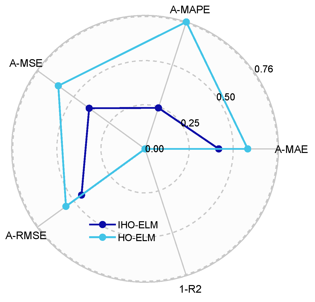
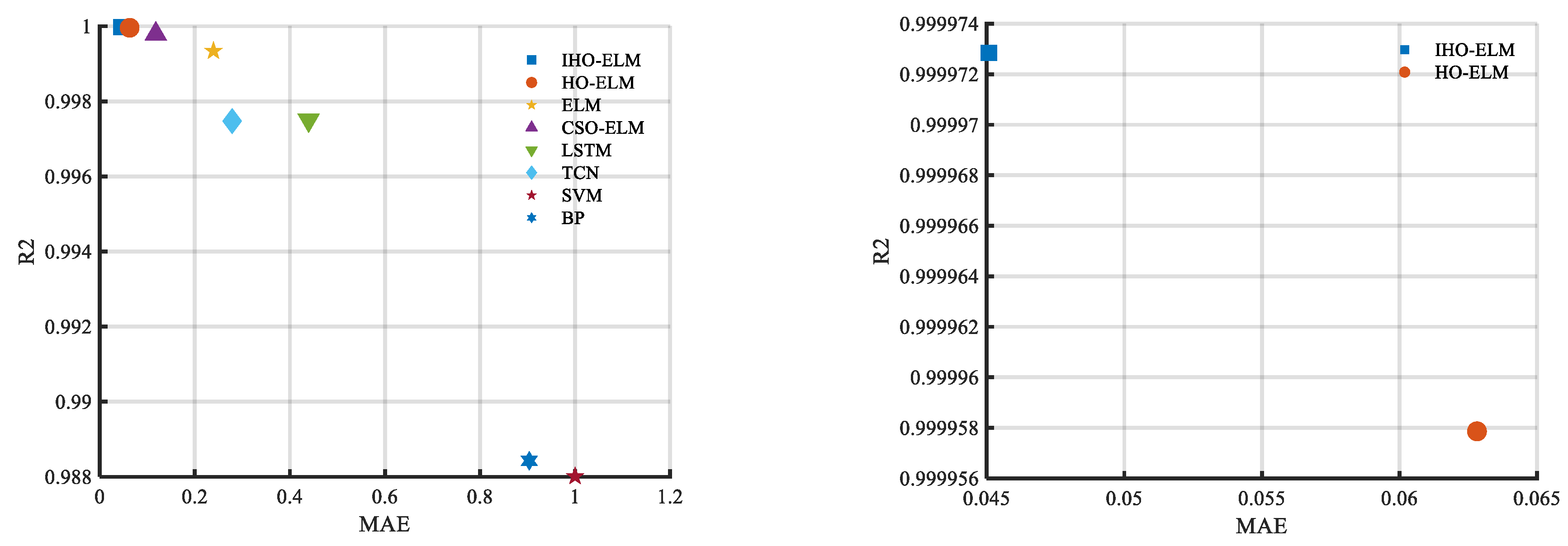
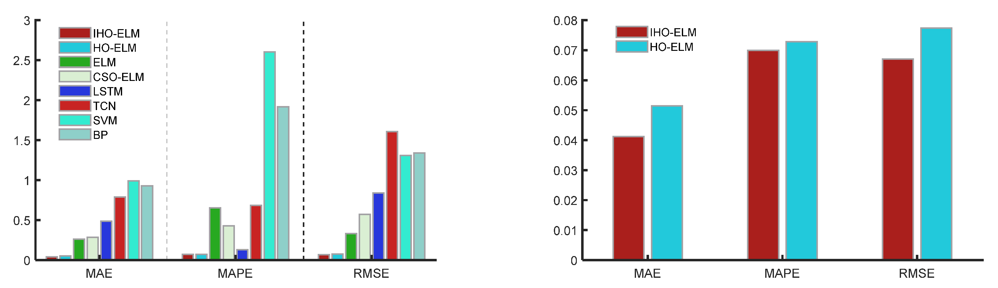
Compared with the ELM, CSO-ELM, and HO-ELM, the IHO-ELM prediction model achieved the best accuracy, with MAPE, RMSE, MAE, and MSE values being 11.6626%, 0.06129, 0.047593, and 0.0037564.

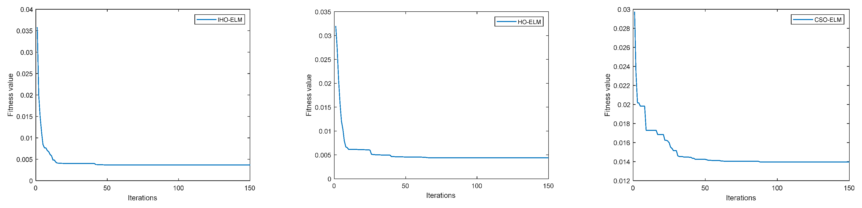
(2)

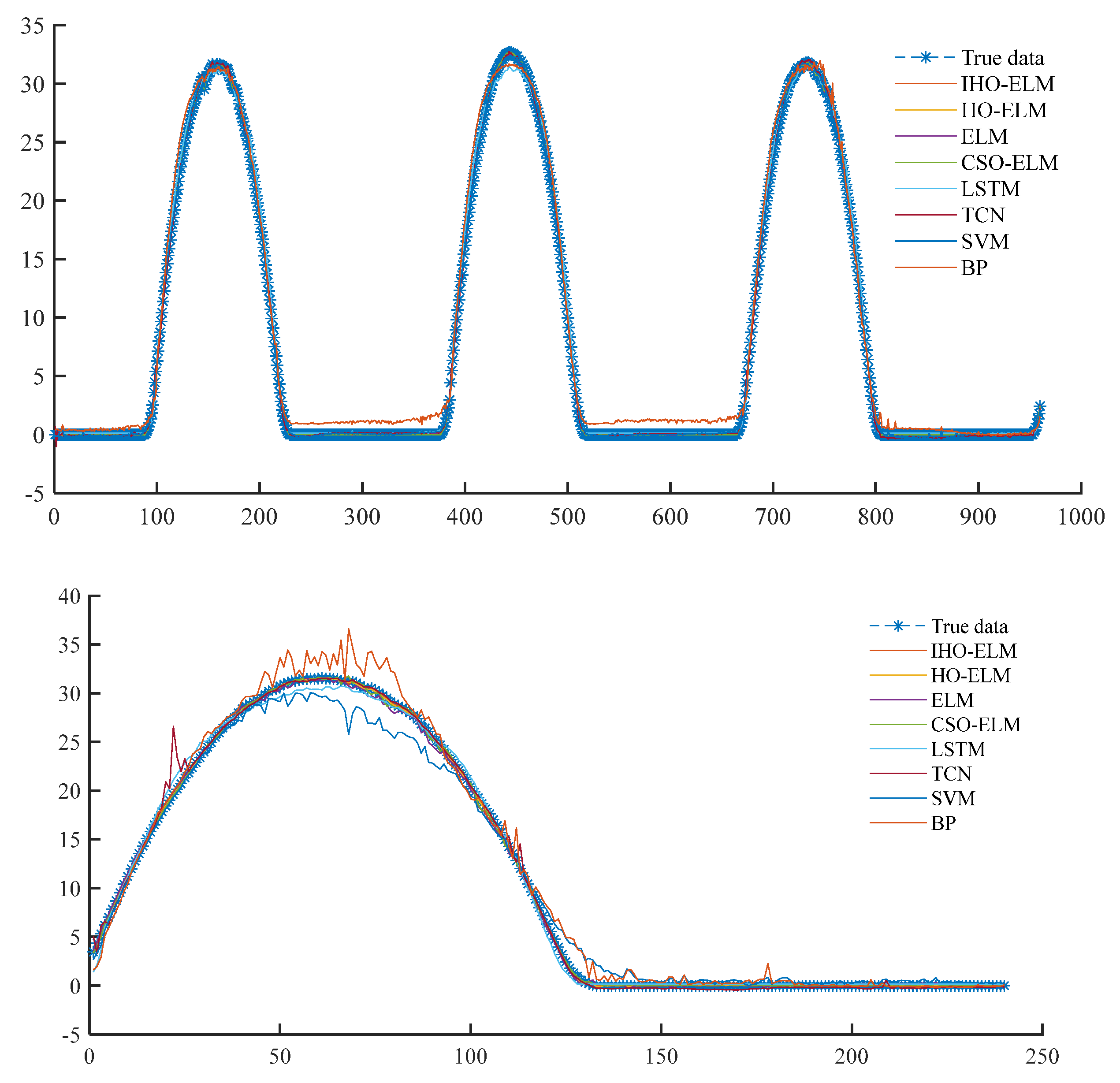
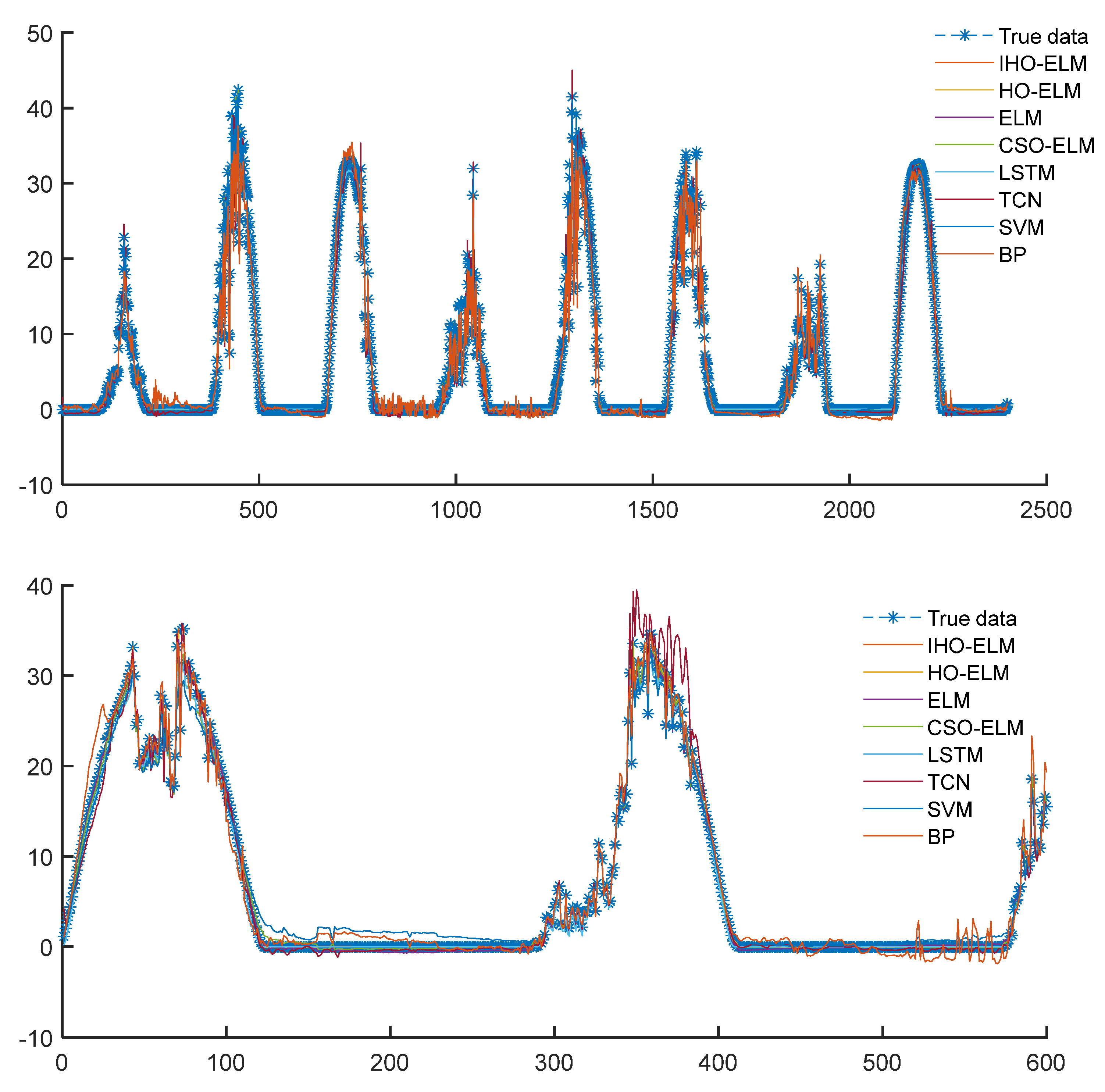
From Figure 8, Figure 9, Figure 10 and Figure 11, the accuracy of the ELM model using optimization methods is significantly higher than that of a single optimized ELM model without using optimization methods, indicating the necessity of connecting the weights and thresholds of the optimized ELM model.

Figure 8. Radar chart of IHO-ELM and HO-ELM evaluation index results.

Figure 9. Bar chart of evaluation indicators for eight prediction models.

Figure 10. Scatter plot of evaluation indicators for eight prediction models.

Figure 11. Curve plots of 8 models’ PV Power training and prediction sets.

(3)

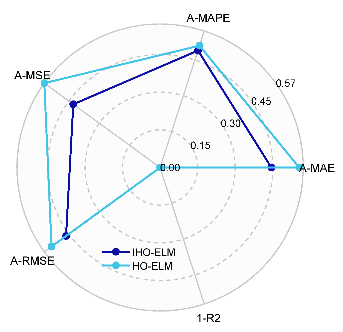
The optimized model has better accuracy than the unoptimized model and the traditional CSO-optimized model. The MAPE, RMSE, MAE, and MSE indicators of the IHO-ELM were reduced by 17.62%, 21.61%, 22.78%, and 38.5%, respectively, compared to the HO-ELM from Table 4, significantly better than the unimproved HO optimization model.

5.5. Further Analysis

To further validate the performance and generalization ability of the proposed model in improving prediction accuracy. Select other PV power data from Yulara 3 mono-Si Roof 2016 Sails in the Desert—3|DKA Solar Centre, on 1 July 00:00–11 July 9:55 in 2016. Sampling was conducted every 15 min, resulting in a total of 3000 sampling points. Select the top 80% of the data as the training set and the bottom 20% of the data as the testing set. The decomposition steps and experimental environment are the same as above, and the results obtained are shown in Table 5 and Table 6. The predicted results can be more intuitively presented in Figure 12, Figure 13, Figure 14 and Figure 15.

Table 5. 8 models’ prediction error results.

Prediction Model	MAE	MAPE	MSE	RMSE	R2
IHO-ELM	0.04121	0.69879	0.00449	0.06697	0.99996
HO-ELM	0.05150	0.72837	0.00598	0.07733	0.99995
CSO-ELM	0.06093	1.00370	0.00759	0.08713	0.99993
ELM	0.26328	6.52800	0.10918	0.33043	0.99901
LSTM	0.48613	1.28880	0.70688	0.84076	0.99359
TCN	0.79034	6.85980	2.58130	1.60660	0.97658
SVM	0.99275	26.0436	1.71340	1.30900	0.98445
BP	0.92858	19.1984	1.79300	1.33900	0.98370

Table 6. The two optimal models’ PV predict the error results.

Prediction Model	MAE	MAPE	MSE	RMSE
IHO-ELM	0.04121	0.69879	0.00449	0.06697
HO-ELM	0.05150	0.72837	0.00598	0.07733
Percentage reduction in error	19.9%	4.1%	25%	13.4%

Figure 12. Radar chart of PV prediction evaluation index results.

Figure 13. Bar chart of PV prediction evaluation index results.

Figure 14. Scatter plot of PV prediction evaluation index results.

Figure 15. Curve plots of 8 models’ PV training and prediction sets.

According to Table 5, the proposed models MAE, MAPE, MSE, and RMSE are 0.041205, 0.69879, 0.0044853, and 0.066973, respectively, which are still superior to other benchmark models. Compared to the HO-ELM, they have increased by 19.9%, 4.1%, 25%, and 13.4%, respectively. The IHO algorithm proposed in this article can improve the prediction accuracy and has good optimization accuracy.

6. Conclusions

This paper presents a hybrid Improved Hippopotamus Optimization algorithm that effectively enhances global search and convergence efficiency by integrating Latin hypercube sampling, Jaya’s optimization principles, unordered dimension sampling, random crossover, and sequential mutation. The IHO algorithm demonstrates superior optimization accuracy, speed, and stability, compared to HO and four other algorithms across nine test functions. When applied to the extreme learning machine model, IHO significantly improves prediction accuracy for solar photovoltaic power generation, outperforming seven other prediction models. Further validation in a different region confirms the IHO-ELM model’s enhanced prediction accuracy and generalization capability. Future work will focus on integrating decomposition denoising techniques with updated optimization models to further refine prediction accuracy.

References

- Boussaïd, I.; Lepagnot, J.; Siarry, P. A survey on optimization metaheuristics. Inf. Sci. 2013, 237, 82–117. [Google Scholar] [CrossRef]
- Tang, J.; Liu, G.; Pan, Q. A review on representative swarm intelligence algorithms for solving optimization problems: Applications and trends. IEEE/CAA J. Autom. Sin. 2021, 8, 1627–1643. [Google Scholar] [CrossRef]
- Aslan, M.F.; Durdu, A.; Sabanci, K. Goal distance-based UAV path planning approach, path optimization and learning-based path estimation: GDRRT*, PSO-GDRRT* and BiLSTM-PSO-GDRRT. Appl. Soft Comput. 2023, 137, 110156. [Google Scholar] [CrossRef]
- Lu, Z.; Whalen, I.; Dhebar, Y.; Deb, K.; Goodman, E.D.; Banzhaf, W.; Boddeti, V.N. Multiobjective evolutionary design of deep convolutional neural networks for image classification. IEEE Trans. Evol. Comput. 2020, 25, 277–291. [Google Scholar] [CrossRef]
- Hu, H.; Lei, W.; Gao, X.; Zhang, Y. Job-shop scheduling problem based on improved cuckoo search algorithm. Int. J. Simul. Model 2018, 17, 337–346. [Google Scholar] [CrossRef]
- Kennedy, J.; Eberhart, R. Particle swarm optimization. In Proceedings of the ICNN’95-International Conference on Neural Networks, Perth, WA, Australia, 27 November–1 December 1995; pp. 1942–1948. [Google Scholar]
- Mirjalili, S.; Lewis, A. The whale optimization algorithm. Adv. Eng. Softw. 2016, 95, 51–67. [Google Scholar] [CrossRef]
- Arora, S.; Singh, S. Butterfly optimization algorithm: A novel approach for global optimization. Soft Comput. 2019, 23, 715–734. [Google Scholar] [CrossRef]
- Heidari, A.A.; Mirjalili, S.; Faris, H.; Aljarah, I.; Mafarja, M.; Chen, H. Harris hawks optimization: Algorithm and applications. Future Gener. Comput. Syst. 2019, 97, 849–872. [Google Scholar] [CrossRef]
- Zhao, W.; Wang, L.; Zhang, Z. Artificial ecosystem-based optimization: A novel nature-inspired meta-heuristic algorithm. Neural Comput. Appl. 2020, 32, 9383–9425. [Google Scholar] [CrossRef]
- Abdollahzadeh, B.; Gharehchopogh, F.S.; Mirjalili, S. African vultures optimization algorithm: A new nature-inspired metaheuristic algorithm for global optimization problems. Comput. Ind. Eng. 2021, 158, 107408. [Google Scholar] [CrossRef]
- Amiri, M.H.; Mehrabi Hashjin, N.; Montazeri, M.; Mirjalili, S.; Khodadadi, N. Hippopotamus optimization algorithm: A novel nature-inspired optimization algorithm. Sci. Rep. 2024, 14, 5032. [Google Scholar] [CrossRef]
- Zhang, Z.; Xu, W.; Gong, Q. Short-Term Load Forecasting Based on TLBGA-GRU Neural Network. Comput. Eng. 2022, 48, 69–76. [Google Scholar]
- Han, J.; Yan, L.; Li, Z. LfEdNet: A Task-based Day-ahead Load Forecasting Model for Stochastic Economic Dispatch. arXiv 2020, arXiv:2008.07025. [Google Scholar]
- Akhtar, S.; Shahzad, S.; Zaheer, A.; Ullah, H.S.; Kilic, H.; Gono, R.; Jasiński, M.; Leonowicz, Z. Short-term load forecasting models: A review of challenges, progress, and the road ahead. Energies 2023, 16, 4060. [Google Scholar] [CrossRef]
- Acquah, M.A.; Jin, Y.; Oh, B.-C.; Son, Y.-G.; Kim, S.-Y. Spatiotemporal Sequence-to-Sequence Clustering for Electric Load Forecasting. IEEE Access 2023, 11, 5850–5863. [Google Scholar] [CrossRef]
- Yan, H.; Yu, X.; Li, D.; Xiang, Y.; Chen, J.; Lin, Z.; Shen, J. Research on commercial sector electricity load model based on exponential smoothing method. In International Conference on Adaptive and Intelligent Systems; Springer: Berlin/Heidelberg, Germany, 2022; pp. 189–205. [Google Scholar]
- Liang, Z.; Chengyuan, Z.; Zhengang, Z.; Dacheng, Z. Short-term load forecasting based on kalman filter and nonlinear autoregressive neural network. In Proceedings of the 2021 33rd Chinese Control and Decision Conference (CCDC), Kunming, China, 22–24 May 2021; pp. 3747–3751. [Google Scholar]
- Bian, H.; Wang, Q.; Xu, G.; Zhao, X. Research on short-term load forecasting based on accumulated temperature effect and improved temporal convolutional network. Energy Rep. 2022, 8, 1482–1491. [Google Scholar] [CrossRef]
- Huang, G.-B.; Zhu, Q.-Y.; Siew, C.-K. Extreme learning machine: A new learning scheme of feedforward neural networks. In Proceedings of the 2004 IEEE International Joint Conference on Neural Networks (IEEE Cat. No. 04CH37541), Budapest, Hungary, 25–29 July 2004; pp. 985–990. [Google Scholar]
- Loh, W.-L. On Latin hypercube sampling. Ann. Stat. 1996, 24, 2058–2080. [Google Scholar] [CrossRef]
- Rao, R. Jaya: A simple and new optimization algorithm for solving constrained and unconstrained optimization problems. Int. J. Ind. Eng. Comput. 2016, 7, 19–34. [Google Scholar]
- Wu, L.; Chen, E.; Guo, Q.; Xu, D.; Xiao, W.; Guo, J.; Zhang, M. Smooth Exploration System: A novel ease-of-use and specialized module for improving exploration of whale optimization algorithm. Knowl.-Based Syst. 2023, 272, 110580. [Google Scholar] [CrossRef]
- Trojovská, E.; Dehghani, M.; Trojovský, P. Zebra optimization algorithm: A new bio-inspired optimization algorithm for solving optimization algorithm. IEEE Access 2022, 10, 49445–49473. [Google Scholar] [CrossRef]
- Meng, X.; Liu, Y.; Gao, X.; Zhang, H. A new bio-inspired algorithm: Chicken swarm optimization. In Advances in Swarm Intelligence, Proceedings of the 5th International Conference, ICSI 2014, Hefei, China, 17–20 October 2014; Part I 5; Springer: Berlin/Heidelberg, Germany, 2014; pp. 86–94. [Google Scholar]
- Zhong, C.; Li, G.; Meng, Z. Beluga whale optimization: A novel nature-inspired metaheuristic algorithm. Knowl.-Based Syst. 2022, 251, 109215. [Google Scholar] [CrossRef]
- Alsattar, H.A.; Zaidan, A.; Zaidan, B. Novel meta-heuristic bald eagle search optimisation algorithm. Artif. Intell. Rev. 2020, 53, 2237–2264. [Google Scholar] [CrossRef]
- Wang, Y.; Wang, W. Research on E-commerce GMV prediction based on LSTM-RELM combination model. Comput. Eng. Appl. 2023, 59, 321–327. [Google Scholar]
Disclaimer/Publisher’s Note: The statements, opinions and data contained in all publications are solely those of the individual author(s) and contributor(s) and not of MDPI and/or the editor(s). MDPI and/or the editor(s) disclaim responsibility for any injury to people or property resulting from any ideas, methods, instructions or products referred to in the content. |
© 2024 by the authors. Licensee MDPI, Basel, Switzerland. This article is an open access article distributed under the terms and conditions of the Creative Commons Attribution (CC BY) license (https://creativecommons.org/licenses/by/4.0/).