Reinforcement-Learning-Based Path Planning: A Reward Function Strategy

Abstract

Path planning is a fundamental task for autonomous mobile robots (AMRs). Classic approaches provide an analytical solution by searching for the trajectory with the shortest distance; however, reinforcement learning (RL) techniques have been proven to be effective in solving these problems with the experiences gained by agents in real time. This study proposes a reward function that motivates an agent to select the shortest path with fewer turns. The solution to the RL technique is obtained via dynamic programming and Deep Q-Learning methods. In addition, a path-tracking control design is proposed based on the Lyapunov candidate function. The results indicate that RL algorithms show superior performance compared to classic A* algorithms. The number of turns is reduced by 50%, resulting in a decrease in the total distance ranging from 3.2% to 36%.

1. Introduction

Trajectory planning in autonomous mobile robots (AMRs) has been a subject of study for some time. Its importance lies in the need to reduce the time and energy costs of a robot’s trajectory. In robotic systems, path planning corresponds to the connection between environmental information and motion control [1]. Several techniques have been developed that allow a robot to go from point $P_1$ to point $P_2$, corresponding to the position of an object [2]. During path planning, it is essential to avoid static or dynamic obstacles. In recent years, different approaches have been developed with the objective of integrating environmental variables as well as the movement dynamics of AMRs [3,4,5].

Path planning is the key to success in mobile robotic systems. Any path-planning technique can provide a satisfactory result, even if it is not the optimal path. Numerous algorithms aim to minimize path cost by considering the distance factor; however, there are other variables, such as time complexity and search area, considered in the optimization of these algorithms [3].

The most common classic approaches used in route planning are the following: cell decomposition (CD), which establishes the path between the start and end points through the discretization of the environment into small portions called cells, using algorithms based on graphs such as the Dijkstra and A* algorithms [6]; the roadmap approach (RA), which establishes connections between the vertices of each object through a line called the edge line, as long as there is no overlap with the objects and the line [7]; the artificial potential field (APF), which considers an attractive force between the starting point and the target point, while the objects generate repulsive forces [8]; and the rapidly exploring random tree (RRT), which bases its operation on fast sampling that allows the starting point to be expanded until the tree is close enough to the target point [9]. In addition to these techniques, numerous algorithms based on intelligent systems, such as those of logic and diffusion, have been developed, including neural networks (NNs) and genetic algorithms (GAs). The selection of the technique to be applied is mainly based on the available information about the environment [2,4,5,10,11].

Cell decomposition methods can be used in global path planning and local path planning. They mainly focus on discretizing free space into cells and selecting the path through a sequence of cells. The set of solutions involving classical techniques can be represented on mathematical graphs with acceptable accuracy; therefore, the incorporation of artificial intelligence (AI) and automated reasoning has gained popularity, with the aim of incorporating multiple variables. These variables include environmental variables or variables that influence the dynamics of a robot, such as the incorporation of holonomic constraints [3,12].

RL is an algorithm that aims to find an optimal behavior strategy for an agent when interacting with an unknown environment. The agent receives positive, negative, or null reward signals for actions performed, and the computed strategy should maximize the accumulated rewards. The agent explores an environment to quickly learn about actions with significant rewards. This definition includes a wide range of problems, from sequential decision-making control to games and situations involving social dilemmas. It has applications for control engineering, operative investigation, and machine learning [13,14,15].

Multiple studies have demonstrated that RL algorithms are capable of estimating the optimal trajectory from the initial point to the target point in dynamic and static environments [16,17,18]; however, there are limitations, such as the high consumption of computational resources for large environments, which represents a higher consumption of memory related to the $Q$ value chart. In addition, the increase in cells drastically reduces the convergence rate [19,20,21].

Relevant studies have demonstrated acceptable results; ref. [22] introduced a mobile virtual objective that increases the low learning rate of the classical Q-Learning algorithm by incorporating distance as a metric. An alternative to improving the performance of the algorithm is to update the reward function, as carried out in [23]. The space-state and action-state tables are also sometimes modified, considering the total knowledge of the environment as well as static obstacles. On the other hand, the initialization of the $Q$ value table accelerates the learning process [24].

Similarly, the dynamic modification of $Q$ values based on the knowledge of the distance between the agent and the obstacles enhances the performance of the classic Q-Learning algorithm regarding time and distance [21]. Therefore, the assignment of rewards for each state increases performance over the classical path-planning algorithms, which are A* and RRT [25].

Another improvement is the integration of factors such as the computational time, length of trajectory, collision rate, and success rate to improve the efficiency of obstacle avoidance in dynamic environments.

ACO algorithms are used to achieve smooth trajectories in dynamic environments, taking into account cinematic restrictions, trajectory length, and path-smoothing constraint [26]. GAs show satisfactory results for smoothing trajectories and for generating diverse trajectories [27].

The contributions of this study focus on the following:

• A reward function capable of finding a trade-off between trajectory distance and time when minimizing the number of turns.
• A neural network architecture to extract the optimal trajectory according to the proposed approach employing the Deep Q-Learning technique.
• A trajectory-tracking controller design based on Lyapunov’s stability criteria.

To evaluate the algorithm’s performance in terms of execution time, memory use, and computational resources, it is compared to two RL algorithms.

The remainder of this study is divided as follows: Section 2 discusses the proposed methodology, RL algorithms, and the design of the trajectory-tracking controller, while Section 3 presents a summary of the results obtained.

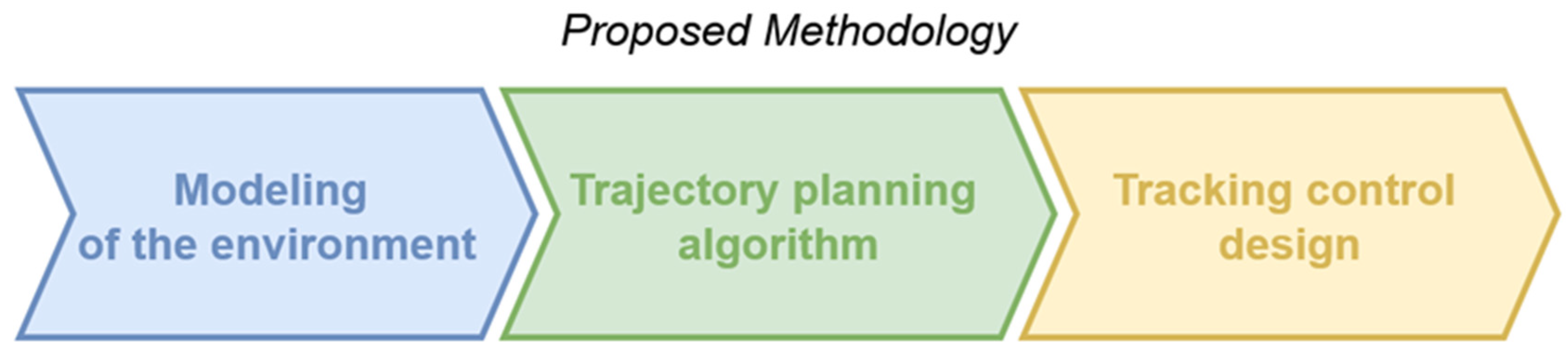
2. Proposed Methodology

The robot navigation problem can be divided into three subtasks: environment modeling, a trajectory-planning algorithm, and tracking control design. Figure 1 shows the proposed methodology. Environment modeling is considered a cell decomposition technique with uniformly sized cells and static as well as dynamic obstacles. The proposed path-planning algorithm is based on the Markov decision process (MDP), with two different solution approaches: a tabular technique and neural networks. Both algorithms aim to motivate an agent to take shorter routes with fewer turns. The design of the tracking control is founded on Lyapunov’s stability criteria. The proposed candidate function is the root mean square.

Figure 1. Proposed methodology.

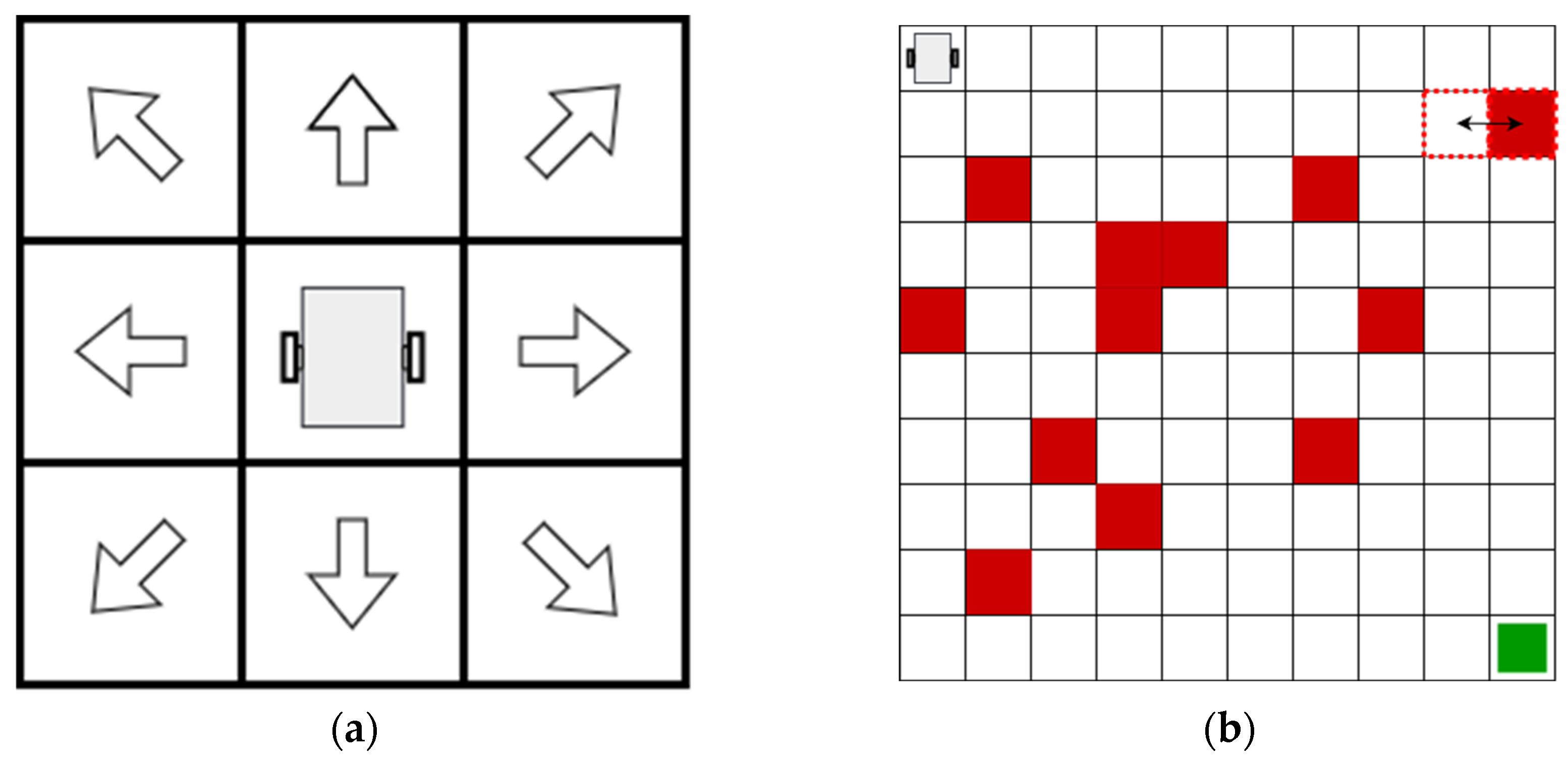
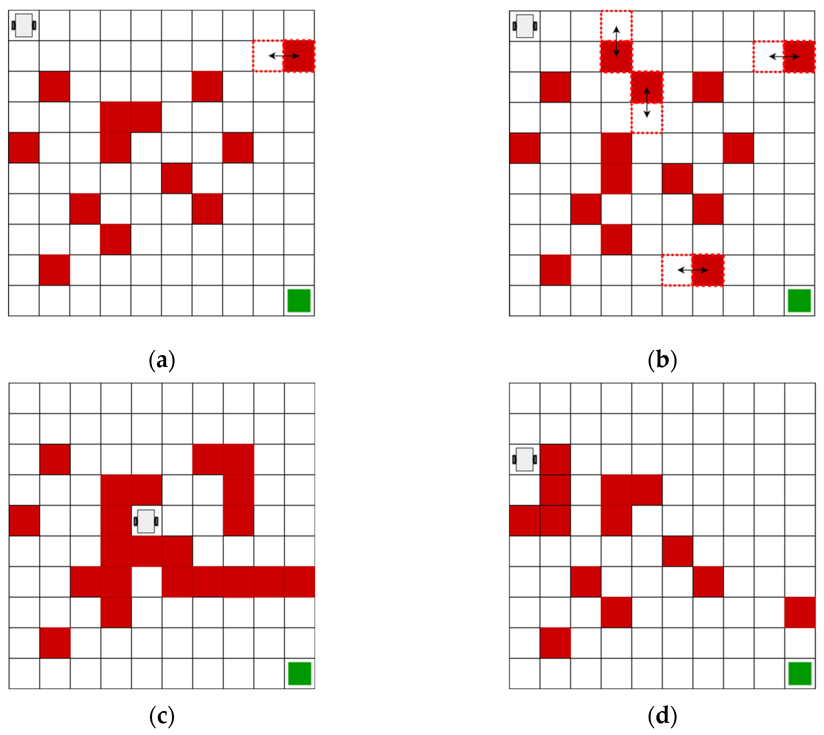
2.1. Environment Modeling

In this study, an AMR was modeled with differential traction to maneuver and avoid collisions with dynamic as well as static obstacles. An environment was created based on the cell decomposition technique, since it facilitates the development of the RL algorithm by converting the problem into a finite state. Each cell represents the orientation, position, and any other possible state according to the problem to be resolved.

In the environment, the robot is considered a punctual mass with a radius smaller than the cell size, so 8 actions are allowed for each state: forward, backward, left, right, forward–left, forward–right, backward–left, and backward–right, as shown in Figure 2a. In this method, obstacles are modeled in such a manner that if the border of an obstacle partially overlaps a cell, the entire cell will be considered an obstacle.

Figure 2. Diagram of the environment and allowed actions for each state. (a) Allowed actions for the robot. (b) Cell decomposition techniques for the model proposed.

The environments used have a dimension of $10\times 10$ cells, and only the positions of the obstacles vary. Figure 2b shows an example of the environment. The red-filled cells represent the obstacles, the red-dotted cells represent the area where an obstacle has motion for each interaction, and the target point is represented in green. The robot is located at position $0, 0$ and the target at $9, 9$. Each cell represents an $x,y$ coordinate in integers.

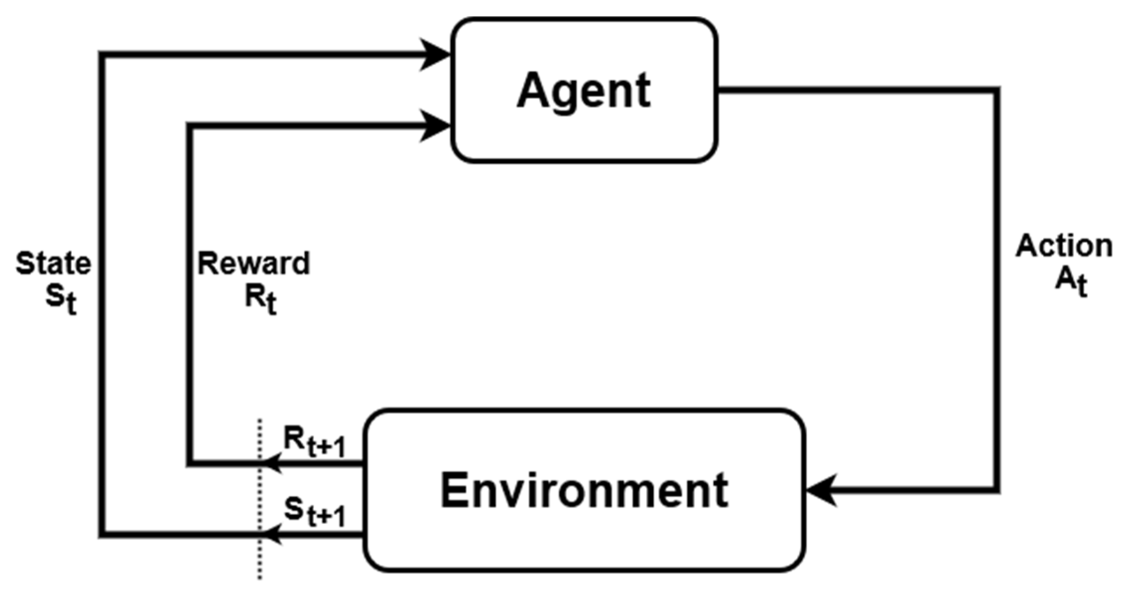
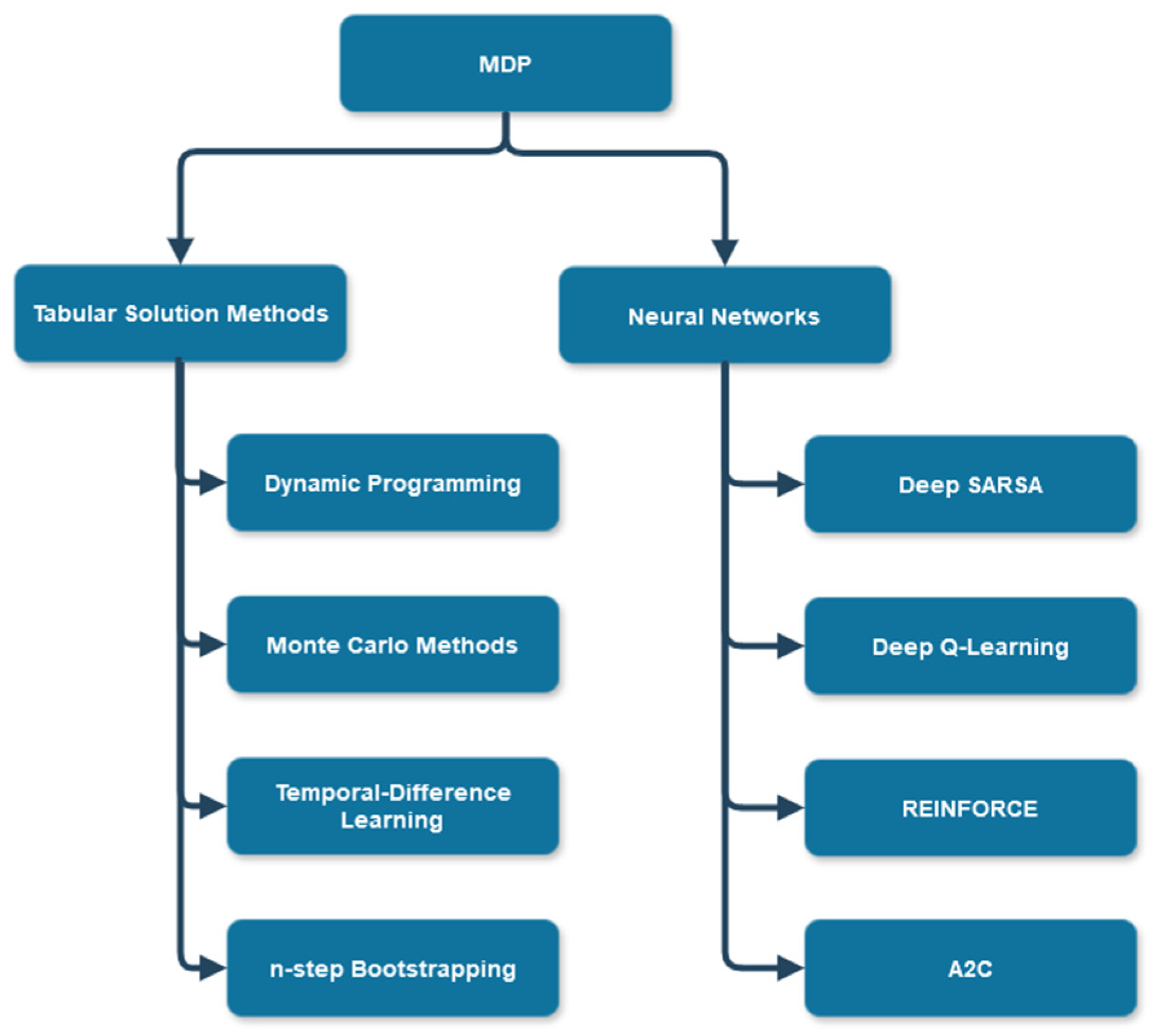
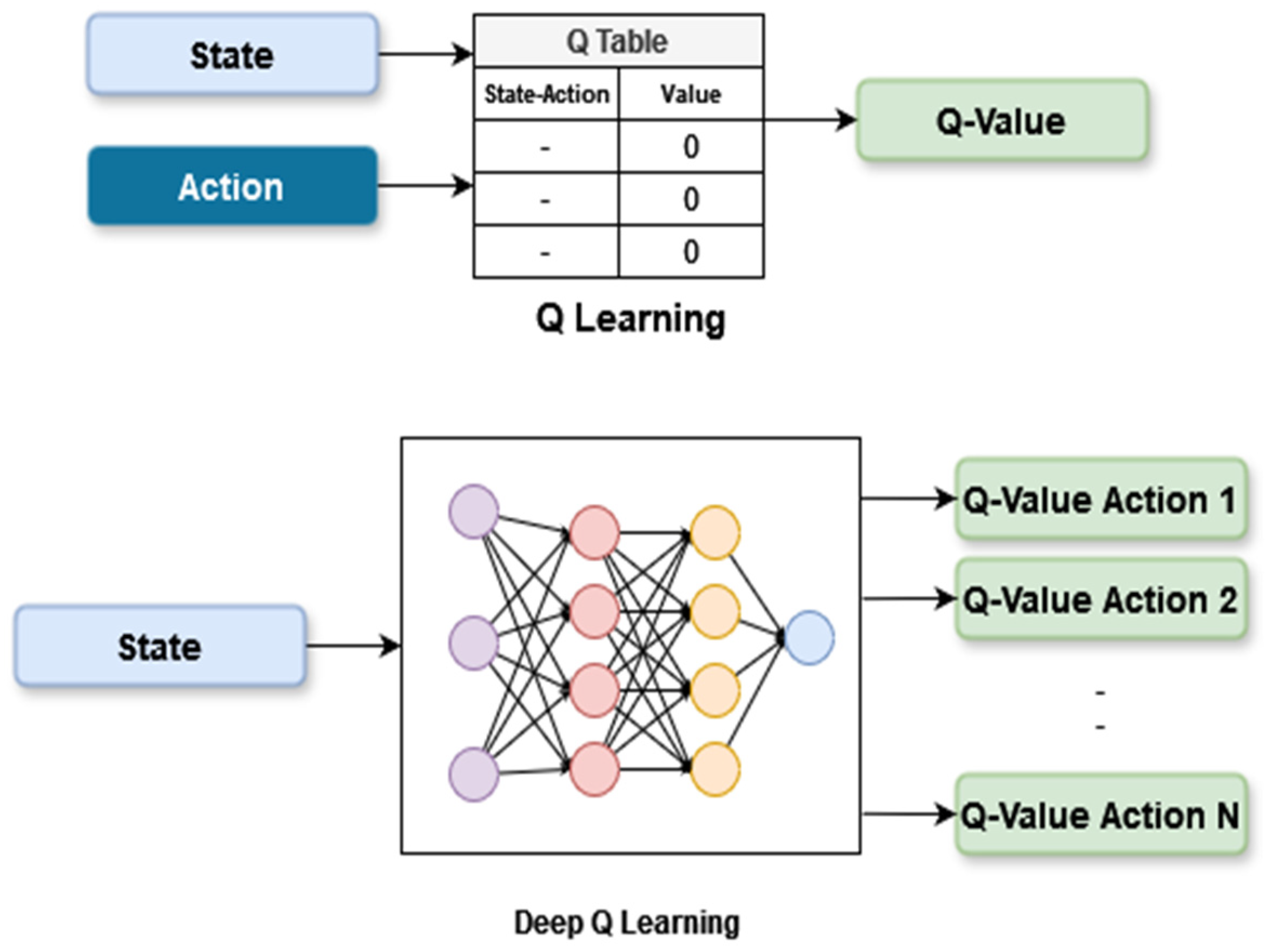
2.2. Reinforcement Learning and Q-Learning Algorithm

The sequence of decisions in RL is determined by the Markov decision process introduced by Bellman [28]. The MDP consists of a set of states of an environment, a set of actions taken by an agent, and a transition probability distribution that gives the probability of moving from one state to another after completing an action in another state. This process captures the effect of each action that has an associated trade-off.

Figure 3 shows the process of RL in which the following elements interact [15,29]:

Figure 3. The agent–environment interaction in a Markov decision process [15].

• An agent is an entity that perceives/explores an environment and makes decisions.
• An environment includes everything surrounding an agent and is generally assumed to be stochastic.
• Actions correspond to an agent’s movement in an environment.
• State is the representation of an agent over time.
• Reward is a numerical value that an agent tries to maximize by the selection of its actions.
• Policy represents a strategy used by an agent to select an action based on the present state.

The following is a general presentation of the MDP, extracted from [14,15].

The result of the MDP corresponds to a sequence or trajectory of the groups of states, $S_t$, actions, $A_t$, and rewards, $R_t$, for each instant of time, $t=0, 1, 2, 3\dots$. The beginning of the sequence starts as shown in Equation (1):

$$S_0,A_0,R_1,S_1,A_1,R_2,S_2,A_2,R_3,\dots$$

(1)

The selection process for a subsequent state must comply with the fact that the next state will depend on the immediately preceding state and action, and not on any other previous states or actions. Furthermore, all possible states must have a probability greater than $0$, which guarantees that all actions are eligible at time $t$. The probability of the occurrence of these states is represented in Equation (2):

$$p\left(s^{\prime },r|s,a\right)\stackrel{·}{=}\mathrm{Pr}\left\{S_t=s^{\prime }, { R}_t=r \right| S_{t-1}=s, A_{t-1}=a\}$$

(2)

where $p$ defines the dynamic of the MDP for all $s^{\prime }, s\in \mathcal{S},r\in \mathcal{R},a\in \mathcal{A}\left(s\right)$; therefore, $p :\mathcal{S}\times \mathcal{R}\times \mathcal{S}\times \mathcal{A}\to \left[0, 1\right]$. From this function, we can calculate the transition probability from one state to another, which is commonly denoted as follows:

$$p\left(s^{\prime }|s,a\right)\stackrel{·}{=}\mathrm{Pr}\left\{S_t=s^{\prime }\right| S_{t-1}=s, A_{t-1}=a\}=\sum _{r\in \mathcal{R}}p\left(s^{\prime },r|s,a\right)$$

(3)

On the other hand, Equation (4) shows that it is possible to calculate the reward for each transition based on two arguments, $r :\mathcal{S}\times \mathcal{A}\to \mathbb{R}$:

$$r\left(s,a\right)\stackrel{·}{=}\mathbb{E}[R_t| S_{t-1}=s, A_{t-1}=a]=\sum _{r\in \mathcal{R}}r\sum _{s^{\prime }\in \mathcal{S}}p\left(s^{\prime },r|s,a\right)$$

(4)

If you want to estimate the expected reward considering three arguments—state, action, and next state—then $r :\mathcal{S}\times \mathcal{A}\times \mathcal{S}\to \mathbb{R}$ is expressed as follows:

$$r\left(s,a,s^{\prime }\right)\stackrel{·}{=}\mathbb{E}[R_t| S_{t-1}=s, A_{t-1}=a,S_t=s\prime ]=\sum _{r\in \mathcal{R}}r{\displaystyle \frac{p\left(s^{\prime },r|s,a\right)}{p\left(s^{\prime }|s,a\right)}}$$

(5)

Reward terms for the present study are shown in Equation (6), where there are two main objectives: to incentivize an agent to move as fast as possible, reducing the number of direction changes, and to increase diagonal movements, which represent movements with greater distances:

$$r\left(s,a,s^{\prime }\right)=\left\{\begin{array}{c}-1.5+r_n\\ -1+r_n\\ 100+r_n\end{array}\begin{array}{c} if s=NE, NO,SE,SO\\ if s=N, S, E,O\\ collision\end{array}\right.$$

(6)

$$r_n=\left\{\begin{array}{c}-2\\ 0\end{array}\right.\begin{array}{c} if s=s_{t-1}\\ if s\ne s_{t-1}\end{array}$$

(7)

The objective is to maximize the performance, $G_t$, that corresponds to the sum of each reward for each time instant, as shown in Equation (8), where $T$ is the final time:

$$G_t\stackrel{·}{=}{R}_{t+1}+R_{t+2}+R_{t+3}+\dots +R_T$$

(8)

A complete sequence of rewards, from the initial state to the final state, is called an episode. Although episodes conclude in terminal states, the rewards are not always the same for each episode. In this regard, the maximization of the expected performance is accomplished through the parameter $\mathsf{\gamma }$, which is represented as follows:

$$G_t\stackrel{·}{=}{R}_{t+1}+{\mathsf{\gamma }R}_{t+2}+{{\mathsf{\gamma }}^{2}R}_{t+3}+\dots =\sum _{k=0}^{\infty }{\mathsf{\gamma }}^k{R}_{t+k+1}$$

(9)

where parameter $\mathsf{\gamma }$ is referred to as the discount rate and has values of $0\le \mathsf{\gamma }\ge 1$.

Several exact solutions and approximations have been developed to solve the MDP. These methods can be classified into two main groups: tabular methods and neural networks. Figure 4 shows a general diagram of the main algorithms based on the methods used.

Figure 4. Classification of the main methods for solving MDP control tasks [15].

With regard to the correlation between states and actions established by the policy, the optimal policy leads to the generation of a maximum trade-off. Dynamic programming is based on the assumption of the ideal MDP, which allows for the calculation of the trade-off for all possible actions.

The most commonly used dynamic programming algorithms are value iteration and policy iteration. In the present study, policy iteration was used, since it implies low costs of computational resources due to requiring a lower number of iterations to converge. In this algorithm, the policy necessary to compute the function, $V\left(s\right)$, from the value of the state is evaluated:

$$V(s)\leftarrow \sum _{s^{\prime },r^{\prime }}p\left(s^{\prime },r|s,\pi (s)\right)[r+\mathsf{\gamma }\mathrm{V}(\mathrm{s}\prime \left)\right]$$

(10)

The improved policy is calculated using an anticipated view to replace the initial value of the policy, $\pi \left(s\right)$:

$$\pi \left(s\right)=arg \underset{a}{\max }\sum _{s^{\prime },r^{\prime }}p\left(s^{\prime },r|s,a\right)[r+\mathsf{\gamma }\mathrm{V}(\mathrm{s}\prime \left)\right]$$

(11)

Algorithm 1 shows a complete version of policy iteration [15].

Algorithm 1: Policy Iteration
1:	Initialize
2:	$V\left(s\right)\in \mathbb{R}$ and  $\pi \left(s\right)\in \mathcal{A}$ arbitrarily, for all states   $s\in \mathcal{S}$$; V\left(final\right)=0$
3:	Policy Evaluation
4:	Loop:
5:	$\nabla \leftarrow 0$
6:	Loor for each $s\in \mathcal{S}$:
7:	$v \leftarrow V\left(s\right)$
8:	$V(s)\leftarrow {\displaystyle \sum _{s^{\prime },r^{\prime }}}p\left(s^{\prime },r|s,\pi (s)\right)[r+\mathsf{\gamma }\mathrm{V}(\mathrm{s}\prime \left)\right]$
9:
10:	Until $\nabla <\mathsf{\theta }$
11:	Policy Improvement
12:	$policy-stable=True$
13:	Loop for each $s\in \mathcal{S}$:
14:	$\mathrm{p}\mathrm{r}\mathrm{e}\mathrm{v}\mathrm{i}\mathrm{o}\mathrm{u}\mathrm{s} \mathrm{a}\mathrm{c}\mathrm{t}\mathrm{i}\mathrm{o}\mathrm{n}\leftarrow \pi \left(s\right)$
15:	$\pi \left(s\right)=arg\underset{a}{\max }{\displaystyle \sum _{s^{\prime },r^{\prime }}}p\left(s^{\prime },r|s,a\right)[r+\mathsf{\gamma }\mathrm{V}(\mathrm{s}\prime \left)\right]$
16:
17:	$\mathrm{If} \mathrm{t}\mathrm{h}\mathrm{e} \mathrm{p}\mathrm{r}\mathrm{e}\mathrm{v}\mathrm{i}\mathrm{o}\mathrm{u}\mathrm{s} \mathrm{a}\mathrm{c}\mathrm{t}\mathrm{i}\mathrm{o}\mathrm{n} \ne \pi \left(s\right)$$, \mathrm{then} policy-stable=False$
18:	$\mathrm{If} policy-stable=True$$, \mathrm{then}, \mathrm{stop} \mathrm{and} \mathrm{return} V$$\mathrm{and} \pi$

Table 1 shows the hyperparameters used in the policy iteration algorithm. A high discount rate is considered for the agent to pursue long-term rewards. On the other hand, a low learning rate is considered to guarantee convergence, which implies a higher number of iterations. For practical purposes, the policy iteration technique will be referred to hereafter as RL to differentiate it from the Q-Learning (QL) and Deep Q-Learning (DQL) techniques.

Table 1. Training the hyperparameters of the policy iteration algorithm.

Parameter	Value
Episodes	100
Learning rate	1 × 10−6
Average iteration	550
Discount rate, γ	0.99

The algorithm was developed with Python 3.11.7 programming using an Intel Core i5-10300 processor with 4 cores up to 2.50 GHz, an NVIDIA GeForce GTX 1650 graphic card, 16 GB of RAM, and Windows 11.

Q-Learning is a method based on values and policies, which uses a Q-table to update the action-value function at each step rather than the end of each episode. Each row contains a state-action value. Q represents the “Quality” of each action performed in that state. During training, the agent updates the Q-table to determine the optimal policy. It is possible to obtain the optimal policy function by using the Bellman equation, ${\pi }^{*}\left(s\right)$, to select the best action in each state [14]:

$${\pi }^{*}\left(s\right)=arg \underset{a}{\max }{Q}^{*}(s,a)$$

(12)

The optimal action-value function for policy ${\pi }^{*}$ is described as follows:

$$Q^{*}\left(s,a\right)=\mathbb{E}\left[R_{t+1}+\mathsf{\gamma } \underset{a}{\max }{Q}^{*}(s\prime ,a\prime )|S_t=s, A_t=a\right]$$

(13)

Figure 5 shows the approaches of Q-Learning and Deep Q-Learning, where the values in the Q-table in Deep Q-Learning are updated based on the architecture of deep learning.

Figure 5. The approaches of Q-Learning and Deep Q-Learning.

The algorithm for Deep Q-Learning updates the parameters of the neural network using the same policy that it explores. Algorithm 2 shows a complete version of Deep Q-Learning that follows an off-policy strategy and the mean square error as the function loss.

Algorithm 2: Deep Q-Learning
1:	Input: $\epsilon$$\mathrm{random} \mathrm{probability}, \mathsf{\gamma }$$\mathrm{discount} \mathrm{factor}, \alpha$ learning rate
2:	Initialize
3:	q-value, $\theta$$\mathrm{parameter}, \mathrm{target} \mathrm{parameter} {\theta }_{targ}⟵\theta$
4:	$ϵ$$\mathrm{greedy} \mathrm{policy} Q^{*}(s,a|\theta )$
5:	Initialize buffer $B$
6:	Loop: episode  $ϵ 1\dots N$
7:	Restart environment
8:	Loop: $t ϵ 1\dots T_{-1}$
9:	Select action $A_t~b\left(S_t\right)$
10:	Execute action and observe $S_{t+1}$$, R_t$
11:	Insert transition into the buffer $B$
12:	Compute loss function:
	$L\left(\theta \right)={\displaystyle \frac{1}{\left|K\right|}}{\displaystyle \sum _{i=1}}{\left[R_i+\mathsf{\gamma }\underset{a}{\max }{Q}^{*}(s\prime ,a^{\prime }|\theta )-Q^{*}(s,a|\theta )\right]}^2$
13:	Update the NN parameters θ
14:	End Loop
15:	Every episode ${\mathsf{\theta }}_{\mathrm{t}\mathrm{a}\mathrm{r}\mathrm{g}}⟵\mathsf{\theta }$
16:	End Loop
17:	Output: Optimal policy $\mathsf{\pi }$ and q-value approximation

The architecture employed to approximate the Q function in the Deep Q-Learning algorithm is shown in Figure 6. It is a fully connected neural network with the following characteristics:

Figure 6. Structure of the neural network used for Deep Q-Learning implementation.

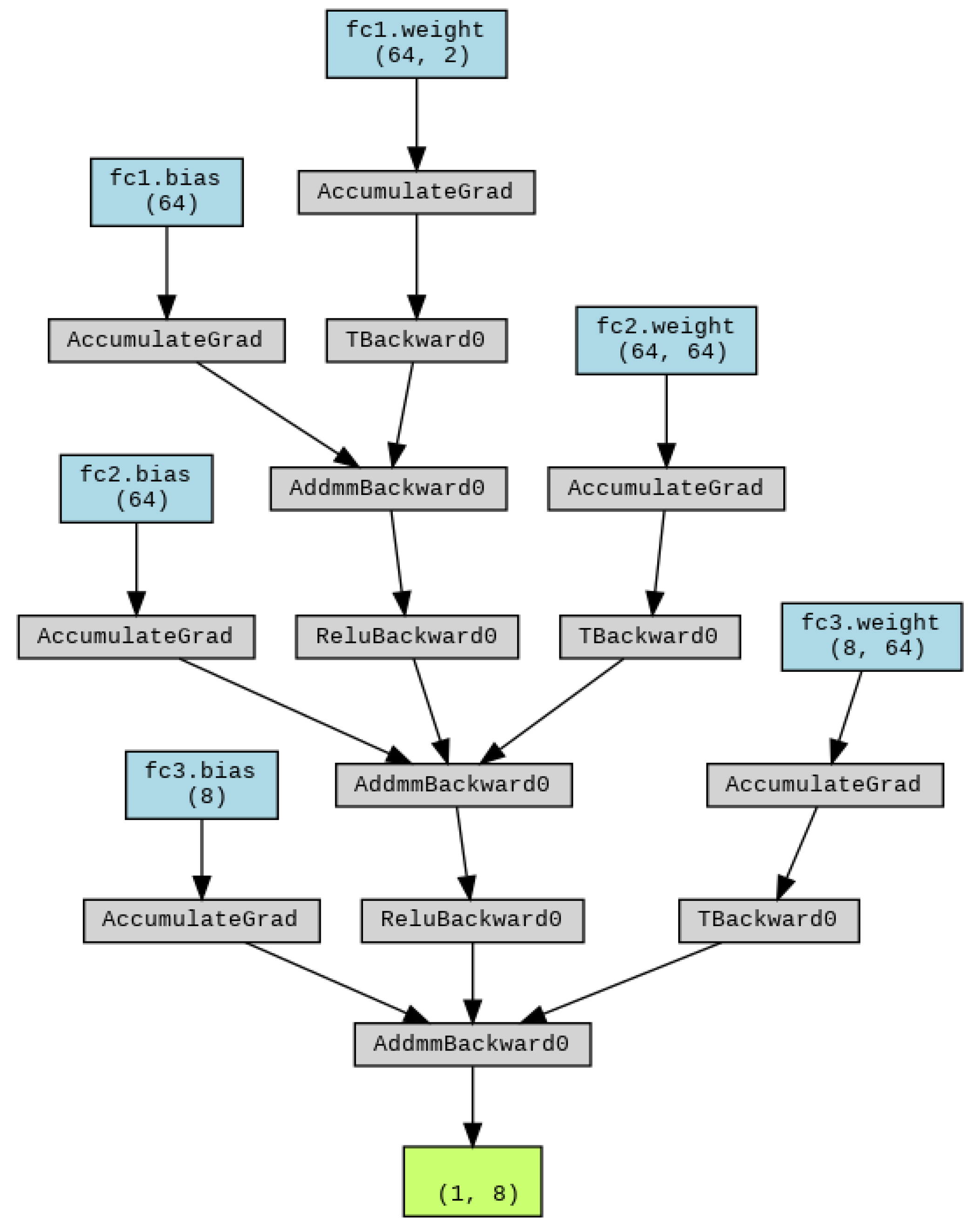
• Input layer: two fully connected neurons, one for the $x$ position and one for the $y$ position.
• Hidden layers: two fully connected layers with 64 neurons and the ReLU activation function.
• Output layer: a fully connected dense layer, which has 64 neurons as the input to the last hidden layer. It produces a vector $(1, 8)$ that corresponds to the Q values for each possible action in an environment.

Table 2 describes the hyperparameters selected for this study. Selecting a high discount rate allows the agent to pursue a greater reward in the long term. As the discount rate decreases, the agent will pursue short-term payoffs. A low learning rate translates into slow convergence, so a high number of episodes is necessary to guarantee convergence with a low learning rate. A high learning rate can result in network divergence.

Table 2. Hyperparameters of the Deep Q-Learning algorithm.

Parameter	Value
Episodes	1000
Learning rate, α	1 × 10−3
Random probability starts	1
Random probability end	1 × 10−2
Random probability decay	0.995
Target update frequency, θ	10
Discount rate, γ	0.99
Memory size	10,000

The algorithm was developed in Python programming with support from the open-source framework TensorFlow. The hardware settings are the same as those of the policy iteration algorithm.

2.3. Controller Design for Path Tracking

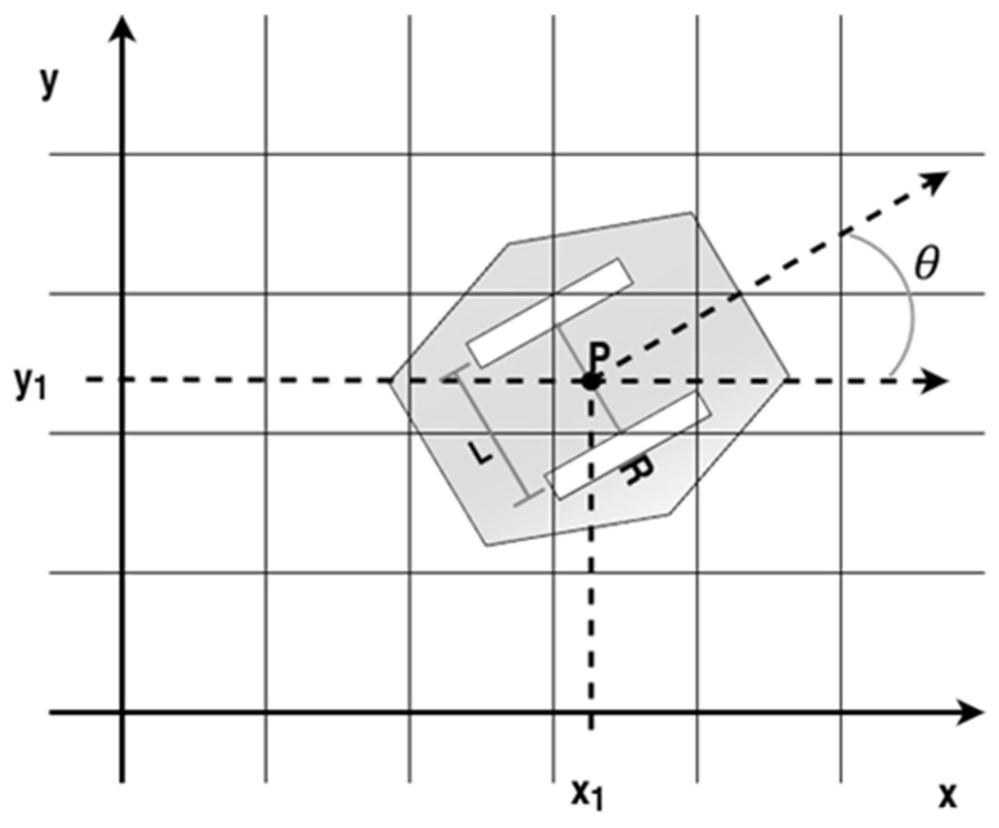
2.3.1. Kinematic Model of a Differential Drive Robot

The locomotion system, the environment in which it operates, and the number of wheels determine the type of movement of a system [30,31]. Differential drive is obtained by independently turning the two wheels, which are connected to the same axis but operate independently. There is often an additional support wheel to improve stability.

Figure 7 shows a differential drive robot on coordinates $x-y$; for kinematic analysis, the following is assumed:

Figure 7. Arbitrary top view of the platform with respect to the global reference frame.

• The robot is treated as a rigid body, as evidenced by its elements.
• Displacement is minimized in a perpendicular direction to the rolling.
• There is no translational displacement between the wheel and the floor.

The $x$ and $y$ velocities of the robot depend on the linear velocity, $v$, and are represented as follows:

$$\stackrel{·}{x}=v·\cos \theta$$

(14)

$$\stackrel{·}{y}=v·\sin \theta$$

(15)

For the angular velocity, $\stackrel{·}{\theta }$, we have the following expression:

$$\stackrel{·}{\theta }=\omega$$

(16)

The kinematic model of a differential drive robot is represented in Equation (17):

$$\left[\begin{array}{c}\stackrel{·}{x}\\ \stackrel{·}{y}\\ \stackrel{·}{\theta }\end{array}\right]=\left[\begin{array}{cc}\cos \theta & 0\\ \sin \theta & 0\\ 0& 1\end{array}\right]\left[\begin{array}{c}v\\ \omega \end{array}\right]$$

(17)

Considering the kinematic model, it is possible to differentiate equations that describe the movement of the robot, where $vr$ is the velocity of the right wheel and $vl$ is the velocity of the left wheel, both in $\mathrm{r}\mathrm{a}\mathrm{d}⁄\mathrm{s}$, $R$ represents the radius of the wheel, and $L$ represents the distance between wheels. The lineal velocity, $v$, and angular velocity, ω, are shown in Equations (18) and (19), respectively [32]:

$$v=R{\displaystyle \frac{\left(vr+vl\right)}{2}}$$

(18)

$$\omega =R{\displaystyle \frac{\left(vr+vl\right)}{L}}$$

(19)

2.3.2. Lyapunov-Based Controller Design

The Lyapunov-based controller design involves the selection of a suitable Lyapunov function, the analysis of its derivatives in order to guarantee its stability, and the design of a control law that uses this function to lead the system towards a desired behavior [33]. In a $\stackrel{·}{x}=f(x,u)$ system, a control Lyapunov function, $V$, is a positive-defined function for which the following is the case [34]:

$$\forall x\ne 0,\exists u \stackrel{·}{V}\left(x,u\right)={\displaystyle \frac{\partial V}{\partial x}}f\left(x,u\right)<0 \mathrm{and} \exists u \stackrel{·}{V}\left(0,u\right)=0$$

(20)

It assumes that for the whole value of $x$, there is a control variable that minimizes.

Assuming that there is a trajectory of movement, $r\left(t\right)$, the point of interest is based on its velocity, $\stackrel{·}{r}\left(t\right)$, and its conditions in the initial position as well as its orientation. It is possible to obtain the velocity of each point of the trajectory through a Jacobian matrix, $J\left(q\right(t\left)\right)$, under the assumption that $J\left(q\right(t\left)\right)$ is regular and therefore that the inverse exists. The vector of the joint velocities is calculated as follows [19,33]:

$$\stackrel{·}{q}\left(t\right)={J\left(q\right(t\left)\right)}^{-1}·r\left(t\right)$$

(21)

where $\stackrel{·}{q}\left(t\right)$ is the velocities conjoined through a given trajectory. The path error can be included in the inverse kinematics calculation. Equation (21) is rewritten as follows:

$$\stackrel{·}{q}\left[k\right]={J\left(q\left[k\right]\right)}^{-1}·{(r}_d\left[k\right]-r_e\left[k\right])$$

(22)

where $r_d$ is the desired state and $r_e$ is the actual state. To prove the stability of the closed-loop system, we propose the root mean square error as a Lyapunov function in its matrix form:

$$V(r_e)={\displaystyle \frac{r_e^T{·r}_e}{2}}$$

(23)

The function $V\left(r_e\right)$ is locally positive in $D$. That is, $V\left(0\right)=0$ and $V\left(r_e\right)>0$ in $D-\left\{0\right\}.$ for all $r_e$ in $D$. Its derivation can be represented as follows:

$$\stackrel{·}{V}\left(r_e\right)=r_e^T\stackrel{·}{{·r}_e}$$

(24)

$\stackrel{·}{V}\left(r_e\right)\le 0$ for all $r_e$ in $D$; therefore, it is asymptotically stable [35]. In order to assess stability, the expression of the derivative of the nominated function in the function of the velocity of the error is presented as

$$\stackrel{·}{r_e}=-K·r_e$$

(25)

where $K$ is a proposal positive-defined matrix. Substituting Equation (25) into (22), we obtain the control equation

$$\stackrel{·}{q}\left[k\right]={J\left(q\left[k\right]\right)}^{-1}·K·r_e\left[k\right]$$

(26)

Algorithm 3 is the controller algorithm to be applied.

Algorithm 3: Lyapunov-Based Controller
1:	Initialize
2:	$Samples,robot parameters,desired trajectory$.
3:	Controller Calculation
4:	Loop:
5:	$Error calculation$.
6:	Jacobian matrix J(q(t)).
7:	Control parameters.
8:	$Control law \stackrel{·}{q}\left[k\right]={J\left(q\left[k\right]\right)}^{-1}·K·r_e\left[k\right]$
9:	$Control actions$.
10:	End Loop
11:	Visualization

3. Results

This section is divided into two subsections.

The first subsection examines the variation in the distance and number of turns of the proposed RL and Deep Q-Learning algorithms in comparison to A*. The first A* algorithm considers four actions and the second eight actions.

The second subsection presents the results of the controller for the follow-up of trajectories based on the Lyapunov candidate function.

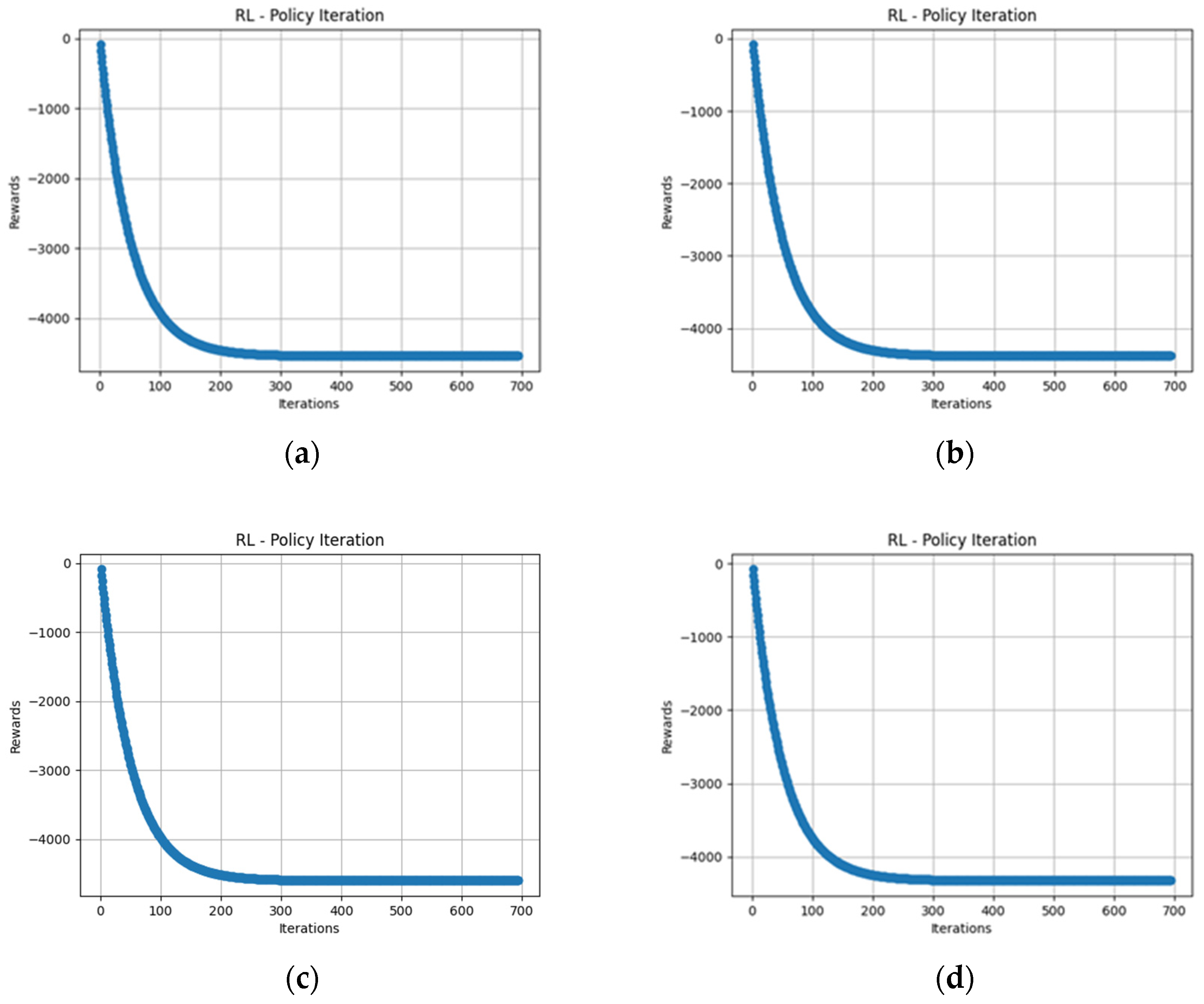
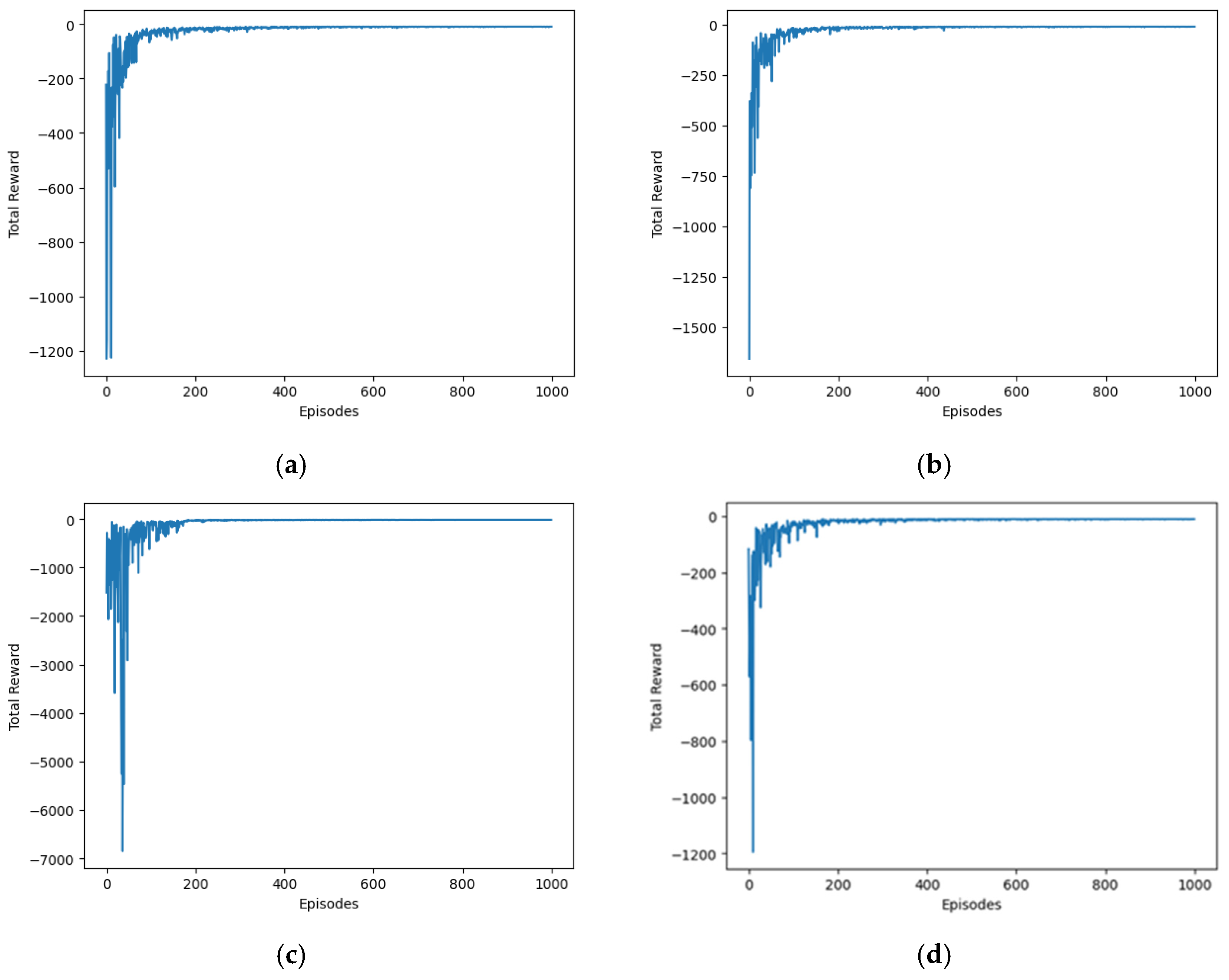
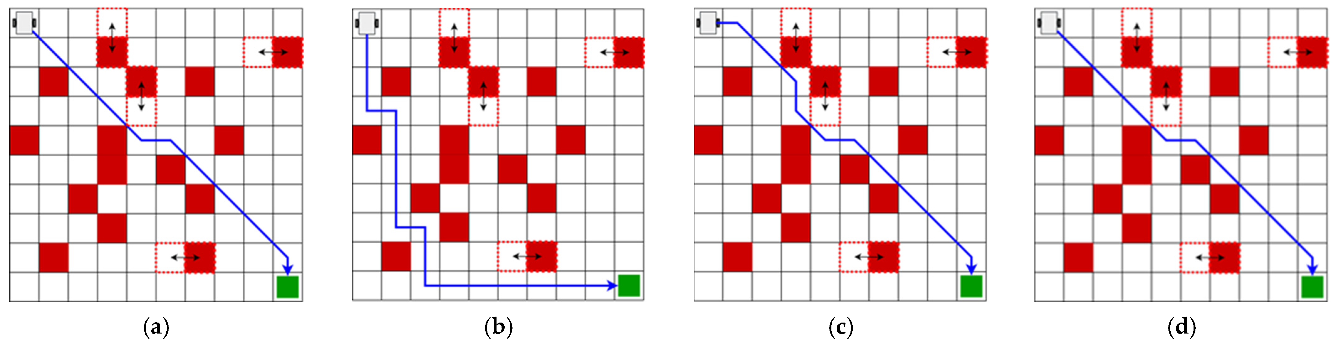
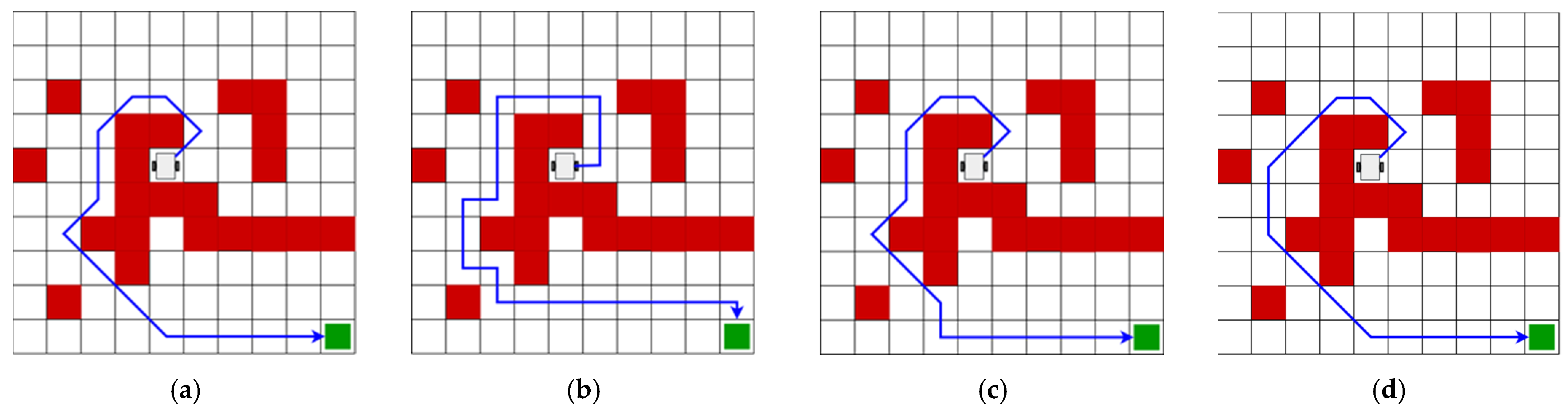
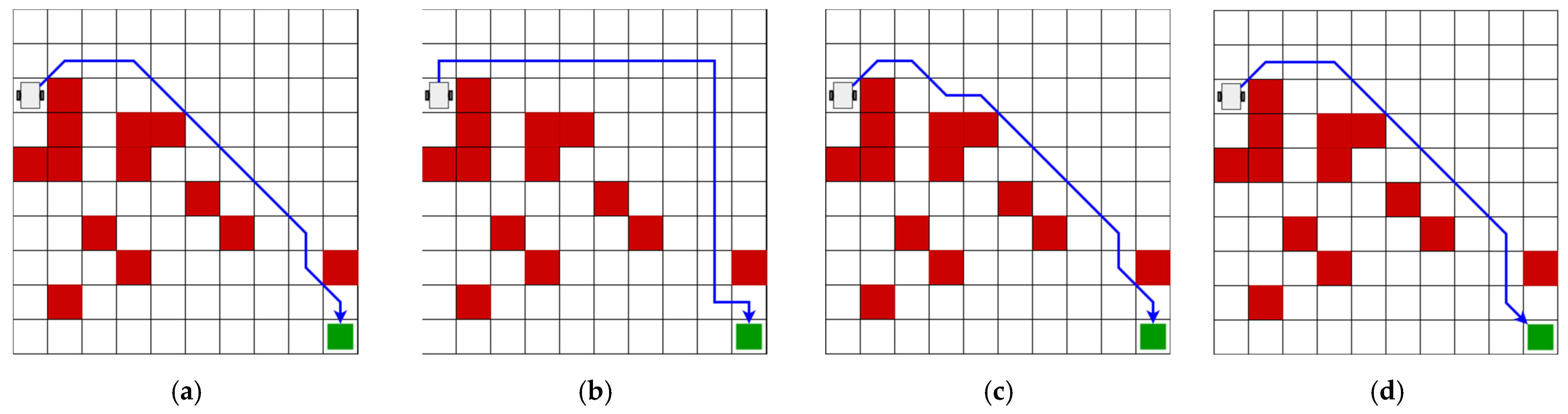
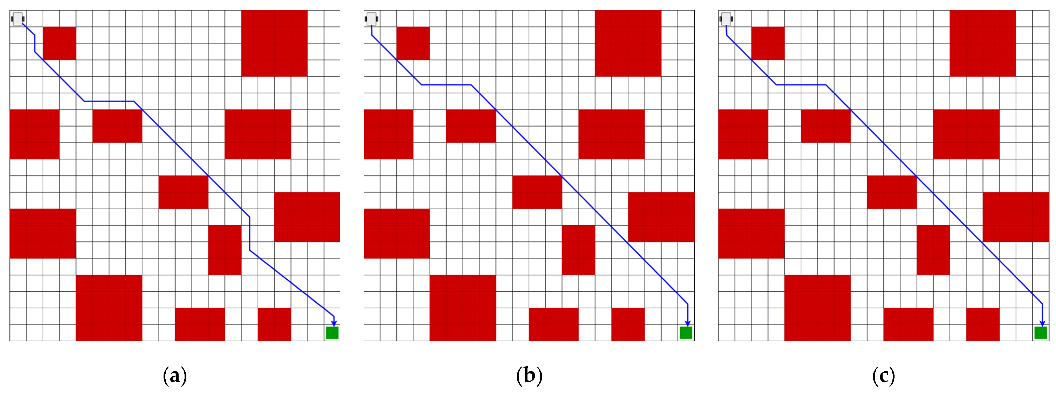
3.1. Evaluation of Trajectory-Planning Algorithms

Figure 8 shows the proposed maps for the evaluation of the algorithms RL and Deep Q-Learning. Four different maps are considered.

Figure 8. The structures of the maps used for the test: (a) Map 1, with static obstacles and a dynamic obstacle; (b) Map 2, with static and dynamic obstacles; (c) Map 3, with static obstacles; and (d) Map 4, with static obstacles.

The first map, proposed in Figure 8a, contemplates the initial position of the agent at the coordinate $(0, 0)$, corresponding to the upper-left corner. In this environment, a vertical, obstacle-free trajectory from the initial row to the final row of fixed obstacles is avoided. The only trajectory that has this characteristic is planned by horizontally moving a dynamic obstacle, which changes in each iteration. The objective is located in the lower-right corner, corresponding to position $(9, 9).$

The second proposed map, shown in Figure 8b, is a variant of the first map and aims to validate the agent behavior by adding random dynamic obstacles.

The third and fourth maps are shown in Figure 8c and Figure 8d, respectively. They contemplate static obstacles, but an initial coordinate different from the coordinate $(0, 0)$ is considered.

Figure 9a–d shows the graphs of the number of iterations with rewards from the RL algorithm for Maps 1, 2, 3, and 4, respectively. Map 1 shows a total reward of 4539, while Map 2 shows 4381, Map 3 shows 4323, and Map 4 shows 4596. All four graphs indicate a tendency to minimize accumulated rewards. The close values between the accumulated rewards of the maps are due to the fact that each map considers 10 × 10 cells, and the action sequences for each map have similar lengths. From iteration 300 onwards, convergence is evident in each map.

Figure 9. Rewards versus iterations of the RL algorithm. (a) Rewards versus iterations, Map 1; (b) rewards versus iterations, Map 2; (c) rewards versus iterations, Map 3; and (d) rewards versus iterations, Map 4.

Figure 10 shows the performance of the proposed Deep Q-Learning algorithm. The rewards versus episode plots for Maps 1, 2, 3, and 4 are seen in Figure 10a, Figure 10b, Figure 10c, and Figure 10d, respectively. The four graphs show a convergence from episode 200 onwards. The results show acceptable performance, since the agent receives minimum penalties along the trajectory. This can be proven with values close to zero from episode 200 onwards.

Figure 10. Reward versus episodes of the RL algorithm. (a) Rewards versus episodes, Map 1; (b) rewards versus episodes, Map 2; (c) rewards versus episodes, Map 3; and (d) rewards versus episodes, Map 4.

The characteristics to be compared with the four proposed algorithms include the distance traveled, the number of turns during the trajectory, and the training time. Table 3 provides a comparison based on the planted approach.

Table 3. Comparison of the performance of each algorithm on different maps.

Map	Algorithm	Distance (m)	No. Turns	Training Time (s)
	Reinforcement learning	13.89	3	112.40
1	Deep Q-Learning	13.89	3	526.45
	A* (4 actions)	22.00	10	0.011
	A* (8 actions)	13.89	4	0.015
	Reinforcement Learning	13.31	4	119.46
2	Deep Q-Learning	13.31	4	556.49
	A* (4 actions)	18.00	5	0.011
	A* (8 actions)	13.89	7	0.014
	Reinforcement learning	17.89	8	127.65
3	Deep Q-Learning	17.89	7	687.87
	A* (4 actions)	22.00	10	0.010
	A* (8 actions)	18.48	9	0.014
	Reinforcement learning	13.89	6	98.06
4	Deep Q-Learning	13.89	4	447.16
	A* (4 actions)	18.00	4	0.009
	A* (8 actions)	13.89	8	0.013

The graphical representation of the optimal trajectory of the four algorithms proposed in Maps 1, 2, 3, and 4 is presented in Figure 11, Figure 12, Figure 13, and Figure 14, respectively. The response of each algorithm is shown separately.

Figure 11. The optimal trajectory of Map 1 according to the proposed algorithms. (a) Optimal trajectory of the RL algorithm of Map 1; (b) optimal trajectory of the A*-4 algorithm of Map 1; (c) optimal trajectory of the A*-8 algorithm of Map 1; and (d) optimal trajectory of the Deep Q-Learning algorithm of Map 1.

Figure 12. The optimal trajectory of Map 2 according to the proposed algorithms. (a) Optimal trajectory of the RL algorithm of Map 2; (b) optimal trajectory of the A*-4 algorithm of Map 2; (c) optimal trajectory of the A*-8 algorithm of Map 2; and (d) optimal trajectory of the Deep Q-Learning algorithm of Map 2.

Figure 13. The optimal trajectory of Map 3 according to the proposed algorithms. (a) Optimal trajectory of the RL algorithm of Map 3; (b) optimal trajectory of the A*-4 algorithm of Map 3; (c) optimal trajectory of the A*-8 algorithm of Map 3; and (d) optimal trajectory of the Deep Q-Learning algorithm of Map 3.

Figure 14. The optimal trajectory of Map 4 according to the proposed algorithms. (a) Optimal trajectory of the RL algorithm of Map 4; (b) optimal trajectory of the A*-4 algorithm of Map 4; (c) optimal trajectory of the A*-8 algorithm of Map 4; and (d) optimal trajectory of the Deep Q-Learning algorithm of Map 4.

To prove the advantages of the proposed model of trajectory planning, we compared it to the ID3QN [36] and DQN [37] models under the same conditions. The DQN [37] model shows a higher performance compared to the method in [36] in terms of the number of turns and a lower performance in the length of the trajectory. The ID3QN method adopts a structure of three fully connected hidden layers with 256 neurons and applies the ReLU activation function.

Figure 15 shows the trajectory of each algorithm in a map of 20 × 20 cells. The length of the trajectory in all maps is 28.627. The number of turns for the ID3QN and DQN algorithms and the proposed DQL method is 7, 4, and 4, respectively.

Figure 15. The optimal trajectory of algorithms in a map of 20 × 20 cells. (a) Optimal trajectory of the ID3QN algorithm; (b) optimal trajectory of the DQN algorithm; and (c) optimal trajectory of the proposed DQL algorithm.

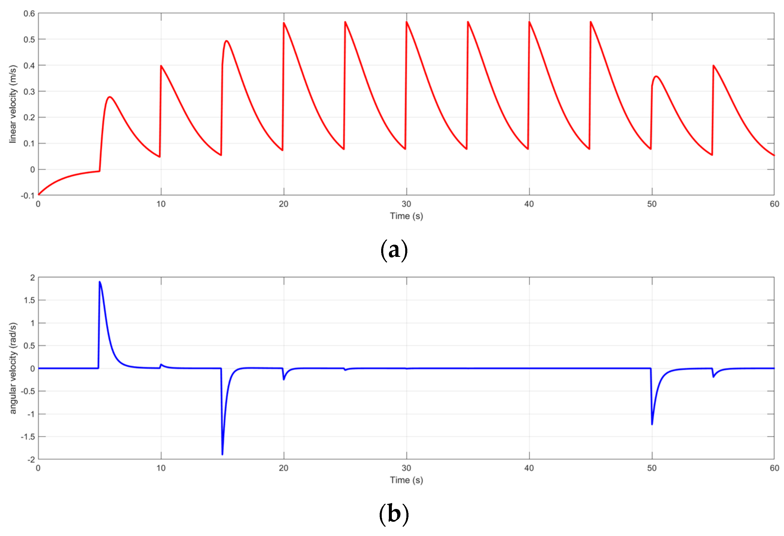
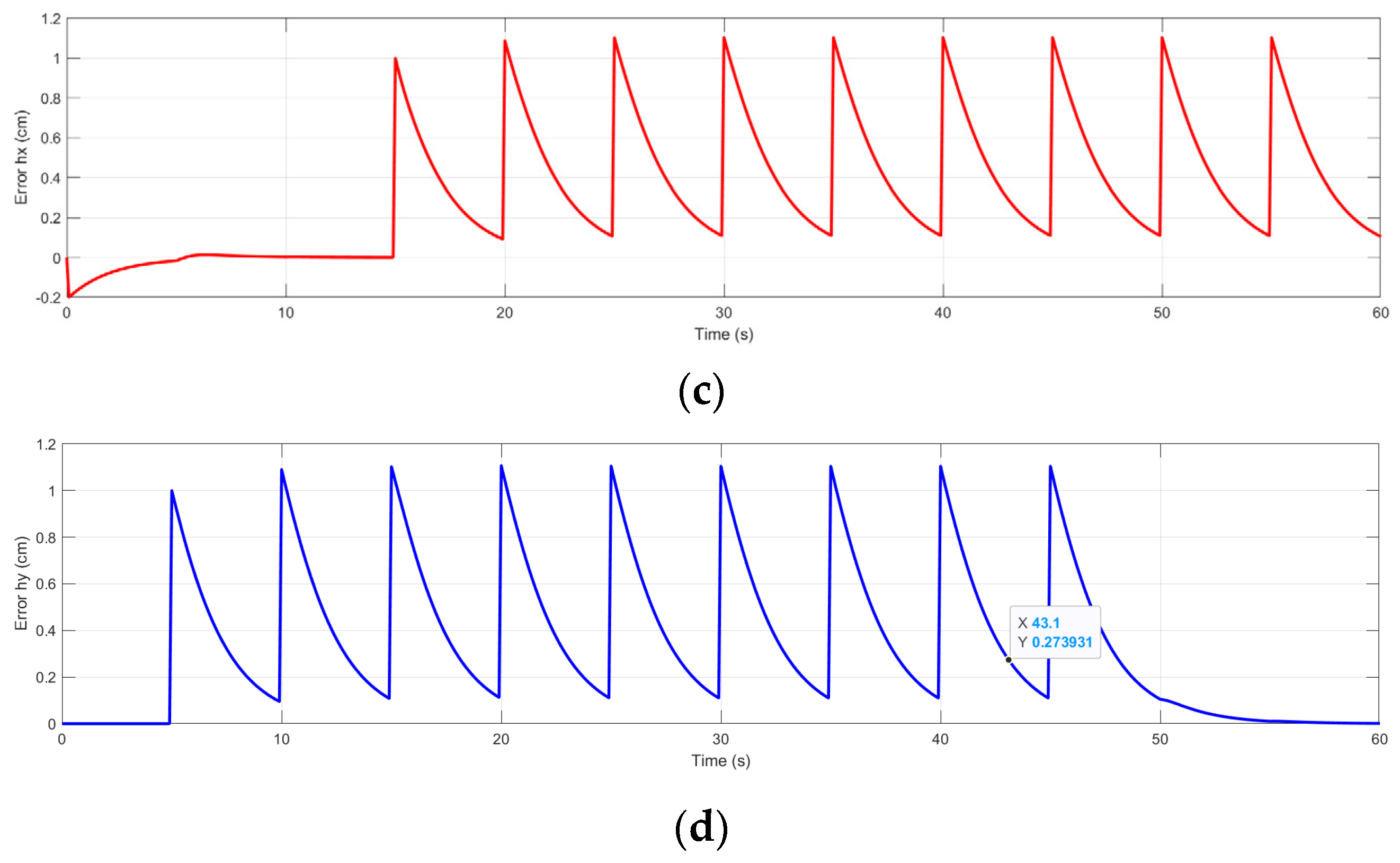
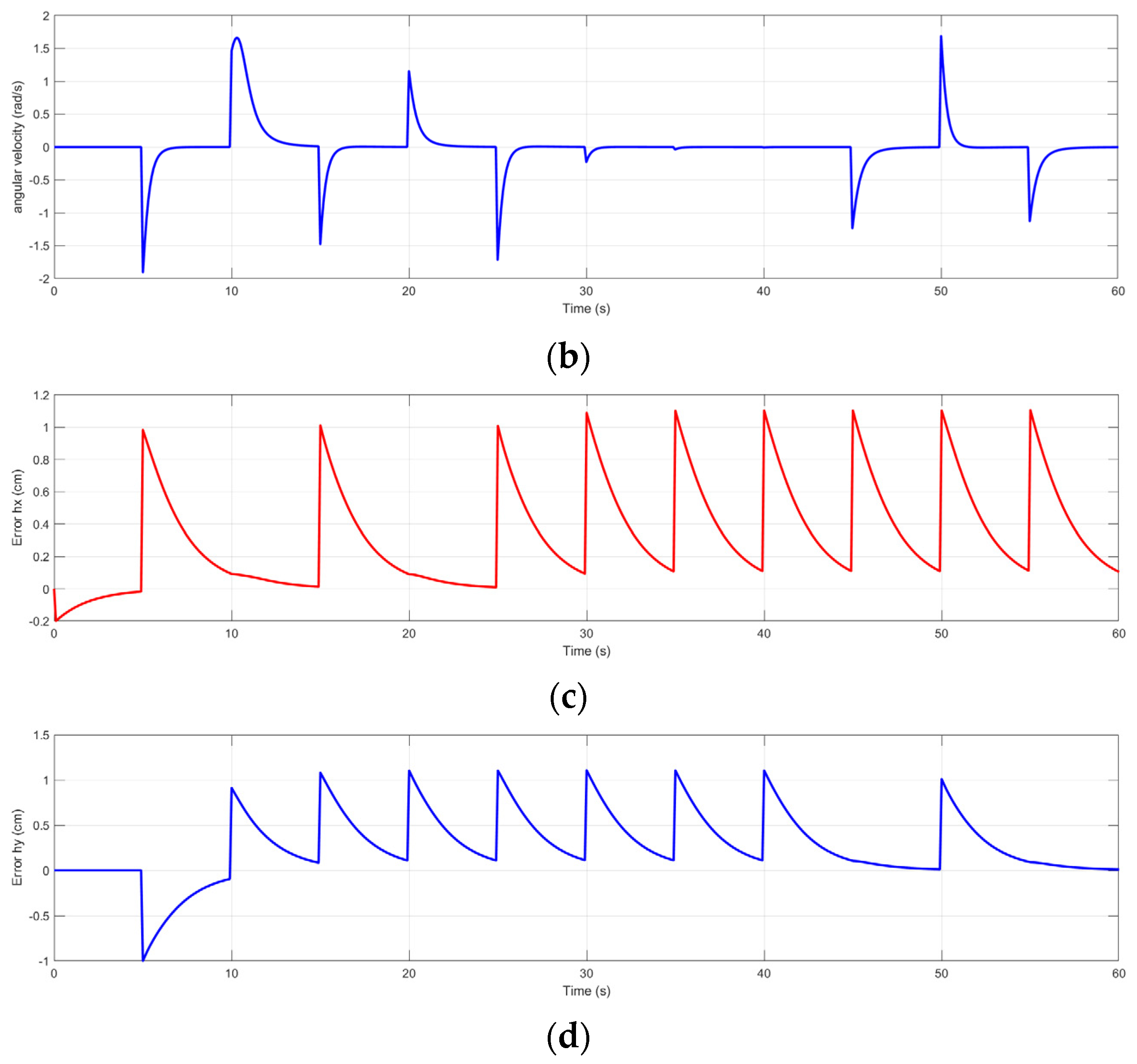
3.2. Results of the Trajectory-Tracking Controller Design

In this second part, the response of the controller for trajectory tracking on the different maps is presented. The controller’s response was evaluated using the optimal trajectory of the DQL algorithm, which showed the best performance compared to the other proposed algorithms.

The estimated desired trajectory for the four maps is presented in Figure 16. The configuration used for the robot to evaluate the performance control is as follows: $L=0.5 \mathrm{m}$ and $r=0.15 \mathrm{m}$. The $K$ parameter proposed for the controller is 0.1.

Figure 16. The desired trajectory versus the estimated trajectory of the Deep Q Learning algorithm. (a) The desired trajectory versus the estimated trajectory of Map 1; (b) the desired trajectory versus the estimated trajectory of Map 2; (c) the desired trajectory versus the estimated trajectory of Map 3; (d) the desired trajectory versus the estimated trajectory of Map 4.

Figure 17, Figure 18, Figure 19 and Figure 20 show linear velocity and angular velocity, as well as errors in $x$ and $y$ for Maps 1, 2, 3, and 4.

Figure 17. The controller’s response for Deep Q-Learning algorithm trajectory for Map 1. (a) Linear velocity of robot in trajectory of Map 1; (b) angular velocity of robot in trajectory of Map 1; (c) error $x$ of robot in trajectory of Map 1; and (d) error $y$ of robot in trajectory of Map 1.

Figure 18. The controller’s response for the trajectory of the Deep Q-Learning algorithm for Map 2. (a) The linear velocity of the robot in the trajectory of Map 2; (b) the angular velocity of the robot in the trajectory of Map 2; (c) the error $x$ of the robot in the trajectory of Map 2; and (d) the error $y$ of the robot in the trajectory of Map 2.

Figure 19. The controller’s response for the trajectory of the Deep Q-Learning algorithm for Map 3. (a) The linear velocity of the robot in the trajectory of Map 3; (b) the angular velocity of the robot in the trajectory of Map 3; (c) the error $x$ of the robot in the trajectory of Map 3; and (d) the error $y$ of the robot in the trajectory of Map 3.

Figure 20. The controller’s response for the trajectory of the Deep Q-Learning algorithm for Map 4. (a) The linear velocity of the robot in the trajectory of Map 4; (b) the angular velocity of the robot in the trajectory of Map 4; (c) the error $x$ of the robot in the trajectory of Map 4; and (d) the error $y$ of the robot in the trajectory of Map 4.

4. Discussion

This section explores variations in the proposed algorithms within the four maps and the behavior of the trajectory-tracking controller.

The results demonstrate acceptable performance for both the basic RL and Deep Q-Learning algorithms. Both algorithms reduced the distance compared to the A* algorithm, which only had four probable actions. The A* algorithm achieved the same distance as the basic RL algorithm and the Deep Q-Learning algorithm, with eight possible actions, shown in Maps 1 and 4. The A* algorithm indicated a higher number of turns in all of the evaluated maps. Technique A* depended on knowledge of the environment, which limited its application in dynamic environments.

The RL algorithm and the Deep Q-Learning algorithm reduced the number of turns in all maps, resulting in a balance between trajectory distance and the number of turns.

The difference between the RL algorithm and the Deep Q-Learning algorithm lay in the number of turns along the trajectory. The Deep Q-Learning algorithm reduced the number of turns in Maps 3 and 4. This allowed the robot to maintain a constant velocity along most of its trajectory.

The behavior of the RL algorithm and the Deep Q-Learning algorithm allowed us to verify that the proposed reward function motivated the agent to take shorter paths with fewer turns in comparison to the A* technique. The reward function employed in the basic RL algorithm and the Deep Q-Learning algorithm accomplished the objective of incentivizing an agent to take diagonal paths with the minimum number of turns. This approach allowed the robot to save energy by maintaining a constant velocity for an extended period of time.

The RL and Deep Q-Learning algorithms found an optimal path without prior knowledge of the locations of the obstacles and their dynamics without updating the probability of displacement. The proposed dynamic environments did not represent a problem for any of the algorithms in determining the optimal path since the dynamic obstacles had minimal motion in the environment.

The reward function employed in the basic RL algorithm and the Deep Q-Learning algorithm accomplished the objective of incentivizing the agent to take diagonal trajectories with the minimum number of turns. This approach allowed the robot to save energy by maintaining a constant velocity for as long as possible.

The proposed method was evaluated using two RL-based algorithms. The result was the same performance as the ID3QN and DQN algorithms in the length of the trajectory. Regarding the number of turns, the ID3QN algorithm showed a higher performance compared to the DQN algorithm and the proposed method. Additionally, the proposed algorithm showed a reduction in the number of neurons from 256 to 64 and a reduction in the number of hidden layers from three to two compared to the ID3QN method. This represents a reduction in computational resources.

Trajectory control based on the Lyapunov candidate was proposed, which corresponds to a mean square error that meets the two stability conditions.

The error between the desired trajectory and the estimated trajectory was less than $1.2 \mathrm{c}\mathrm{m}$ in axis $x$ and $y$.

5. Conclusions

As a result, the proposed reward function met the objective of motivating an agent to find the shortest route with fewer turns in comparison to the classic A* technique. The use of the reward function allowed for a reduction in turns in all cases of up to 50%, and showed a distance reduction of 36% against algorithm A* with four probable actions and 3.2% for algorithm A* with eight probable actions.

The root mean square error was evaluated as a potential candidate function for the Lyapunov-based controller. The root mean square complied with the Lyapunov stability criteria. Simulations showed the efficiency of the proposed scheme, which provided the robot with smooth and accurate motions. The angular velocity showed minimal variation, resulting in a smooth trajectory from the initial point to the target point.

6. Future Work

• Conduct a comparison of the controller’s performance in real environments against the results obtained analytically.
• Integrate deep learning algorithms to provide visual feedback for the robot and determine the locations of dynamic obstacles as well as the behavior in these environments, with the objective of updating the values of compensation dynamically.
• Study and propose techniques for interpolation to smooth trajectories between cells, which, combined with visual feedback, can generate new routes with constant velocities.
• Assess other algorithms based on reinforcement learning and establish new functions for rewards and the initiation of states.
• Evaluate the learning by reinforcement algorithms on maps with a larger number of cells to validate convergence.

References

- Mohanty, P.K.; Singh, A.K.; Kumar, A.; Mahto, M.K.; Kundu, S. Path Planning Techniques for Mobile Robots: A Review. In Lecture Notes in Networks and Systems, Proceedings of the 13th International Conference on Soft Computing and Pattern Recognition (SoCPaR 2021); Springer: Cham, Switzerland, 2022; Volume 417. [Google Scholar] [CrossRef]
- Cheng, C.X.; Sha, Q.X.; He, B.; Li, G.L. Path planning and obstacle avoidance for AUV: A review. Ocean Eng. 2021, 235, 109355. [Google Scholar] [CrossRef]
- Loganathan, A.; Ahmad, N.S. A systematic review on recent advances in autonomous mobile robot navigation. Eng. Sci. Technol. 2023, 40, 101343. [Google Scholar] [CrossRef]
- Wu, M.; Yeong, C.F.; Su, E.L.M.; Holderbaum, W.; Yang, C. A review on energy efficiency in autonomous mobile robots. Robot. Intell. Autom. 2023, 43, 648–668. [Google Scholar] [CrossRef]
- Liu, L.X.; Wang, X.; Yang, X.; Liu, H.J.; Li, J.P.; Wang, P.F. Path planning techniques for mobile robots: Review and prospect. Expert Syst. Appl. 2023, 227, 120254. [Google Scholar] [CrossRef]
- Salama, O.A.A.; Eltaib, M.E.H.; Mohamed, H.A.; Salah, O. RCD: Radial Cell Decomposition Algorithm for Mobile Robot Path Planning. IEEE Access 2021, 9, 149982–149992. [Google Scholar] [CrossRef]
- Chen, G.; Luo, N.; Liu, D.; Zhao, Z.; Liang, C. Path planning for manipulators based on an improved probabilistic roadmap method. Robot. Comput. Integr. Manuf. 2021, 72, 102196. [Google Scholar] [CrossRef]
- Souza, R.M.J.A.; Lima, G.V.; Morais, A.S.; Oliveira-Lopes, L.C.; Ramos, D.C.; Tofoli, F.L. Modified Artificial Potential Field for the Path Planning of Aircraft Swarms in Three-Dimensional Environments. Sensors 2022, 22, 1558. [Google Scholar] [CrossRef]
- Lindqvist, B.; Agha-Mohammadi, A.A.; Nikolakopoulos, G. Exploration-RRT: A multi-objective Path Planning and Exploration Framework for Unknown and Unstructured Environments. arXiv 2021, arXiv:2104.03724. [Google Scholar] [CrossRef]
- Low, E.S.; Ong, P.; Low, C.Y. A modified Q-learning path planning approach using distortion concept and optimization in dynamic environment for autonomous mobile robot. Comput. Ind. Eng. 2023, 181, 109338. [Google Scholar] [CrossRef]
- Zaharuddeen, H.; Muhammed Bashir, M.A.; Abubakar, U.; Glory Okpowodu, U. Path Planning Algorithms for Mobile Robots: A Survey. In Motion Planning for Dynamic Agents; Zain Anwar, A., Amber, I., Eds.; IntechOpen: Rijeka, Croatia, 2023; Chapter 5. [Google Scholar]
- Gad, A.G. Particle Swarm Optimization Algorithm and Its Applications: A Systematic Review (Apr, 10.1007/s11831-021-09694-4, 2022). Arch. Comput. Method E 2023, 30, 3471. [Google Scholar] [CrossRef]
- Arulkumaran, K.; Deisenroth, M.P.; Brundage, M.; Bharath, A.A. Deep Reinforcement Learning: A Brief Survey. IEEE Signal Process. Mag. 2017, 34, 26–38. [Google Scholar] [CrossRef]
- Li, S.E. Reinforcement Learning for Sequential Decision and Optimal Control; Springer: Singapore, 2023. [Google Scholar]
- Sutton, R.S.; Barto, A.G. Reinforcement Learning: An Introduction, 2nd ed.; A Bradford Book: London, UK, 2018. [Google Scholar]
- Lan, W.; Jin, X.; Chang, X.; Wang, T.; Zhou, H.; Tian, W.; Zhou, L. Path planning for underwater gliders in time-varying ocean current using deep reinforcement learning. Ocean Eng. 2022, 262, 112226. [Google Scholar] [CrossRef]
- Li, Z.; Wu, L.; Xu, Y.; Moazeni, S.; Tang, Z. Multi-Stage Real-Time Operation of a Multi-Energy Microgrid with Electrical and Thermal Energy Storage Assets: A Data-Driven MPC-ADP Approach. IEEE Trans. Smart Grid 2022, 13, 213–226. [Google Scholar] [CrossRef]
- Gao, H.; Jiang, S.; Li, Z.; Wang, R.; Liu, Y.; Liu, J. A Two-stage Multi-agent Deep Reinforcement Learning Method for Urban Distribution Network Reconfiguration Considering Switch Contribution. IEEE Trans. Power Syst. 2024, 1–12. [Google Scholar] [CrossRef]
- Xu, C.; Zhao, W.; Chen, Q.; Wang, C. An actor-critic based learning method for decision-making and planning of autonomous vehicles. Sci. China Technol. Sci. 2021, 64, 984–994. [Google Scholar] [CrossRef]
- Zhou, S.; Liu, X.; Xu, Y.; Guo, J. A Deep Q-network (DQN) Based Path Planning Method for Mobile Robots. In Proceedings of the 2018 IEEE International Conference on Information and Automation (ICIA), Wuyishan, China, 11–13 August 2018; pp. 366–371. [Google Scholar]
- Low, E.S.; Ong, P.; Low, C.Y. An empirical evaluation of Q-learning in autonomous mobile robots in static and dynamic environments using simulation. Decis. Anal. J. 2023, 8, 100314. [Google Scholar] [CrossRef]
- Low, E.S.; Ong, P.; Low, C.Y.; Omar, R. Modified Q-learning with distance metric and virtual target on path planning of mobile robot. Expert Syst. Appl. 2022, 199, 117191. [Google Scholar] [CrossRef]
- Maoudj, A.; Hentout, A. Optimal path planning approach based on Q-learning algorithm for mobile robots. Appl. Soft Comput. 2020, 97, 106796. [Google Scholar] [CrossRef]
- Low, E.S.; Ong, P.; Cheah, K.C. Solving the optimal path planning of a mobile robot using improved Q-learning. Robot. Auton. Syst. 2019, 115, 143–161. [Google Scholar] [CrossRef]
- Chen, C.; Chen, X.-Q.; Ma, F.; Zeng, X.-J.; Wang, J. A knowledge-free path planning approach for smart ships based on reinforcement learning. Ocean Eng. 2019, 189, 106299. [Google Scholar] [CrossRef]
- Huo, F.; Zhu, S.; Dong, H.; Ren, W. A new approach to smooth path planning of Ackerman mobile robot based on improved ACO algorithm and B-spline curve. Robot. Auton. Syst. 2024, 175, 104655. [Google Scholar] [CrossRef]
- Elhoseny, M.; Tharwat, A.; Hassanien, A.E. Bezier Curve Based Path Planning in a Dynamic Field using Modified Genetic Algorithm. J. Comput. Sci. 2018, 25, 339–350. [Google Scholar] [CrossRef]
- Bellman, R. A Markovian Decision Process. J. Math. Mech. 1957, 6, 679–684. [Google Scholar] [CrossRef]
- Pieters, M.; Wiering, M.A. Q-learning with experience replay in a dynamic environment. In Proceedings of the 2016 IEEE Symposium Series on Computational Intelligence (SSCI), Athens, Greece, 6–9 December 2016; pp. 1–8. [Google Scholar]
- Xie, M. Fundamentals of Robotics: Linking Perception to Action; World Scientific Publishing Company: Singapore, 2003. [Google Scholar]
- de Wit, C.A.C.; Siciliano, B.; Bastin, G. Theory of Robot Control; Springer: London, UK, 1996. [Google Scholar]
- Rapalski, A.; Dudzik, S. Energy Consumption Analysis of the Selected Navigation Algorithms for Wheeled Mobile Robots. Energies 2023, 16, 1532. [Google Scholar] [CrossRef]
- Lewis, F.L.; Dawson, D.M.; Abdallah, C.T. Robot Manipulator Control: Theory and Practice, Revised and Expanded; Taylor & Francis Group: Abingdon, UK, 2003. [Google Scholar]
- Tedrake, R. Underactuated Robotics. Algorithms for Walking, Running, Swimming, Flying, and Manipulation (Course Notes for MIT 6.832). 2023. Available online: http://underactuated.mit.edu (accessed on 8 May 2023).
- Kubo, R.; Fujii, Y.; Nakamura, H. Control Lyapunov Function Design for Trajectory Tracking Problems of Wheeled Mobile Robot. IFAC-PapersOnLine 2020, 53, 6177–6182. [Google Scholar] [CrossRef]
- Wu, Z.; Yin, Y.; Liu, J.; Zhang, D.; Chen, J.; Jiang, W. A Novel Path Planning Approach for Mobile Robot in Radioactive Environment Based on Improved Deep Q Network Algorithm. Symmetry 2023, 15, 2048. [Google Scholar] [CrossRef]
- Wang, W.; Wu, Z.; Luo, H.; Zhang, B. Path Planning Method of Mobile Robot Using Improved Deep Reinforcement Learning. J. Electr. Comput. Eng. 2022, 2022, 5433988. [Google Scholar] [CrossRef]
Disclaimer/Publisher’s Note: The statements, opinions and data contained in all publications are solely those of the individual author(s) and contributor(s) and not of MDPI and/or the editor(s). MDPI and/or the editor(s) disclaim responsibility for any injury to people or property resulting from any ideas, methods, instructions or products referred to in the content. |
© 2024 by the authors. Licensee MDPI, Basel, Switzerland. This article is an open access article distributed under the terms and conditions of the Creative Commons Attribution (CC BY) license (https://creativecommons.org/licenses/by/4.0/).