Multi-Objective Five-Element Cycle Optimization Algorithm Based on Multi-Strategy Fusion for the Bi-Objective Traveling Thief Problem

Abstract

In this paper, we propose a Multi-objective Five-element Cycle Optimization algorithm based on Multi-strategy fusion (MOFECO-MS) to address the Bi-objective Traveling Thief Problem (BITTP), an extension of the Traveling Thief Problem that incorporates two conflicting objectives. The novelty of our approach lies in a unique individual selection strategy coupled with an innovative element update mechanism rooted in the Five-element Cycle Model. To balance global exploration and local exploitation, the algorithm categorizes the population into distinct groups and applies crossover operations both within and between these groups, while also employing a mutation operator for local searches on the best individuals. This coordinated approach optimizes parameter settings and enhances the search capabilities of the algorithm. Extensive experiments were conducted on nine BITTP instances, comparing MOFECO-MS against eight state-of-the-art multi-objective optimization algorithms. The results show that MOFECO-MS excels in both Hypervolume (HV) and Spread (SP) indicators, while also maintaining a high level of Pure Diversity (PD). Overall, MOFECO-MS outperformed the other algorithms in most instances, demonstrating its superiority and robustness in solving complex multi-objective optimization problems.

1. Introduction

Real-world optimization problems are inherently complex, often comprising multiple interdependent sub-problems. Traditionally, researchers address these challenges by decomposing such complex problems into independent sub-problems, solving them separately without considering their interactions. However, this approach overlooks the interdependencies among these sub-problems, leading to sub-optimal solutions that do not necessarily translate to optimal solutions for the entire problem [1].

To address this issue and better understand real-world complexities, the Traveling Thief Problem (TTP) was introduced as a benchmark problem [2]. TTP is a combinatorial optimization problem that integrates the Traveling Salesman Problem (TSP) and the Knapsack Problem (KP). The unique aspect of TTP lies in its ability to simulate the interdependencies between these two sub-problems, capturing the essence of real-world optimization scenarios where decisions made in one aspect of the problem influence outcomes in another. By modeling such interactions, TTP provides a more holistic approach to solving complex problems, making it a significant tool for researchers aiming to develop optimization algorithms that are more applicable to real-world situations.

In the context of TTP, two variants are commonly studied: the single-objective TTP and the bi-objective TTP (BITTP), which is the focus of this paper. The BITTP not only seeks to optimize the route and item selection to minimize travel time and maximize profit but also offers a framework for studying trade-offs between conflicting objectives, which is crucial for real-world decision-making processes.

Numerous scholars have explored diverse methodologies to tackle the single-objective TTP, leveraging a spectrum of approaches ranging from heuristic algorithms [3,4,5,6] to swarm intelligence optimization techniques [7,8,9,10].

In recent years, the Bi-Objective Traveling Thief Problem (TTP) has garnered significant attention, with various approaches being developed to address its unique challenges. The complexity of TTP arises from the interdependence between the Traveling Salesman Problem and the Knapsack Problem, making traditional single-objective methods insufficient. To tackle these challenges, researchers have proposed a range of multi-objective evolutionary algorithms, hybrid approaches combining dynamic programming, and specialized metaheuristics. These methods aim to optimize both the journey time and the total value of collected items while addressing the interrelated nature of the sub-problems.

For instance, several studies have focused on multi-objective evolutionary algorithms, such as NSGA-II and its variants, which demonstrate robust performance across various TTP instances [11]. Others have integrated dynamic programming within evolutionary frameworks, showing significant improvements in solution quality, particularly for large instances [12]. Additionally, adaptive and specialized algorithms tailored to the unique facets of TTP instances have been proposed [13], further enhancing the effectiveness of these methods. Metaheuristic approaches like Variable Neighbourhood Search [14] and weighted-sum methods [15] have also been explored, offering competitive results compared to traditional optimization techniques. Moreover, the application of Ant Colony Optimization (ACO) [16] and the Imperialist Competitive Algorithm (ICA) has shown promise in improving best-known solutions across different TTP instances [17].

The following Table 1 summarizes these recent advancements in solving the Bi-Objective TTP, categorizing the studies based on their research focus, methods, and key contributions.

Table 1. Summary of Recent Studies on BITTP.

Study	Research Focus	Method	Key Contributions
Multi-Objective Evolutionary Algorithms  [11,12,13,18]	Solving Bi-Objective TTP using evolutionary algorithms	Establishes new benchmarks, demonstrates robust performance, and improves Pareto set approximations	Establishes new benchmarks, demonstrates robust performance, and improves Pareto set approximations
Dynamic Programming and Hybrid Approaches [12,16,19]	Integrating dynamic programming within evolutionary algorithms for TTP	Combines exact and approximate algorithms, leveraging DP for packing problems	Outperforms state-of-the-art results and enhances solution quality in large instances
Adaptive and Specialized Algorithms [11,13,20]	Dynamic multi-objective optimization of TTP	Combination of dynamic programming and evolutionary algorithms	Improves algorithm performance, particularly in specialized and adaptive contexts
Metaheuristic and Weighted-Sum Methods [14,15]	Utilizing metaheuristic approaches like VNS and weighted-sum methods	Includes randomized heuristics and Variable Neighbourhood Search	Provides competitive performance, improves best-known solutions in competitions
Ant Colony Optimization and ICA References [16,17,21]	Optimizing TTP with Ant Colony Optimization and Imperialist Competitive Algorithm	Combines MOEA/D with ACO and applies ICA to small instances	Achieves competitive results, improves multiple best-known solutions across instances

This paper introduces a novel heuristic multi-objective optimization algorithm for solving BITTP, leveraging the Five-element Cycle Optimization algorithm (FECO). FECO, grounded in the Five-element Cycle Model (FECM), has effectively addressed combinatorial optimization problems [22]. Building upon this framework, we devise a fresh individual evaluation criterion and integrate it with FECO’s distinctive optimization mechanism to formulate an innovative individual update strategy. This strategy aims to harmonize global exploration and local exploitation, enhancing search capabilities and facilitating more effective solutions to BITTP.

The remaining sections of the paper are organized as follows: Section 2 provides a comprehensive explanation of BITTP and FECO. The methodology for solving BITTP using the proposed algorithm is delineated in Section 3. Section 4 introduces the experimental conditions, including the experimental operating environment, benchmark problems, and algorithm performance metrics. Section 5 details the algorithm’s parameter settings, experimental results, and analysis. Finally, Section 6 offers concluding remarks and outlines avenues for future research.

2. Preliminaries

2.1. Bi-Objective Traveling Thief Problem

The TTP is a novel combinatorial optimization challenge that amalgamates two classical problems, the TSP and the KP. The BITTP, as adopted in this paper following the definition from [23], is a variant of TTP with dual objective functions. Specifically, it entails a scenario where a traveling thief traverses n cities while selectively acquiring items from a pool of $n^{\prime }$ items and placing them in their knapsack, ultimately returning to the departure city. Notably, the departure city does not contain any items, while other cities may contain one or more items. The objective is to devise an optimal route plan and item acquisition strategy to minimize the thief’s travel time while maximizing the total profit from the items. It is crucial to note the interdependence between the two objectives, as the selection of heavier items may impede the thief’s speed, thereby elongating travel time. The formulation of objective functions and constraints for BITTP is outlined below.

The route plan in the BITTP is represented by the vector $\mathit{\pi }=[{\pi }_1,{\pi }_2,\cdots ,{\pi }_i,\cdots ,{\pi }_n,{\pi }_1]$, where ${\pi }_i$ is a permutation vector denoting the sequence of cities visited by the thief. Here, ${\pi }_i$ represents the ith city visited by the thief, with i ranging from 1 to n.

The item plan represented as $\mathbf{z}$ is a vector denoted by $\mathbf{z}=[z_1,z_2,\cdots ,z_j,\cdots ,z_{n^{\prime }}]$, where $z_j$ corresponds to the jth item. Each element $z_j$ in $\mathbf{z}$ is a binary value: $z_j=1$ signifies that the jth item is selected, while $z_j=0$ indicates its exclusion. The index j ranges from 1 to $n^{\prime }$.

The speed of the traveling thief diminishes linearly with the augmentation of the cumulative weight of the selected items [21]. Hence, the velocity at which the traveling thief departs from city ${\pi }_i$ can be expressed as follows:

$$v\left(W_{{\pi }_i}\right)=v_{max}-(v_{max}-v_{min}){\displaystyle \frac{W_{{\pi }_i}}{Q}}$$

(1)

where $v_{min}$ and $v_{max}$ represent the thief’s speed when the knapsack is empty and when it is full, respectively. In this study, we set $v_{max}=1$ and $v_{min}=0.1$. $W_{{\pi }_i}$ denotes the total weight of items carried as the thief departs from the city ${\pi }_i$, while Q signifies the knapsack capacity.

$$W_{{\pi }_i}(i,\mathit{\pi },\mathbf{z})=\sum _{k=1}^i\sum _{j=1}^{n^{\prime }}{a}_j\left({\pi }_k\right)w_j{z}_j$$

(2)

where $a_j\left({\pi }_k\right)=1$ indicates that item j located at city ${\pi }_k$ is stolen, and conversely, if it has not been stolen, $a_j\left({\pi }_k\right)=0$. The weight of item j is denoted by $w_j$.

The distance matrix ${\mathbf{d}}_{n\times n}$ between n cities is known and symmetric, implying that $d_{{\pi }_i,{\pi }_{i+1}}=d_{{\pi }_{i+1},{\pi }_i}$. Therefore, the traveling time, which represents the first objective function of BITTP, is computed as shown in (3).

$$min{f}_1(\mathit{\pi },\mathbf{z})=\sum _{i=1}^{n-1}{\displaystyle \frac{d_{{\pi }_i,{\pi }_{i+1}}}{v\left(W_{{\pi }_i}(i,\mathit{\pi },\mathbf{z})\right)}}+{\displaystyle \frac{d_{{\pi }_n,{\pi }_1}}{v\left(W_{{\pi }_n}(n,\mathit{\pi },\mathbf{z})\right)}}$$

(3)

The second objective function of the BITTP, representing the thief’s profit, is expressed by (4). For convenience and consistency with profit minimization, profit maximization is also transformed into a minimization solution.

$$min{f}_2\left(\mathbf{z}\right)=-\sum _{j=1}^{n^{\prime }}{p}_j{z}_j$$

(4)

where $p_j$ denotes the value of the jth item.

Subject to:

$${\pi }_1=1$$

(5)

$$\sum _{j=1}^{n^{\prime }}{w}_j{z}_j\le Q$$

(6)

Equation (5) signifies that the thief always initiates the journey from city 1, while (6) dictates that the cumulative weight of the stolen items cannot surpass the knapsack’s capacity.

2.2. Five-Element Cycle Model

Chinese philosophers have long employed the five-element theory to expound on the genesis of all phenomena in the universe. This theory elucidates the interconnectedness of metal, wood, water, fire, and earth, detailing both generative and restrictive interactions. Generative interaction denotes a symbiotic relationship between elements of disparate attributes, wherein each facilitates the growth and potency of the other. Specifically, wood fuels fire, fire fosters earth, earth fosters metal, metal nurtures water, and water nourishes wood. Conversely, restrictive interaction delineates how elements of distinct attributes curtail and vie with each other. In this paradigm, wood subdues the earth, and the earth confines water. Water quells fire, fire tempers metal, and metal restrains wood. This intricate interplay ensures a dynamic equilibrium in nature (as detailed in Reference [22]). This intricate dynamic is depicted in Figure 1, where the outer blue arrow symbolizes the generative cycle, while the inner red arrow represents the restrictive cycle. Generative interactions can be likened to the relationship between parents and offspring, wherein the former supports and aids the latter, while restrictive interactions mirror the dynamic between grandparents and grandchildren, wherein the former impedes the latter’s development, thereby establishing a harmonious equilibrium.

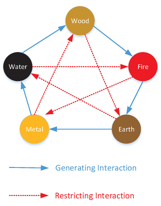
Figure 1. The generating and restricting interaction among five elements.

The Five-element Cycle Model (FECM) is founded upon the principles of the Five-element theory [22]. Consider a dynamic system comprising L elements. At time k, the force exerted on element ${\mathbf{x}}_i\left(k\right)$ by other elements is denoted as $F_i\left(k\right)$. Each element’s mass is represented by $m_i\left(k\right)$. The FECM is delineated as follows:

$$\left\{\begin{array}{c}\hfill F_i\left(k\right)={\omega }_{gp}ln\left[{\displaystyle \frac{m_{i-1}\left(k\right)}{m_i\left(k\right)}}\right]-{\omega }_{rp}ln\left[{\displaystyle \frac{m_{i-2}\left(k\right)}{m_i\left(k\right)}}\right]-\\ \hfill {\omega }_{ga}ln\left[{\displaystyle \frac{m_i\left(k\right)}{m_{i+1}\left(k\right)}}\right]-{\omega }_{ra}ln\left[{\displaystyle \frac{m_i\left(k\right)}{m_{i+2}\left(k\right)}}\right]& \\ \\ \hfill m_i(k+1)=m_i\left(k\right)\cdot {\displaystyle \frac{2}{1+exp(-F_i\left(k\right))}}\end{array}\right.$$

(7)

where $i=1,2,\dots ,L$. When $i=1$, $i-1$ is replaced by L; when $i=2$, $i-2$ is replaced by L; when $i=L$, $i+1$ is replaced by 1; when $i=L-1$, $i+2$ is replaced by 1. ${\omega }_{gp}$, ${\omega }_{rp}$, ${\omega }_{ga}$, and ${\omega }_{ra}$ are weight coefficients, typically set to 1.

2.3. Multi-Objective Five-Element Cycle Algorithm

Based on the FECM, the Five-element Cycle Optimization algorithm (FECO) is introduced [22]. Operating as an iterative algorithm, FECO tackles optimization problems, with each element representing a feasible solution. The population is divided into q cycles, each comprising L elements, as depicted in Figure 2. Typically, the objective function value of an element is equated to its mass. Leveraging the relationship between element masses and the forces exerted on them in the FECM, and higher forces correspond to smaller masses. Consequently, elements with greater forces are deemed superior solutions in optimization problems aimed at minimizing the objective function. This implies that as forces increase, element masses diminish, gradually converging towards the optimal solution. Hence, the force of each element dictates whether the solution is updated. Elements with lower forces, indicative of larger masses, necessitate updates to explore better solutions. Ultimately, the optimal solution is derived through iterative refinement.

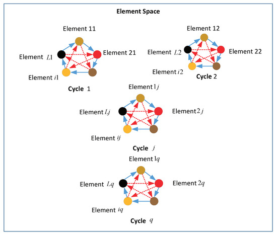
Figure 2. The structure of the element space.

The Multi-objective Five-element Cycle Optimization algorithm (MOFECO) is an extension of FECO tailored for addressing Multi-objective Optimization Problems (MOP) [24]. Given that MOP entails multiple objective functions, each element encompasses multiple forces. In [24], it is proposed that an element is retained in the iteration if at least two of its forces are positive; otherwise, the element undergoes an update. Conversely, in [25], an element is updated if the sum of forces across all its objective functions is negative.

3. Multi-Objective Five-Element Cycle Optimization Algorithm Based on Multi-Strategy Fusion for BITTP

3.1. Expression of Solution and Objective Function

The proposed Multi-objective Five-element Cycle Optimization algorithm based on Multi-strategy Fusion (MOFECO-MS) is utilized in this study to tackle the BITTP. In the context of MOFECO-MS applied to BITTP, each solution corresponds to an element within the FECM framework. The population, comprising N individuals of MOFECO-MS, is segmented into q cycles, each containing L elements. They are denoted as ${\mathbf{x}}_{ij}\left(k\right)$, an element representing the ith element in the jth cycle at the kth iteration, constituting a feasible solution for BITTP. The decision variables of BITTP encompass two components, the route plan ${\mathit{\pi }}_{ij}\left(k\right)$ and the item plan ${\mathbf{z}}_{ij}\left(k\right)$. The expression ${\mathbf{x}}_{ij}\left(k\right)=[{\mathit{\pi }}_{ij}\left(k\right),{\mathbf{z}}_{ij}\left(k\right)]$ succinctly captures this duality.

The route plan ${\mathit{\pi }}_{ij}\left(k\right)$ comprises n decision variables, corresponding to the number of cities, denoted as:

$${\mathit{\pi }}_{ij}\left(k\right)=[{\pi }_{1,ij}\left(k\right),{\pi }_{2,ij}\left(k\right),\cdots ,{\pi }_{n,ij}\left(k\right)]$$

(8)

The item plan ${\mathbf{z}}_{ij}\left(k\right)$ encompasses $n^{\prime }$ decision variables, representing the number of $n^{\prime }$ items, denoted as:

$${\mathbf{z}}_{ij}\left(k\right)=[z_{1,ij}\left(k\right),z_{2,ij}\left(k\right),\cdots ,{\mathrm{z}}_{n^{\prime },ij}\left(k\right)]$$

(9)

In MOFECO, the number of masses associated with each element is equivalent to the number of objective functions. Here, $m_{ij,r}\left(k\right)$ denotes the rth objective function value of the element ${\mathbf{x}}_{ij}\left(k\right)$:

$$m_{ij,r}\left(k\right)=f_r\left({\mathbf{x}}_{ij}\left(k\right)\right)$$

(10)

For BITTP, r takes values of 1 and 2.

Based on the relationship among FECM, MOFECO-MS, and BITTP as shown in Table 2, MOFECO-MS is designed to solve the BITTP. Table 2 illustrates the relationship between the Five-element Cycle Model (FECM), the Multi-objective Five-element Cycle Optimization algorithm (MOFECO-MS), and the Bi-objective Traveling Thief Problem (BITTP). In FECM, elements ${\mathbf{x}}_i\left(k\right)$ represent entities within the cycle, with mass $m_i\left(k\right)$ indicating their state, and force $F_i\left(k\right)$ reflecting the interactions driving system evolution.

Table 2. Relationship among FECM, MOFECO-MS and BITTP.

FECM	MOFECO-MS	BITTP
Elements ${\mathbf{x}}_i\left(k\right)(i=1,2,\cdots ,L)$	Elements ${\mathbf{x}}_{ij}\left(k\right)$ $(i=1,2,\cdots ,L;j=1,2,\cdots ,q)$	Solution (Tour plan, picking plan) ${\mathit{\pi }}_{ij}\left(k\right),{\mathbf{z}}_{ij}^k$
Mass of elements $m_i\left(k\right)$	Mass of elements $m_{ij,r}\left(k\right)(i=1,2,\cdots ,L;j=1,2,\cdots ,q;r=1,2)$	Objective functions (Travel time $f_1$ and Total profit $f_2$)
Force exerted on elements $F_i\left(k\right)$	Force exerted on elements $F_{ij,r}\left(k\right)$	Variables estimating the quality of solutions

In MOFECO-MS, these elements correspond to potential solutions within the algorithm’s population, where each element’s mass $m_{ij,r}\left(k\right)$ is linked to the objective function values in BITTP, indicating solution quality. The force $F_{ij,r}\left(k\right)$ applied to these elements represents the evolutionary pressure guiding the optimization process. The BITTP context translates these elements into concrete solutions (tour plans and picking plans), with their mass reflecting objective function values like travel time and total profit.

This table clarifies how MOFECO-MS leverages the principles of FECM, with each component in the optimization algorithm corresponding directly to the theoretical constructs in FECM, thereby providing a strong foundation for solving BITTP.

3.2. Initializing the Population

Since BITTP comprises two distinct components, addressing each component separately during the initial population construction phase is imperative. A sequence of n integers for the route plan is randomly generated, stipulating that the first integer corresponds to the starting city, denoted as city 1. Concurrently, the item plan is encoded using a binary scheme, where a value of 1 indicates the selection of an item, while 0 signifies its absence. During the initialization stage, we assume all items are initially selected, with subsequent adjustments performed using a repair operator. This repair operator ensures compliance with the knapsack capacity constraint by iteratively removing randomly selected items from the selection until the total weight of the chosen items conforms to the specified knapsack capacity. This iterative process continues until the cumulative weight of the selected items satisfies the knapsack capacity constraint. The pseudocode for the repair operator is presented in Algorithm 1.

Algorithm 1 Repair operator

Require:  Q, ${\mathbf{z}}_{ij}\left(k\right)$ Ensure:  ${\mathbf{z}}_{ij}\left(k\right)$ 1: $YesItems$⇐$find({\mathbf{z}}_{ij}\left(k\right)==1)$ 2: $restofWeight=Q-sum\left(weights\right(YesItems\left)\right)$ 3: while  $restofWeight<0$  do 4:     Randomly select one item t 5:     $z_{t,ij}\left(k\right)\leftarrow 0$ 6: end while 7: Return ${\mathbf{z}}_{ij}\left(k\right)$

After establishing the route and item plans, the objective function can be computed according to Section 2.1. Subsequently, the objective function value for each element can be assigned as their respective mass by (10).

3.3. Force Calculation

The number of forces exerted on element ${\mathbf{x}}_{ij}\left(k\right)$ by other elements in the jth cycle is equivalent to the number of objective functions. The rth force acting on ${\mathbf{x}}_{ij}\left(k\right)$ is denoted by $F_{ij,r}$ and computed using (11).

$$\begin{array}{cc}\hfill F_{ij,r}\left(k\right)& =ln\left[{\displaystyle \frac{m_{(i-1)j,r}\left(k\right)}{m_{ij,r}\left(k\right)}}\right]-ln\left[{\displaystyle \frac{m_{(i-2)j,r}\left(k\right)}{m_{ij,r}\left(k\right)}}\right]\hfill \\ \hfill & -ln\left[{\displaystyle \frac{m_{ij,r}\left(k\right)}{m_{(i+1)j,r}\left(k\right)}}\right]-ln\left[{\displaystyle \frac{m_{ij,r}\left(k\right)}{m_{(i+2)j,r}\left(k\right)}}\right]\hfill \end{array}$$

(11)

It can be seen from the above formula that the force of an element is closely related to its mass. The smaller the mass of an element is, the greater the force of the element is. Therefore, one can evaluate the element according to the force of each element.

3.4. Elements Sorting Strategy

In each iteration, it is essential to rank the elements for evaluation. Subsequently, we design the update strategy based on this ranking. Following the evaluation, we retain the elite elements while discarding the non-elite ones, ultimately identifying the optimal solutions.

In MOFECO-MS, we employ two sorting methods for these scenarios. Firstly, we sort the elements within each cycle based on their forces when determining the update strategy. Secondly, we utilize fast non-dominated sorting [26] to rank the elements according to their dominance relationship after each evolutionary iteration.

Since this paper entails two objective functions, each element possesses two distinct forces denoted as $F_{ij,r},r=1,2$. Consequently, unlike the single objective function scenario, the element with the greatest force cannot be straightforwardly deemed the optimal element within the cycle. Herein, we adopt a sorting approach where we initially arrange the forces $F_{ij,r},i=1,2,\cdots ,L,r=1,2$ in the jth cycle for each objective function in ascending order, yielding respective sequence numbers denoted as $temp$. Subsequently, we compute the sum of sequence numbers for each element across both objective functions. By sorting these sum values, we identify the element with the highest ranking within cycle j, denoted as ${\mathbf{x}}_{i_{b}j}$. We collate all ${\mathbf{x}}_{i_{b}j},j=1,2,\cdots ,q$ into $po{p}_{bc}$, structured as $po{p}_{bc}=[{\mathbf{x}}_{i_{b}1},{\mathbf{x}}_{i_{b}2},\cdots ,{\mathbf{x}}_{i_{b}t},\cdots ,{\mathbf{x}}_{i_{b}q}]$. $po{p}_{bc}$ encompasses two element types: those within the same cycle as ${\mathbf{x}}_{ij}$, termed ${\mathbf{x}}_{bj}$, and those outside cycle j, denoted as ${\mathbf{x}}_{b{j}^{\prime }}$. This sorted collection is denoted as $popsort$. The comprehensive sorting process is delineated in Algorithm 2.

Algorithm 2 The sorting process of the elements in each cycle

Require:  $pop,F_{ij,r},i=1,2,\cdots ,L,j=1,2,\cdots ,q,r=1,2$ Ensure:  ${pop}_{sort},{pop}_{bc}$ 1: $temp$⇐$zeros(L,2)$ 2: for  $j=1\to q$  do 3:     $[\sim ,noF]$⇐$Sort\left(F_{ij,r}\right),$ 4:     for $r=1\to 2$ do 5:         for $i=1\to L$ do 6:            $temp\left(noF\right(i,r),r)$⇐i 7:         end for 8:     end for 9:     $[,no]$⇐$Sort\left(sum\right(temp,2\left)\right)$ 10:     $i_b$⇐$no\left(L\right)$ 11:     ${pop}_{bc}\left(j\right)$⇐ ${\mathbf{x}}_{i_{b}j}$ 12:     ${pop}_{sort}((j-1)\times L+1:(j-1)\times L+L,:)$⇐ $pop(no,:)$ 13: end for 14: Return $po{p}_{sort}$, ${pop}_{bc}$

Once the elements are sorted, we can identify the optimal element within each cycle based on the force order. Additionally, employing non-dominated sorting enables us to pinpoint the Pareto optimal solution, representing the solution with a non-dominant sorting rank of 1 [26] as the current optimal solution.

Hence, elements can be categorized into different types, as illustrated in Table 3.

Table 3. Symbols and description of the elements.

Symbols	Description
${\mathbf{x}}_{ij}\left(k\right)$	The element to be updated
${\mathbf{x}}_{bj}\left(k\right)$	The best element in the cycle j
${\mathbf{x}}_{b{j}^{\prime }}\left(k\right)$	The best element in any of the $q-1$ cycles except the cycle j
${\mathbf{x}}_{aps}\left(k\right)$	Any element in the current optimal solution set

3.5. Exploration Strategy

The exploration rate represents the likelihood of an intelligent optimization algorithm selecting new solutions for exploration. A higher exploration rate implies a greater inclination of the algorithm towards exploring uncharted solution spaces, thereby increasing the chances of discovering optimal solutions. MOFECO-MS employs the crossover operator to enhance the algorithm’s exploration capability. Since the decision variables of BITTP consist of two parts, the route plan and the item plan, these two components are separately updated during element updates.

For the route plan, the partial mapping crossover operator (PMX) [27] is employed because it maintains population diversity and prevents the algorithm from converging to local optima. PMX facilitates diversity preservation by avoiding the generation of duplicate genes through mapping, thus enhancing both convergence and exploration capabilities.

As the item plan is binary encoded, the uniform crossover operator [28] is utilized. This operator exchanges genes at each locus of paired individuals with the same crossover probability, generating two new individuals. Uniform crossover enhances population diversity, facilitates gene communication and combination, and improves the algorithm’s search efficiency and convergence rate.

During the exploration phase, expanded and narrowed exploration strategies are employed to expedite and enhance the search process. Expanded exploration involves crossing element ${\mathbf{x}}_{ij}\left(k\right)$ with the best element in each cycle, comprising ${\mathbf{x}}_{bj}\left(k\right)$ and ${\mathbf{x}}_{b{j}^{\prime }}\left(k\right)$. On the other hand, narrowed exploration entails crossing ${\mathbf{x}}_{ij}\left(k\right)$ with ${\mathbf{x}}_{aps}\left(k\right)$, with the frequency of these methods adjusted by probability $p_c$. The pseudocode for the exploration phase is depicted in Algorithm 3. Notably, the probability of expanded exploration is $p_c$, while the probability of narrowed exploration is $1-p_c$.

Algorithm 3 Exploration phase

Require:  ${\mathbf{x}}_{ij}\left(k\right)$, ${\mathbf{x}}_{i_{b}t}\left(k\right),t=1,2,\cdots ,q$, ${\mathbf{x}}_{aps}\left(k\right)$ Ensure:  ${\mathbf{x}}_{new}\left(k\right)$ 1: if $rand<p_c$⊳ $rand$ is a random number between 0-1 then 2:     ${\mathbf{x}}_{new}\left(k\right)$⇐$\mathtt{Croc}({\mathbf{x}}_{ij}\left(k\right),{\mathbf{x}}_{i_{b}t}\left(k\right))$ 3: else 4:     ${\mathbf{x}}_{new}\left(k\right)$⇐$\mathtt{Croc}({\mathbf{x}}_{ij}\left(k\right),{\mathbf{x}}_{aps}\left(k\right))$ 5: end if 6: Return ${\mathbf{x}}_{new}\left(k\right)$

3.6. Exploitation Strategy

The exploitation rate, within the context of intelligent optimization algorithms, signifies the likelihood or frequency of leveraging known high-quality solutions. A higher exploitation rate implies a greater propensity for utilizing established reasonable solutions with the anticipation of further optimization around them. Typically, this rate is achieved by selecting the best solution or weighting the selection based on solution quality. While a higher exploitation rate aids rapid convergence towards local optima, it also raises the risk of entrapment in local optima, potentially overlooking the global optimum. Hence, selecting the appropriate exploitation strategy is crucial.

MOFECO-MS utilizes a mutation operator to enhance exploitation capability, similar to the crossover operator. This mutation operator is bifurcated into two segments: mutation of the route plan and mutation of the item plan. For the route plan, we employ the swap operator [29]; for the item plan, we introduce a novel heuristic operator proposed in this paper.

Within the heuristic operator, the first step involves computing the remaining knapsack capacity, denoted as $restofWeight$. Subsequently, we identify those whose weights are lower than the remaining knapsack capacity from the untaken items. Next, randomly select an item meeting the weight criteria and place it into the knapsack to augment profit. The pseudocode outlining the heuristic operator is delineated in Algorithm 4.

Algorithm 4 Heuristic operator

Require:  Q, ${\mathbf{z}}_{ij}\left(k\right),weights$ Ensure:  ${\mathbf{z}}_{ij}\left(k\right)$ 1: $YesItems$⇐$find({\mathbf{z}}_{ij}\left(k\right)==1)$ 2: $restofWeight=Q-sum\left(weights\right(YesItems\left)\right)$ 3: $NoItems$⇐$find({\mathbf{z}}_{ij}\left(k\right)==0)$ 4: $Am$⇐$find(restofWeight>weights(NoItems\left)\right)$ 5: if  $Am\ne \varnothing$  then 6:     Randomly select one item t from $Am$ 7:     $z_{t,ij}\left(k\right)\leftarrow 1$ 8: end if 9: Return ${\mathbf{z}}_{ij}\left(k\right)$

Indeed, the exploitation phase is also segregated into expanded and narrowed exploitation. Expanded exploitation involves mutating any of the current optimal elements ${\mathbf{x}}_{aps}\left(k\right)$, while narrowed exploitation entails mutating an element that is potentially a good solution in the exploitation phase, represented by ${\mathbf{x}}_{gs}\left(k\right)$. The frequency of expanded and narrowed exploitation is determined by the probability $p_m$. The pseudocode outlining the exploitation phase is depicted in Algorithm 5. Notably, the probability of expanded exploitation is $p_m$, while the probability of narrowed exploitation is $1-p_m$.

Algorithm 5 Exploitation phase

Require:  ${\mathbf{x}}_{gs}\left(k\right)$, ${\mathbf{x}}_{aps}\left(k\right)$, Ensure:  ${\mathbf{x}}_{new}\left(k\right)$ 1: if  $rand<p_m$  then 2:     ${\mathbf{x}}_{new}\left(k\right)$⇐$\mathtt{Mut}\left({\mathbf{x}}_{aps}\left(k\right)\right)$ 3: else 4:     ${\mathbf{x}}_{new}\left(k\right)$⇐$\mathtt{Mut}\left({\mathbf{x}}_{gs}\left(k\right)\right)$ 5: end if 6: Return ${\mathbf{x}}_{new}\left(k\right)$

3.7. Elite Retention Strategy

The elite retention strategy is a commonly employed technique to modulate the progression rate of algorithms. Throughout the iterative process of the algorithm delineated in this paper, select individuals showcasing superior performance are preserved to impede their elimination, thereby expediting the algorithm’s convergence. After each iteration, the parent and offspring populations undergo reorganization to safeguard exceptional individuals from elimination, thereby realizing elite retention.

3.8. Update Strategy for the Element

The element update strategy significantly influences the algorithm’s performance. Therefore, the crucial issues we need to address revolve around which elements necessitate updating and how to enact those updates.

Given the elitist strategy we employ, which preserves the entire parent population, during element updates, we can update each element to explore as many new individuals as possible, thereby hastening the discovery of the global optimal solution.

In the proposed algorithm, we initially employ the aforementioned element sorting strategy, ensuring that elements within each cycle are arranged from worst to best, as illustrated in Figure 3. Subsequently, we implement exploration capability with the first l elements and exploitation with the last $L-l$ elements in each cycle. The pseudocode detailing this process is provided in Algorithm 6.

Algorithm 6 The update process for elements

Require:  ${\mathbf{x}}_{ij}\left(k\right)$ Ensure:  ${\mathbf{x}}_{new}\left(k\right)$ 1: for  $j=1\to q$  do 2:     for $i=1\to L$ do 3:         if $i\le l$ then 4:            Enter the exploration phase 5:         else 6:            Enter the exploitation phase 7:         end if 8:     end for 9: end for 10: Return ${\mathbf{x}}_{new}\left(k\right)$

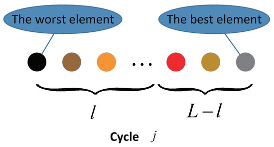
Figure 3. The L elements sorted from the worst to the best in the cycle j.

When selecting the first l elements in each cycle for exploration, we update these l elements using the exploration strategy.

During the exploration phase, ${\mathbf{x}}_{i_{b}t}\left(k\right)$ denotes the best element in the cycle, encompassing both ${\mathbf{x}}_{bj}\left(k\right)$ within the same cycle j as ${\mathbf{x}}_{ij}\left(k\right)$, as well as ${\mathbf{x}}_{b{j}^{\prime }}\left(k\right)$, which represents the best element among the remaining $q-1$ cycles.

Conversely, we adopt the exploitation strategy to exploit the last $L-l$ elements because these elements have been sorted within the cycle and are deemed superior solutions. Thus, in the exploitation phase, ${\mathbf{x}}_{gs}\left(k\right)$ comprises the optimal elements within cycle ${\mathbf{x}}_{bj}\left(k\right)$, ${\mathbf{x}}_{b{j}^{\prime }}\left(k\right)$, and the updated elements ${\mathbf{x}}_{ij}\left(k\right)$.

To determine the most effective search method for updating elements, we devised four distinct combinations, denoted as SM1–SM4, outlined in Table 4.

Table 4. Search methods in updating.

	Expanded Exploration	Narrowed Exploration	Expanded Exploitation	Narrowed Exploitation
	$p_c$	$1-p_c$	$p_m$	$1-p_m$
SM1	$\mathtt{Croc}({\mathbf{x}}_{ij}\left(k\right),{\mathbf{x}}_{bj}\left(k\right))$	$\mathtt{Croc}({\mathbf{x}}_{ij}\left(k\right),{\mathbf{x}}_{aps}\left(k\right))$	$\mathtt{Mut}\left({\mathbf{x}}_{aps}\left(k\right)\right)$	$\mathtt{Mut}\left({\mathbf{x}}_{bj}\left(k\right)\right)$
SM2	$\mathtt{Croc}({\mathbf{x}}_{ij}\left(k\right),{\mathbf{x}}_{bj}\left(k\right))$	$\mathtt{Croc}({\mathbf{x}}_{ij}\left(k\right),{\mathbf{x}}_{aps}\left(k\right))$	$\mathtt{Mut}\left({\mathbf{x}}_{aps}\left(k\right)\right)$	$\mathtt{Mut}\left({\mathbf{x}}_{ij}\left(k\right)\right)$
SM3	$\mathtt{Croc}({\mathbf{x}}_{ij}\left(k\right),{\mathbf{x}}_{bj}\left(k\right))$	$\mathtt{Croc}({\mathbf{x}}_{ij}\left(k\right),{\mathbf{x}}_{aps}\left(k\right))$	$\mathtt{Mut}\left({\mathbf{x}}_{aps}\left(k\right)\right)$	$\mathtt{Mut}\left({\mathbf{x}}_{b{j}^{\prime }}\left(k\right)\right)$
SM4	$\mathtt{Croc}({\mathbf{x}}_{ij}\left(k\right),{\mathbf{x}}_{b{j}^{\prime }}\left(k\right))$	$\mathtt{Croc}({\mathbf{x}}_{ij}\left(k\right),{\mathbf{x}}_{aps}\left(k\right))$	$\mathtt{Mut}\left({\mathbf{x}}_{aps}\left(k\right)\right)$	$\mathtt{Mut}\left({\mathbf{x}}_{b{j}^{\prime }}\left(k\right)\right)$

In Table 4, the variations among the three sets of methods, SM1, SM2, and SM3, lie in the selection of elements ${\mathbf{x}}_{gs}\left(k\right)$ during narrowed exploitation. Specifically, they are ${\mathbf{x}}_{bj}\left(k\right)$, ${\mathbf{x}}_{ij}\left(k\right)$, and ${\mathbf{x}}_{b{j}^{\prime }}\left(k\right)$, respectively. The distinction between SM3 and SM4 pertains to the choice of $\mathbf{x}{i}_{b}t\left(k\right)$ for exploration during expanded exploration, which are ${\mathbf{x}}_{bj}\left(k\right)$ and ${\mathbf{x}}_{b{j}^{\prime }}\left(k\right)$, respectively.

3.9. Flowchart of MOFECO-MS

The flowchart depicting the MOFECO-MS algorithm is presented in Figure 4. Notably, the parameter $c_{max}$ employed in the initialization phase denotes the maximum number of objective function computations and serves as the termination criterion for the algorithm. From this flowchart, it is evident that the operators used in our proposed algorithm are genetic operators, such as crossover and mutation.

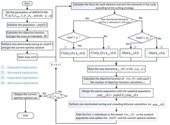
Figure 4. The flowchart of Multi-objective Five-element Cycle Optimization algorithm based on Multi-strategy Fusion (MOFECO-MS).

While MOFECO-MS shares several similarities with traditional genetic algorithms (GAs) in terms of using these genetic operators and following an iterative process, there are key differences that distinguish it. In MOFECO-MS, the population is organized into cycles (or rings) as defined by the Five-element Cycle Model, where each element corresponds to an individual in a GA. The entire set of cycles represents the population, and genetic operators are applied based on the sorting of elements within each cycle, rather than through the selection mechanisms typical in GAs. This cyclic ordering, driven by the Five-element Cycle, governs how elements are updated, ensuring that the process aligns with the model’s inherent dynamics. This approach not only maintains a balance between exploration and exploitation but also introduces a novel mechanism that differentiates MOFECO-MS from conventional GAs.

4. Experimental Setup

4.1. Operating Environment

In this study, we conducted a series of computational experiments to assess the effectiveness of the proposed algorithm. The implementation of these experiments was carried out using MATLAB R2018a and the computational experiments were executed on a high-performance system equipped with a 2.4 GHz Intel Xeon E5645 processor (Intel, Santa Clara, CA, USA). The system also featured 32 GB of RAM, providing ample memory to handle large datasets and complex calculations efficiently. The operating environment for these experiments was Windows 10. This setup ensured that the experiments were performed in a stable and efficient computing environment, thereby allowing for accurate and reliable evaluation of the algorithm’s performance.

4.2. BITTP Instances

The test instances utilized in this paper are drawn from the comprehensive BITTP benchmark developed by Polyakovskiy et al. [23]. Specifically, we have selected nine instances with varying numbers of cities and items, as detailed in Table 5. These instances cover a range of scenarios with varying numbers of cities and items, providing a robust assessment of the proposed algorithm’s performance across different problem scales and complexities.

Table 5. The Bi-objective Traveling Thief Problem (BITTP) test instances.

Instance	${\mathit{n}}^{\prime }$	Q	Knapsack Type	R
$eil{51}_{\text{\_}}n50$	50	4029	bsc	01
$eil51\text{\_}n250$	250	22,832	usw	05
$eil51\text{\_}n500$	500	22,486	unc	10
$ch150\text{\_}n149$	149	12,310	bsc	01
$ch150\text{\_}n1395$	745	68,034	usw	05
$ch150\text{\_}n1490$	1490	1,262,022	unc	10
$a280\text{\_}n279$	279	25,936	bsc	01
$a280\text{\_}n1395$	1395	637,010	usw	05
$a280\text{\_}n2790$	2790	1,262,022	unc	10

Table 5 outlines the key characteristics of the selected instances. The instances are defined by the number of cities (n), the number of items ($n^{\prime }$), and the knapsack capacity (Q). The knapsack component of each instance is constructed based on the ratio of item profit to weight, categorized into three distinct types: bounded strongly correlated (bsc), uncorrelated with similar weights (usw), and uncorrelated (unc). The column labeled R indicates the distribution of items across cities, with the number in each city excluding the departure city where no items are available.

4.3. The Statistical Analysis Methods

The statistical analysis methods are based on the computational and experimental outcomes derived from 15 independent runs of each algorithm. Specifically, the reported results include the best solution (Best), worst solution (Worst), median (Median), mean (Average), and standard deviation (StdDev) obtained across these 15 runs. Here, is a detailed explanation of each statistical indicator:

• Best: This represents the best performance achieved by the algorithm across the 15 runs. It indicates the highest level of performance that the algorithm can reach under the given experimental conditions. A higher best value generally suggests that the algorithm is capable of finding very high-quality solutions, even if it is not consistent every time.
• Worst: This represents the worst performance observed among the 15 runs. It provides insight into the least favorable outcome that the algorithm might produce. A higher worst value is preferable as it indicates that even in the least favorable scenario, the algorithm still performs relatively well.
• Median: This is the middle value of the performance results when they are sorted in ascending order. It gives an indication of the typical performance of the algorithm, minimizing the impact of outliers. The median is particularly useful in understanding the central tendency of the algorithm’s performance.
• Mean (Average): This represents the mean performance across all 15 runs. It is calculated by summing all the performance values and dividing by the number of runs. The average provides a general idea of the algorithm’s overall performance.
• Standard Deviation (StdDev): This measures the amount of variation or dispersion in the performance results. A lower standard deviation is preferable as it indicates that the algorithm’s performance is more consistent across different runs. This means that the algorithm is reliably achieving similar results, which is a desirable characteristic in optimization algorithms.

Each of these statistical indicators provides a different perspective on the algorithm’s performance. By considering them together, we can gain a comprehensive understanding of the strengths and limitations of each algorithm under different conditions. The performance metrics are chosen to ensure that the analysis is thorough and that the best algorithm can be identified based on a balanced consideration of all relevant factors.

4.4. Performance Metrics

Multi-objective optimization (MOO) algorithms are designed to solve problems with multiple conflicting objectives, where the goal is to find a set of solutions that optimally balance these objectives. Evaluating the performance of MOO algorithms is crucial for assessing their effectiveness in finding high-quality solutions across the entire Pareto front, the set of non-dominated solutions.

In this paper, we take the Hypervolume (HV), Spacing (SP), and Pure Diversity (PD) metrics together as evaluation criteria to evaluate the performance of algorithms. Choosing the HV, SP, and PD metrics together provides a comprehensive assessment of the algorithm’s performance across different aspects:

HV assesses both convergence and overall spread, SP ensures even distribution of solutions, and PD guarantees exploration of the entire search space. These metrics collectively ensure that the algorithm is not only converging to the optimal solutions but also maintaining a diverse set of solutions. This balance is critical in multi-objective optimization as it provides a set of well-distributed, high-quality solutions for decision-makers.

By considering all three metrics, we can gain a complete understanding of the algorithm¡¯s strengths and weaknesses in solving multi-objective optimization problems, leading to more informed decisions in algorithm selection and development. Here, is a detailed description of them:

4.4.1. Hypervolume (HV)

Hypervolume (HV) serves as a comprehensive indicator for assessing multi-objective evolutionary algorithms, capable of concurrently reflecting the convergence and distribution characteristics of the algorithm [30]. It is computed by determining the hypervolume of the region bounded by the Pareto front and the reference point. The calculation formula is provided below:

$$HV=\lambda \left(\bigcup _{i=1}^{\left|s\right|}{\upsilon }_i\right)$$

(12)

where $\lambda$ denotes the Lebesgue measure, ${\upsilon }_i$ signifies the hypervolume formed by the reference point $Ref$ and a point on the Pareto front, and s denotes the Pareto front generated by the algorithm.

In selecting the reference point $Ref$, we use the worst value of each objective function observed on the Pareto front. Hence, a larger hypervolume ($HV$) corresponds to superior algorithm performance.

4.4.2. Spacing (SP)

The spacing (SP) metric is a widely used measure in MOO to assess the uniformity of the distribution of solutions in the Pareto front. It evaluates how evenly the solutions are spread along the Pareto front. A lower value of SP indicates a more uniformly distributed set of solutions, which is desirable in MOO as it ensures better coverage and diversity [31]. The SP metric is calculated using the following steps and formula:

• Calculate the distance:
  For each solution i in the obtained Pareto front, compute the distance $d_i$ to its nearest neighbor solution in the objective space. This distance is typically calculated using the Euclidean distance.

  $$d_i=\underset{j\ne i}{min}\sqrt{\sum _{k=1}^M{\left(f_k\left(x_i\right)-f_k\left(x_j\right)\right)}^2}$$

  (13)

  –

  M is the number of objectives,

  –

  $f_k\left(x_i\right)$ is the value of the k-th objective for solution $x_i$,

  –

  $f_k\left(x_j\right)$ is the value of the k-th objective for solution $x_j$.

• Compute the average distance:
  Calculate the average of these minimum distances.

  $$\overline{d}={\displaystyle \frac{1}{\left|A\right|}}\sum _{i=1}^{\left|A\right|}{d}_i$$

  (14)

  where A is the Pareto front. $\left|A\right|$ is the number of solutions in the Pareto front.
• Calculate the SP metric:
  Finally, compute the SP metric as the standard deviation of the distances $d_i$ from their mean $\overline{d}$.

  $$SP=\sqrt{{\displaystyle \frac{1}{\left|A\right|-1}}\sum _{i=1}^{\left|A\right|}{(d_i-\overline{d})}^2}$$

  (15)

By using the SP metric, we can quantitatively evaluate and compare the distribution quality of solution sets obtained by different multi-objective optimization algorithms. Lower SP indicates that the solutions are more evenly distributed along the Pareto front, which is desirable. Higher SP indicates uneven distribution of solutions, suggesting gaps or clusters in the Pareto front.

4.4.3. Pure Diversity (PD)

In multi-objective optimization algorithms, the PD metric is used to assess the diversity of a solution set generated by the algorithm, focusing on the differences between the solutions [32]. This metric is important for understanding the algorithm’s ability to explore the solution space comprehensively. Here, is a common formula for calculating $PD$:

$$PD={\displaystyle \frac{2}{\left|A\right|\left(\right|A|-1)}}\sum _{i=1}^{\left|A\right|-1}\sum _{j=i+1}^{\left|A\right|}d\left({\mathbf{x}}_i,{\mathbf{x}}_j\right)$$

(16)

where

• ${\mathbf{x}}_i,{\mathbf{x}}_j$ are two different solutions from the set,
• $d\left({\mathbf{x}}_i,{\mathbf{x}}_j\right)$ is the distance between these two solutions, which can be calculated using the Euclidean distance or another suitable metric.

This formula calculates the average distance between all possible pairs of solutions in the set, providing a measure of the set’s diversity. A higher value indicates better diversity, meaning greater differences between the solutions.

5. Experimental Results and Analysis

5.1. Parameter Setting of MOFECO-MS

In the MOFECO-MS algorithm, several parameters require optimization, including the population size N, the termination conditions of the algorithm $c_{max}$, the crossover probability $p_c$, mutation probability $p_m$ for updating elements, the number of cycles q, the number of elements L allocated in each cycle, and the parameter l determining the ratio of exploration to exploitation within each cycle. To identify the optimal values for these parameters, we conducted experiments individually for each parameter, all performed on the $a280\text{\_}n279$ instance and each set of experiments was run 15 times independently.

5.1.1. Determining the Parameters N and $c_{max}$

To facilitate a more equitable comparison with other optimization algorithms, we have set the termination criterion for our iterative algorithm, MOFECO-MS, not by the number of iterations but by the number of objective function evaluations. Since different optimization algorithms employ varying update strategies at each iteration, using the number of objective function evaluations as the termination criterion ensures a fairer comparison.

Therefore, under this termination condition, we set the number of iterations to a relatively large value to accommodate the required number of objective function evaluations. The number of objective function evaluations is determined based on the population size. The population size settings were referenced from [22], and we configured different N and corresponding $c_{max}$ values, as shown in Table 6.

Table 6. Evaluation of N and $c_{max}$ on performance metrics.

N	${\mathit{c}}_{\mathbf{max}}$	${\mathbf{HV}}_{\mathbf{Ave}}$	t
50	500 × N	1.23 × ${10}^{11}$	35.18
50	1000 × N	1.46 × ${10}^{11}$	76.46
50	2000 × N	1.53 × ${10}^{11}$	187.01
100	500 × N	1.94 × ${10}^{11}$	71.02
100	1000 × N	2.98 × ${10}^{11}$	155.75
100	2000 × N	3.05 × ${10}^{11}$	365.49
200	500 × N	1.81 × ${10}^{11}$	175.31
200	1000 × N	2.88 × ${10}^{11}$	357.59
200	2000 × N	5.65 × ${10}^{11}$	895.15

Table 6 presents the results of experiments conducted with different combinations of N and $c_{max}$. The performance metrics considered are the average hypervolume $H{V}_{Ave}$ and the computation time t.

The combination of $N=100$, $c_{max}$ = 1000 × N was selected in Table 6 due to its superior performance across the metrics. Specifically:

• Hypervolume ($H{V}_{Ave}$): The average hypervolume value of 2.98 × ${10}^{11}$ indicates a high-quality solution set, demonstrating better convergence and diversity compared to other configurations.
• Computation time (t): With a computation time of 155.75, this configuration offers a reasonable balance between solution quality and computational efficiency. While there are configurations with slightly higher hypervolume values, they require significantly more computation time, making $N=100$, $c_{max}$ = 1000 × N the most efficient choice overall.

In addition, Figure 5 shows Pareto fronts under different N while keeping $c_{max}$ = 500 × N. The Pareto fronts are generated by running the algorithm 15 times, with the HV metric taken as the median value. Among the tested values of $N(50,100,200)$, $N=100$ is chosen because it likely provides a good balance between convergence speed and solution quality, as indicated by the Pareto front.

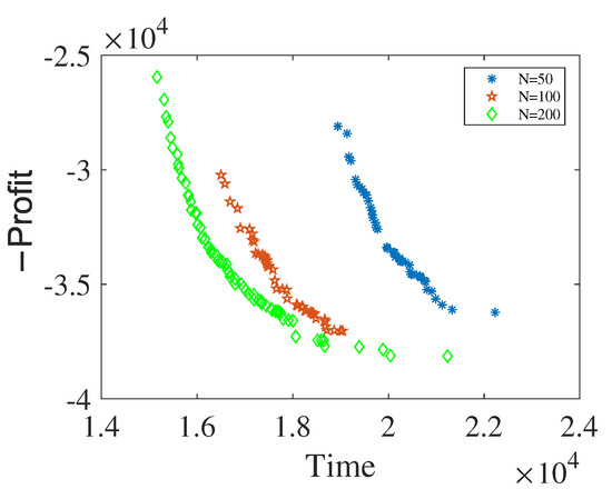
Figure 5. Pareto fronts under different N.

Figure 6 shows Pareto fronts under different $c_{max}$ with $N=100$. The Pareto fronts are generated by varying $c_{max}$. By observing the Pareto fronts, $c_{max}$ = 1000 × N is selected because it demonstrates a better trade-off between the objective functions (in this case, profit and time). The chosen $c_{max}$ value ensures that the algorithm can effectively explore the solution space and find optimal solutions.

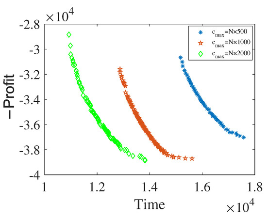
Figure 6. Pareto fronts under different $c_{max}$.

Therefore, by selecting this combination, we ensure that our algorithm achieves high-quality solutions within a manageable computational budget, thereby providing a robust and efficient optimization framework.

5.1.2. Determining the Parameters $p_c$ and $p_m$

Table 7 provides a concise nomenclature for the MOFECO-MS algorithm corresponding to different combinations of $p_c$ and $p_m$. For instance, $p_{cm1}$ denotes the algorithm with $p_c=0.9$ and $p_m=0.9$.

Table 7. Algorithm names with different $p_c$ and $p_m$.

	${\mathit{p}}_{\mathit{c}}=0.9$	${\mathit{p}}_{\mathit{c}}=0.5$	${\mathit{p}}_{\mathit{c}}=0.1$
$p_m=0.9$	$p_{cm1}$	$p_{cm4}$	$p_{cm7}$
$p_m=0.5$	$p_{cm2}$	$p_{cm5}$	$p_{cm8}$
$p_m=0.1$	$p_{cm3}$	$p_{cm6}$	$p_{cm9}$

Table 8 presents the experimental outcomes for various $p_c$ and $p_m$ values. We emphasize the algorithms exhibiting the best results for each performance metric. Notably, algorithm $p_{cm1}$ almost demonstrates superior performance across all metrics. Consequently, we conclude that $p_c=0.9$ and $p_m=0.9$ yield optimal results. Furthermore, we conduct verification tests for specific $p_c$ and $p_m$ values, as shown in Table 9 and Table 10. Once again, the results reaffirm the superiority of $p_c=0.9$ and $p_m=0.9$.

Table 8. Statistical results of HV indicator of the algorithms for different $p_c$, $p_m$.

	Best	Worst	Median	Average	StdDev
$p_{cm1}$	3.25 × ${10}^{11}$	2.79 × ${10}^{11}$	2.93 × ${10}^{11}$	2.98 × ${10}^{11}$	1.25 × ${10}^{10}$
$p_{cm2}$	3.04 × ${10}^{11}$	1.01 × ${10}^{11}$	2.33 × ${10}^{11}$	2.36 × ${10}^{11}$	5.86 × ${10}^{10}$
$p_{cm3}$	2.91 × ${10}^{11}$	1.50 × ${10}^{11}$	2.60 × ${10}^{11}$	2.35 × ${10}^{11}$	5.96 × ${10}^{10}$
$p_{cm4}$	3.25 × ${10}^{11}$	1.66 × ${10}^{11}$	1.95 × ${10}^{11}$	2.25 × ${10}^{11}$	6.38 × ${10}^{10}$
$p_{cm5}$	3.05 × ${10}^{11}$	1.91 × ${10}^{11}$	2.69 × ${10}^{11}$	2.55 × ${10}^{11}$	5.21 × ${10}^{10}$
$p_{cm6}$	3.08 × ${10}^{11}$	2.13 × ${10}^{11}$	2.71 × ${10}^{11}$	2.64 × ${10}^{11}$	3.70 × ${10}^{10}$
$p_{cm7}$	3.39 × ${10}^{11}$	2.31 × ${10}^{11}$	2.92 × ${10}^{11}$	2.92 × ${10}^{11}$	4.02 × ${10}^{10}$
$p_{cm8}$	3.16 × ${10}^{11}$	1.32 × ${10}^{11}$	1.57 × ${10}^{11}$	2.12 × ${10}^{11}$	9.27 × ${10}^{10}$
$p_{cm9}$	3.39 × ${10}^{11}$	2.31 × ${10}^{11}$	2.92 × ${10}^{11}$	2.92 × ${10}^{11}$	4.02 × ${10}^{10}$

Table 9. Algorithm names with special $p_c$ and $p_m$.

	${\mathit{p}}_{\mathit{c}}=0$	${\mathit{p}}_{\mathit{c}}=1$
$p_m=0$	$s{p}_{cm1}$	$s{p}_{cm3}$
$p_m=1$	$s{p}_{cm2}$	$s{p}_{cm4}$

Table 10. Statistical results of HV indicator of the algorithm using special $p_c$, $p_m$.

	Best	Worst	Median	Average	StdDev
$s{p}_{cm1}$	3.11 × ${10}^{11}$	1.35 × ${10}^{11}$	1.93 × ${10}^{11}$	2.18 × ${10}^{11}$	8.71 × ${10}^{10}$
$s{p}_{cm2}$	3.32 × ${10}^{11}$	1.83 × ${10}^{11}$	2.07 × ${10}^{11}$	2.34 × ${10}^{11}$	6.00 × ${10}^{10}$
$s{p}_{cm3}$	2.78 × ${10}^{11}$	1.31 × ${10}^{11}$	1.88 × ${10}^{11}$	1.94 × ${10}^{11}$	5.66 × ${10}^{10}$
$s{p}_{cm4}$	2.89 × ${10}^{11}$	1.87 × ${10}^{11}$	2.22 × ${10}^{11}$	2.33 × ${10}^{11}$	4.79 × ${10}^{10}$

5.1.3. Determining the Parameters L and q

Since this paper employs element sorting within cycles, parameter variations q and L significantly influence the algorithm’s performance. Table 11 presents the outcomes corresponding to four distinct combinations of q and L. Notably, the analysis indicates superior performance when $L=5$ and $q=20$. Consequently, we opt to set $L=5$ and $q=20$ accordingly.

Table 11. Statistical results of HV indicator of the algorithms with different L and q.

	Best	Worst	Median	Average	StdDev
$L=5,q=20$	3.25 × ${10}^{11}$	2.79 × ${10}^{11}$	2.93 × ${10}^{11}$	2.98 × ${10}^{11}$	1.25 × ${10}^{10}$
$L=10,q=10$	3.07 × ${10}^{11}$	9.97 × ${10}^{10}$	1.80 × ${10}^{11}$	2.06 × ${10}^{11}$	8.21 × ${10}^{10}$
$L=20,q=5$	2.85 × ${10}^{11}$	1.63 × ${10}^{11}$	2.48 × ${10}^{11}$	2.34 × ${10}^{11}$	5.04 × ${10}^{10}$
$L=50,q=2$	2.85 × ${10}^{11}$	1.63 × ${10}^{11}$	2.48 × ${10}^{11}$	2.34 × ${10}^{11}$	5.04 × ${10}^{10}$

5.1.4. Determining the Parameter l

After determining $L=5$, we ascertain the optimal value for l. Based on the experimental findings showcased in Table 12, it becomes evident that the algorithm yields superior results when $l=3$.

Table 12. Statistical results of HV indicator of the algorithms with different l.

l	Best	Worst	Median	Average	StdDev
1	1.32 × ${10}^{11}$	7.01 × ${10}^{10}$	1.16 × ${10}^{11}$	1.11 × ${10}^{11}$	2.39 × ${10}^{10}$
2	1.83 × ${10}^{11}$	5.76 × ${10}^{10}$	1.78 × ${10}^{11}$	1.43 × ${10}^{11}$	5.43 × ${10}^{10}$
3	3.25 × ${10}^{11}$	2.79 × ${10}^{11}$	2.93 × ${10}^{11}$	2.98 × ${10}^{11}$	1.25 × ${10}^{10}$
4	2.81 × ${10}^{11}$	2.34 × ${10}^{11}$	2.71 × ${10}^{11}$	2.61 × ${10}^{11}$	1.97 × ${10}^{10}$

5.2. Selection of Search Methods

In Section 3.8, we outline the design of four distinct search methods to select elements for element updates. Subsequently, we conduct experiments to compare the performance of these four methods and identify the most effective one for integration into the final MOFECO-MS.

For experimentation purposes, we fix the parameters as follows: $L=5$, $q=20$, $l=L\times 60\%$, $p_c=0.9$, $p_m=0.9$, $N=100$ and $c_{max}=N\times 1000$. We select the instance $a280\text{\_}n279$ for testing to identify the optimal method for updating elements. The experimental findings are summarized in Table 13.

Table 13. Statistical results of HV indicator obtained by four different search methods.

	Best	Worst	Median	Average	StdDev
SM1	2.99 × ${10}^{11}$	1.62 × ${10}^{11}$	2.36 × ${10}^{11}$	2.26 × ${10}^{11}$	4.99 × ${10}^{10}$
SM2	2.99 × ${10}^{11}$	1.49 × ${10}^{11}$	2.31 × ${10}^{11}$	2.29 × ${10}^{11}$	5.00 × ${10}^{10}$
SM3	3.11 × ${10}^{11}$	2.07 × ${10}^{11}$	2.56 × ${10}^{11}$	2.61 × ${10}^{11}$	3.09 × ${10}^{10}$
SM4	3.25 × ${10}^{11}$	2.79 × ${10}^{11}$	2.93 × ${10}^{11}$	2.98 × ${10}^{11}$	1.25 × ${10}^{10}$

From Table 4 and Table 13, we can see that SM4 obtains the best results, which indicates that when expanding the exploration, the ${\mathbf{x}}_{i_{b}t}\left(k\right)$ adopts ${\mathbf{x}}_{b{j}^{\prime }}\left(k\right)$ for the best search effect. Because in expanded exploration using the ${\mathbf{x}}_{b{j}^{\prime }}\left(k\right)$ can explore more solutions and improve the diversity of the algorithm, in narrowed exploitation the ${\mathbf{x}}_{gs}\left(k\right)$ is also best to use ${\mathbf{x}}_{b{j}^{\prime }}\left(k\right)$, and in narrowed exploitation, ${\mathbf{x}}_{b{j}^{\prime }}\left(k\right)$ is used because it may be better than ${\mathbf{x}}_{ij}\left(k\right)$ and has more possibilities than ${\mathbf{x}}_{bj}\left(k\right)$, so using ${\mathbf{x}}_{b{j}^{\prime }}\left(k\right)$ can make the comprehensive performance of the algorithm better. Thus, in the MOFECO-MS algorithm, we choose SM4 to update the elements.

Figure 7 shows the pareto front corresponding to the median HV values obtained by each search method after 15 runs of the MOFECO-MS algorithm with these four search methods.

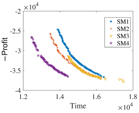
Figure 7. The pareto front corresponding to the median HV values obtained by MOFECO-MS algorithm with four search methods.

The results in Figure 7 are also consistent with those in Table 13. Since the objective function of this paper is to minimize, the closer the frontier curve is to the lower left, the better the algorithm effect will be. From Figure 7, the accuracy and distribution of each search method can also be seen intuitively, and SM4 is obviously better than the other three methods.

5.3. Experimental Results and Discussion on Algorithms Comparison

To evaluate the performance of our proposed MOFECO-MS algorithm, we compare it with eight other intelligent optimization algorithms based on different mechanisms. These include the classic Non-Dominated Sorting Genetic Algorithm II (NSGAII) [26], the Multi-objective Particle Swarm Optimization (MOPSO) [33], the Multi-Objective Whale Optimization Algorithm (MOWOA) [34], the Multi-objective Grey Wolf Optimization (MOGWO) [35], the Multi-objective Aquila Optimizer (MOAO) [36], and the Multi-Objective Honey Badger algorithm (MOHBA) [37], all proposed in recent years. Additionally, we include the basic Multi-Objective Five-element Cycle Optimization algorithm (MOFECO) [24] and a Local Search Many-Objective Five-element Cycle optimization algorithm (LSMOFECO) [25].

MOWOA mimics humpback whale hunting behavior, while MOGWO simulates gray wolf group predation behavior. MOAO and MOHBA, proposed in the last two years, are inspired by eagles’ hunting and honey badgers’ foraging behavior, respectively. The parameters for MOWOA, MOGWO, MOAO, and MOHBA remain consistent with their original literature. NSGAII employs the same crossover and mutation operators as MOFECO-MS, with crossover and mutation probabilities set to $0.9$ and $0.1$, respectively. MOFECO and LSMOFECO utilize parameters identical to those in MOFECO-MS. All eight algorithms share a population size of $N=100$. The termination criterion for each algorithm is when the number of objective function evaluations reaches 100,000 ($c_{\max }=N\times 1000$).

We conduct 15 independent runs for each algorithm on the BITTP instances in Table 5. The experimental results are presented in Table 14, Table 15, Table 16, Table 17, Table 18, Table 19, Table 20, Table 21, Table 22, Table 23, Table 24, Table 25, Table 26, Table 27, Table 28, Table 29, Table 30, Table 31, Table 32, Table 33, Table 34, Table 35, Table 36, Table 37, Table 38, Table 39 and Table 40, Figure 8, Figure 9, Figure 10, Figure 11, Figure 12, Figure 13, Figure 14, Figure 15 and Figure 16.

Table 14. Statistical results of HV indicator of the eight comparison algorithms for $eil51\text{\_}n50$.

	Best	Worst	Median	Average	StdDev
NSGAII	1.32 × ${10}^9$	6.15 × ${10}^8$	8.28 × ${10}^8$	8.64 × ${10}^8$	2.18 × ${10}^8$
MOPSO	8.55 × ${10}^8$	3.35 × ${10}^8$	5.47 × ${10}^8$	5.50 × ${10}^8$	1.39 × ${10}^8$
MOAO	2.65 × ${10}^9$	3.97 × ${10}^8$	6.69 × ${10}^8$	9.46 × ${10}^8$	7.26 × ${10}^8$
MOHBA	6.99 × ${10}^8$	2.80 × ${10}^8$	4.69 × ${10}^8$	4.58 × ${10}^8$	1.24 × ${10}^8$
MOWOA	7.01 × ${10}^8$	3.42 × ${10}^8$	4.56 × ${10}^8$	4.65 × ${10}^8$	1.02 × ${10}^8$
MOGWO	7.26 × ${10}^8$	2.04 × ${10}^8$	4.48 × ${10}^8$	4.61 × ${10}^8$	1.29 × ${10}^8$
MOFECO	1.25 × ${10}^9$	4.29 × ${10}^8$	7.67 × ${10}^8$	7.34 × ${10}^8$	2.58 × ${10}^8$
LSMOFECO	2.32 × ${10}^9$	7.20 × ${10}^8$	1.65 × ${10}^9$	1.54 × ${10}^9$	4.84 × ${10}^8$
MOFECO-MS	3.35 × ${10}^9$	1.15 × ${10}^9$	2.22 × ${10}^9$	2.30 × ${10}^9$	5.73 × ${10}^8$

Table 15. Statistical results of SP indicator of the eight comparison algorithms for $eil{51}_{\text{\_}}n50$.

	Best	Worst	Median	Average	StdDev
NSGAII	4.68 × ${10}^1$	2.40 × ${10}^2$	9.30 × ${10}^1$	1.17 × ${10}^2$	6.46 × ${10}^1$
MOPSO	1.06 × ${10}^2$	8.36 × ${10}^2$	3.22 × ${10}^2$	3.85 × ${10}^2$	2.13 × ${10}^2$
MOAO	9.73 × ${10}^1$	6.38 × ${10}^2$	2.94 × ${10}^2$	3.31 × ${10}^2$	1.71 × ${10}^2$
MOHBA	1.84 × ${10}^2$	7.65 × ${10}^2$	3.31 × ${10}^2$	3.41 × ${10}^2$	1.36 × ${10}^2$
MOWOA	1.29 × ${10}^2$	1.21 × ${10}^3$	4.19 × ${10}^2$	4.87 × ${10}^2$	3.19 × ${10}^2$
MOGWO	8.52 × ${10}^1$	1.01 × ${10}^3$	4.06 × ${10}^2$	4.51 × ${10}^2$	3.02 × ${10}^2$
MOFECO	7.89 × ${10}^1$	4.89 × ${10}^2$	1.59 × ${10}^2$	1.86 × ${10}^2$	1.11 × ${10}^2$
LSMOFECO	2.19 × ${10}^1$	7.16 × ${10}^1$	3.83 × ${10}^1$	4.04 × ${10}^1$	1.37 × ${10}^1$
MOFECO-MS	2.57 × ${10}^1$	8.12 × ${10}^1$	3.91 × ${10}^1$	4.26 × ${10}^1$	1.58 × ${10}^1$

Table 16. Statistical results of PD indicator of the eight comparison algorithms for $eil{51}_{\text{\_}}n50$.

	Best	Worst	Median	Average	StdDev
NSGAII	1.57 × ${10}^6$	3.65 × ${10}^5$	7.03 × ${10}^5$	7.50 × ${10}^5$	2.70 × ${10}^5$
MOPSO	4.57 × ${10}^6$	2.03 × ${10}^6$	3.30 × ${10}^6$	3.21 × ${10}^6$	7.51 × ${10}^5$
MOAO	3.48 × ${10}^6$	1.72 × ${10}^6$	2.58 × ${10}^6$	2.70 × ${10}^6$	4.64 × ${10}^5$
MOHBA	4.13 × ${10}^6$	1.78 × ${10}^6$	2.89 × ${10}^6$	2.86 × ${10}^6$	5.57 × ${10}^5$
MOWOA	3.76 × ${10}^6$	2.00 × ${10}^6$	2.84 × ${10}^6$	2.81 × ${10}^6$	5.81 × ${10}^5$
MOGWO	4.16 × ${10}^6$	2.12 × ${10}^6$	2.77 × ${10}^6$	2.95 × ${10}^6$	6.04 × ${10}^5$
MOFECO	3.91 × ${10}^6$	1.47 × ${10}^6$	2.06 × ${10}^6$	2.12 × ${10}^6$	6.09 × ${10}^5$
LSMOFECO	1.70 × ${10}^6$	6.19 × ${10}^5$	1.01 × ${10}^6$	1.03 × ${10}^6$	3.36 × ${10}^5$
MOFECO-MS	2.24 × ${10}^6$	7.43 × ${10}^5$	1.38 × ${10}^6$	1.42 × ${10}^6$	4.10 × ${10}^5$

Table 17. Statistical results of HV indicator of the eight comparison algorithms for $eil51\text{\_}n250$.

	Best	Worst	Median	Average	StdDev
NSGAII	5.94 × ${10}^9$	2.51 × ${10}^9$	3.83 × ${10}^9$	3.93 × ${10}^9$	1.02 × ${10}^9$
MOPSO	7.53 × ${10}^8$	2.88 × ${10}^8$	5.92 × ${10}^8$	5.69 × ${10}^8$	1.38 × ${10}^8$
MOAO	9.97 × ${10}^8$	3.06 × ${10}^8$	5.12 × ${10}^8$	5.34 × ${10}^8$	1.68 × ${10}^8$
MOHBA	7.41 × ${10}^8$	1.70 × ${10}^8$	4.48 × ${10}^8$	4.42 × ${10}^8$	1.37 × ${10}^8$
MOWOA	7.92 × ${10}^8$	2.31 × ${10}^8$	4.35 × ${10}^8$	4.79 × ${10}^8$	1.59 × ${10}^8$
MOGWO	6.99 × ${10}^8$	1.59 × ${10}^8$	4.39 × ${10}^8$	4.28 × ${10}^8$	1.37 × ${10}^8$
MOFECO	5.04 × ${10}^9$	2.00 × ${10}^9$	3.57 × ${10}^9$	3.48 × ${10}^9$	7.97 × ${10}^8$
LSMOFECO	9.46 × ${10}^9$	4.56 × ${10}^9$	9.00 × ${10}^9$	8.47 × ${10}^9$	1.30 × ${10}^9$
MOFECO-MS	9.57 × ${10}^9$	7.71 × ${10}^9$	8.64 × ${10}^9$	8.76 × ${10}^9$	4.70 × ${10}^8$

Table 18. Statistical results of SP indicator of the eight comparison algorithms for $eil{51}_{\text{\_}}n250$.

	Best	Worst	Median	Average	StdDev
NSGAII	4.70 × ${10}^1$	2.29 × ${10}^2$	1.34 × ${10}^2$	1.40 × ${10}^2$	5.71 × ${10}^1$
MOPSO	2.11 × ${10}^2$	8.59 × ${10}^2$	3.80 × ${10}^2$	4.67 × ${10}^2$	2.23 × ${10}^2$
MOAO	2.10 × ${10}^2$	6.60 × ${10}^2$	3.99 × ${10}^2$	4.25 × ${10}^2$	1.33 × ${10}^2$
MOHBA	1.67 × ${10}^2$	1.21 × ${10}^3$	4.10 × ${10}^2$	5.20 × ${10}^2$	2.91 × ${10}^2$
MOWOA	2.84 × ${10}^2$	1.38 × ${10}^3$	5.10 × ${10}^2$	5.66 × ${10}^2$	2.79 × ${10}^2$
MOGWO	1.86 × ${10}^2$	1.43 × ${10}^3$	5.07 × ${10}^2$	5.63 × ${10}^2$	3.57 × ${10}^2$
MOFECO	8.55 × ${10}^1$	4.89 × ${10}^2$	1.65 × ${10}^2$	1.89 × ${10}^2$	1.09 × ${10}^2$
LSMOFECO	6.91 × ${10}^1$	1.91 × ${10}^2$	7.76 × ${10}^1$	8.51 × ${10}^1$	2.99 × ${10}^1$
MOFECO-MS	3.45 × ${10}^1$	1.81 × ${10}^2$	6.11 × ${10}^1$	6.65 × ${10}^1$	3.52 × ${10}^1$

Table 19. Statistical results of PD indicator of the eight comparison algorithms for $eil{51}_{\text{\_}}n250$.

	Best	Worst	Median	Average	StdDev
NSGAII	3.23 × ${10}^6$	1.46 × ${10}^6$	1.92 × ${10}^6$	2.00 × ${10}^6$	4.55 × ${10}^5$
MOPSO	3.78 × ${10}^6$	2.22 × ${10}^6$	2.75 × ${10}^6$	2.82 × ${10}^6$	4.71 × ${10}^5$
MOAO	4.01 × ${10}^6$	1.69 × ${10}^6$	2.80 × ${10}^6$	2.72 × ${10}^6$	7.15 × ${10}^5$
MOHBA	3.34 × ${10}^6$	1.75 × ${10}^6$	2.58 × ${10}^6$	2.49 × ${10}^6$	5.21 × ${10}^5$
MOWOA	4.61 × ${10}^6$	1.55 × ${10}^6$	2.84 × ${10}^6$	2.87 × ${10}^6$	7.61 × ${10}^5$
MOGWO	3.66 × ${10}^6$	1.58 × ${10}^6$	2.58 × ${10}^6$	2.57 × ${10}^6$	6.35 × ${10}^5$
MOFECO	6.84 × ${10}^6$	4.11 × ${10}^6$	5.20 × ${10}^6$	5.34 × ${10}^6$	8.68 × ${10}^5$
LSMOFECO	3.73 × ${10}^6$	1.67 × ${10}^6$	2.69 × ${10}^6$	2.59 × ${10}^6$	6.38 × ${10}^5$
MOFECO-MS	4.19 × ${10}^6$	1.89 × ${10}^6$	2.95 × ${10}^6$	3.02 × ${10}^6$	5.31 × ${10}^5$

Table 20. Statistical results of HV indicator of the eight comparison algorithms for $eil51\text{\_}n500$.

	Best	Worst	Median	Average	StdDev
NSGAII	1.84 × ${10}^{10}$	8.05 × ${10}^9$	1.10 × ${10}^{10}$	1.16 × ${10}^{10}$	2.88 × ${10}^9$
MOPSO	1.26 × ${10}^9$	4.33 × ${10}^8$	8.43 × ${10}^8$	8.80 × ${10}^8$	2.31 × ${10}^8$
MOAO	1.20 × ${10}^9$	5.77 × ${10}^8$	9.32 × ${10}^8$	8.86 × ${10}^8$	1.81 × ${10}^8$
MOHBA	3.46 × ${10}^8$	1.02 × ${10}^8$	2.37 × ${10}^8$	2.24 × ${10}^8$	7.30 × ${10}^7$
MOWOA	1.03 × ${10}^9$	3.67 × ${10}^8$	6.94 × ${10}^8$	7.32 × ${10}^8$	1.76 × ${10}^8$
MOGWO	9.00 × ${10}^8$	4.39 × ${10}^8$	7.48 × ${10}^8$	7.19 × ${10}^8$	1.36 × ${10}^8$
MOFECO	1.42 × ${10}^{10}$	6.98 × ${10}^9$	1.09 × ${10}^{10}$	1.05 × ${10}^{10}$	1.83 × ${10}^9$
LSMOFECO	3.84 × ${10}^{10}$	1.96 × ${10}^{10}$	3.75 × ${10}^{10}$	3.43 × ${10}^{10}$	6.37 × ${10}^9$
MOFECO-MS	3.90 × ${10}^{10}$	2.60 × ${10}^{10}$	3.78 × ${10}^{10}$	3.70 × ${10}^{10}$	3.10 × ${10}^9$

Table 21. Statistical results of SP indicator of the eight comparison algorithms for $eil{51}_{\text{\_}}n500$.

	Best	Worst	Median	Average	StdDev
NSGAII	9.95 × ${10}^1$	5.64 × ${10}^2$	3.03 × ${10}^2$	2.99 × ${10}^2$	1.38 × ${10}^2$
MOPSO	3.87 × ${10}^2$	1.72 × ${10}^3$	6.71 × ${10}^2$	7.76 × ${10}^2$	3.44 × ${10}^2$
MOAO	2.85 × ${10}^2$	1.77 × ${10}^3$	5.53 × ${10}^2$	7.72 × ${10}^2$	4.57 × ${10}^2$
MOHBA	2.26 × ${10}^2$	7.95 × ${10}^2$	4.24 × ${10}^2$	4.75 × ${10}^2$	1.89 × ${10}^2$
MOWOA	5.53 × ${10}^2$	2.44 × ${10}^3$	1.06 × ${10}^3$	1.09 × ${10}^3$	5.25 × ${10}^2$
MOGWO	2.69 × ${10}^2$	1.76 × ${10}^3$	8.95 × ${10}^2$	9.98 × ${10}^2$	4.32 × ${10}^2$
MOFECO	1.36 × ${10}^2$	8.22 × ${10}^2$	3.28 × ${10}^2$	3.84 × ${10}^2$	2.08 × ${10}^2$
LSMOFECO	2.82 × ${10}^1$	1.03 × ${10}^2$	5.85 × ${10}^1$	6.36 × ${10}^1$	2.48 × ${10}^1$
MOFECO-MS	3.42 × ${10}^1$	1.11 × ${10}^2$	5.38 × ${10}^1$	5.77 × ${10}^1$	1.99 × ${10}^1$

Table 22. Statistical results of PD indicator of the eight comparison algorithms for $eil{51}_{\text{\_}}n500$.

	Best	Worst	Median	Average	StdDev
NSGAII	4.32 × ${10}^6$	1.67 × ${10}^6$	2.51 × ${10}^6$	2.62 × ${10}^6$	7.17 × ${10}^5$
MOPSO	6.00 × ${10}^6$	3.27 × ${10}^6$	4.46 × ${10}^6$	4.37 × ${10}^6$	8.59 × ${10}^5$
MOAO	7.95 × ${10}^6$	2.57 × ${10}^6$	5.00 × ${10}^6$	4.84 × ${10}^6$	1.24 × ${10}^6$
MOHBA	4.00 × ${10}^6$	1.59 × ${10}^6$	2.66 × ${10}^6$	2.77 × ${10}^6$	6.98 × ${10}^5$
MOWOA	7.60 × ${10}^6$	2.97 × ${10}^6$	4.20 × ${10}^6$	4.58 × ${10}^6$	1.22 × ${10}^6$
MOGWO	6.53 × ${10}^6$	2.31 × ${10}^6$	4.28 × ${10}^6$	4.32 × ${10}^6$	1.31 × ${10}^6$
MOFECO	1.01 × ${10}^7$	5.57 × ${10}^6$	8.54 × ${10}^6$	8.11 × ${10}^6$	1.15 × ${10}^6$
LSMOFECO	3.64 × ${10}^6$	1.44 × ${10}^6$	2.45 × ${10}^6$	2.64 × ${10}^6$	6.51 × ${10}^5$
MOFECO-MS	4.91 × ${10}^6$	2.31 × ${10}^6$	3.27 × ${10}^6$	3.37 × ${10}^6$	7.97 × ${10}^5$

Table 23. Statistical results of HV indicator of the eight comparison algorithms for $ch150\text{\_}n149$.

	Best	Worst	Median	Average	StdDev
NSGAII	1.04 × ${10}^{11}$	4.49 × ${10}^{10}$	6.91 × ${10}^{10}$	7.09 × ${10}^{10}$	1.62 × ${10}^{10}$
MOPSO	2.17 × ${10}^{10}$	9.26 × ${10}^9$	1.44 × ${10}^{10}$	1.45 × ${10}^{10}$	3.58 × ${10}^9$
MOAO	2.43 × ${10}^{10}$	1.06 × ${10}^{10}$	1.74 × ${10}^{10}$	1.74 × ${10}^{10}$	4.30 × ${10}^9$
MOHBA	2.03 × ${10}^{10}$	1.07 × ${10}^{10}$	1.63 × ${10}^{10}$	1.59 × ${10}^{10}$	3.07 × ${10}^9$
MOWOA	1.90 × ${10}^{10}$	9.07 × ${10}^9$	1.27 × ${10}^{10}$	1.32 × ${10}^{10}$	2.64 × ${10}^9$
MOGWO	1.68 × ${10}^{10}$	7.24 × ${10}^9$	1.24 × ${10}^{10}$	1.27 × ${10}^{10}$	2.76 × ${10}^9$
MOFECO	8.29 × ${10}^{10}$	2.44 × ${10}^{10}$	3.86 × ${10}^{10}$	4.27 × ${10}^{10}$	1.57 × ${10}^{10}$
LSMOFECO	1.80 × ${10}^{11}$	4.62 × ${10}^{10}$	1.00 × ${10}^{11}$	1.09 × ${10}^{11}$	3.39 × ${10}^{10}$
MOFECO-MS	1.87 × ${10}^{11}$	7.27 × ${10}^{10}$	1.37 × ${10}^{11}$	1.34 × ${10}^{11}$	3.35 × ${10}^{10}$

Table 24. Statistical results of SP indicator of the eight comparison algorithms for $ch150\text{\_}n149$.

	Best	Worst	Median	Average	StdDev
NSGAII	3.68 × ${10}^2$	6.44 × ${10}^3$	9.33 × ${10}^2$	1.33 × ${10}^3$	1.50 × ${10}^3$
MOPSO	1.03 × ${10}^3$	1.45 × ${10}^4$	5.18 × ${10}^3$	5.81 × ${10}^3$	3.52 × ${10}^3$
MOAO	1.30 × ${10}^3$	2.04 × ${10}^4$	2.87 × ${10}^3$	5.48 × ${10}^3$	5.57 × ${10}^3$
MOHBA	1.46 × ${10}^3$	4.42 × ${10}^4$	6.68 × ${10}^3$	1.03 × ${10}^4$	1.10 × ${10}^4$
MOWOA	1.63 × ${10}^3$	1.30 × ${10}^4$	4.51 × ${10}^3$	5.21 × ${10}^3$	2.93 × ${10}^3$
MOGWO	1.45 × ${10}^3$	1.47 × ${10}^4$	4.85 × ${10}^3$	6.10 × ${10}^3$	3.85 × ${10}^3$
MOFECO	2.30 × ${10}^2$	1.14 × ${10}^4$	4.66 × ${10}^2$	1.31 × ${10}^3$	2.82 × ${10}^3$
LSMOFECO	1.38 × ${10}^2$	1.00 × ${10}^3$	2.01 × ${10}^2$	2.99 × ${10}^2$	2.27 × ${10}^2$
MOFECO-MS	2.51 × ${10}^1$	2.79 × ${10}^2$	8.08 × ${10}^1$	1.10 × ${10}^2$	6.69 × ${10}^1$

Table 25. Statistical results of PD indicator of the eight comparison algorithms for $ch150\text{\_}n149$.

	Best	Worst	Median	Average	StdDev
NSGAII	2.02 × ${10}^7$	3.59 × ${10}^6$	1.19 × ${10}^7$	1.22 × ${10}^7$	3.67 × ${10}^6$
MOPSO	2.28 × ${10}^7$	1.24 × ${10}^7$	2.12 × ${10}^7$	1.99 × ${10}^7$	2.90 × ${10}^6$
MOAO	3.89 × ${10}^7$	1.57 × ${10}^7$	2.19 × ${10}^7$	2.28 × ${10}^7$	5.62 × ${10}^6$
MOHBA	2.95 × ${10}^7$	1.50 × ${10}^7$	2.02 × ${10}^7$	2.10 × ${10}^7$	4.46 × ${10}^6$
MOWOA	2.84 × ${10}^7$	1.05 × ${10}^7$	2.29 × ${10}^7$	2.16 × ${10}^7$	4.80 × ${10}^6$
MOGWO	2.80 × ${10}^7$	1.30 × ${10}^7$	1.83 × ${10}^7$	1.95 × ${10}^7$	4.64 × ${10}^6$
MOFECO	2.95 × ${10}^7$	1.66 × ${10}^7$	2.09 × ${10}^7$	2.22 × ${10}^7$	4.00 × ${10}^6$
LSMOFECO	1.53 × ${10}^7$	4.00 × ${10}^6$	9.63 × ${10}^6$	1.00 × ${10}^7$	2.80 × ${10}^6$
MOFECO-MS	1.18 × ${10}^7$	3.92 × ${10}^6$	8.56 × ${10}^6$	8.40 × ${10}^6$	2.26 × ${10}^6$

Table 26. Statistical results of HV indicator of the eight comparison algorithms for $ch150\text{\_}n745$.

	Best	Worst	Median	Average	StdDev
NSGAII	2.56 × ${10}^{11}$	1.45 × ${10}^{11}$	2.05 × ${10}^{11}$	2.05 × ${10}^{11}$	3.42 × ${10}^{10}$
MOPSO	1.63 × ${10}^{10}$	5.72 × ${10}^9$	9.31 × ${10}^9$	9.10 × ${10}^9$	2.83 × ${10}^9$
MOAO	1.56 × ${10}^{10}$	6.53 × ${10}^9$	1.09 × ${10}^{10}$	1.02 × ${10}^{10}$	2.43 × ${10}^9$
MOHBA	1.56 × ${10}^{10}$	4.86 × ${10}^9$	9.17 × ${10}^9$	9.49 × ${10}^9$	3.04 × ${10}^9$
MOWOA	1.07 × ${10}^{10}$	4.35 × ${10}^9$	6.58 × ${10}^9$	7.10 × ${10}^9$	1.79 × ${10}^9$
MOGWO	9.90 × ${10}^9$	3.49 × ${10}^9$	7.49 × ${10}^9$	7.44 × ${10}^9$	1.78 × ${10}^9$
MOFECO	2.05 × ${10}^{11}$	9.50 × ${10}^{10}$	1.66 × ${10}^{11}$	1.59 × ${10}^{11}$	2.77 × ${10}^{10}$
LSMOFECO	6.60 × ${10}^{10}$	2.58 × ${10}^{10}$	4.90 × ${10}^{10}$	4.53 × ${10}^{10}$	1.45 × ${10}^{10}$
MOFECO-MS	4.66 × ${10}^{11}$	2.37 × ${10}^{11}$	4.07 × ${10}^{11}$	3.63 × ${10}^{11}$	8.70 × ${10}^{10}$

Table 27. Statistical results of SP indicator of the eight comparison algorithms for $ch150\text{\_}n745$.

	Best	Worst	Median	Average	StdDev
NSGAII	2.15 × ${10}^2$	6.19 × ${10}^3$	6.86 × ${10}^2$	1.51 × ${10}^3$	1.85 × ${10}^3$
MOPSO	1.39 × ${10}^3$	7.35 × ${10}^3$	2.76 × ${10}^3$	3.22 × ${10}^3$	1.83 × ${10}^3$
MOAO	1.22 × ${10}^3$	1.06 × ${10}^4$	2.93 × ${10}^3$	3.78 × ${10}^3$	2.47 × ${10}^3$
MOHBA	6.23 × ${10}^2$	1.17 × ${10}^4$	2.99 × ${10}^3$	4.38 × ${10}^3$	3.71 × ${10}^3$
MOWOA	1.39 × ${10}^3$	9.61 × ${10}^3$	3.94 × ${10}^3$	4.54 × ${10}^3$	2.63 × ${10}^3$
MOGWO	1.75 × ${10}^3$	9.40 × ${10}^3$	2.96 × ${10}^3$	3.80 × ${10}^3$	2.10 × ${10}^3$
MOFECO	1.62 × ${10}^2$	3.90 × ${10}^2$	3.15 × ${10}^2$	2.90 × ${10}^2$	5.98 × ${10}^1$
LSMOFECO	9.59 × ${10}^1$	2.76 × ${10}^2$	1.71 × ${10}^2$	1.89 × ${10}^2$	5.92 × ${10}^1$
MOFECO-MS	4.91 × ${10}^1$	2.11 × ${10}^2$	1.11 × ${10}^2$	1.20 × ${10}^2$	4.68 × ${10}^1$

Table 28. Statistical results of PD indicator of the eight comparison algorithms for $ch150\text{\_}n745$.

	Best	Worst	Median	Average	StdDev
NSGAII	2.29 × ${10}^7$	1.17 × ${10}^7$	1.70 × ${10}^7$	1.70 × ${10}^7$	3.06 × ${10}^6$
MOPSO	2.51 × ${10}^7$	1.08 × ${10}^7$	1.83 × ${10}^7$	1.81 × ${10}^7$	4.42 × ${10}^6$
MOAO	2.59 × ${10}^7$	1.48 × ${10}^7$	1.82 × ${10}^7$	1.91 × ${10}^7$	3.44 × ${10}^6$
MOHBA	3.09 × ${10}^7$	1.06 × ${10}^7$	2.03 × ${10}^7$	1.95 × ${10}^7$	5.22 × ${10}^6$
MOWOA	2.24 × ${10}^7$	1.41 × ${10}^7$	1.70 × ${10}^7$	1.72 × ${10}^7$	2.37 × ${10}^6$
MOGWO	3.23 × ${10}^7$	1.19 × ${10}^7$	1.79 × ${10}^7$	1.92 × ${10}^7$	6.13 × ${10}^6$
MOFECO	7.34 × ${10}^7$	3.39 × ${10}^7$	4.73 × ${10}^7$	4.88 × ${10}^7$	9.50 × ${10}^6$
LSMOFECO	1.24 × ${10}^7$	7.59 × ${10}^6$	9.84 × ${10}^6$	1.00 × ${10}^7$	1.49 × ${10}^6$
MOFECO-MS	1.25 × ${10}^7$	5.86 × ${10}^6$	8.66 × ${10}^6$	8.67 × ${10}^6$	1.95 × ${10}^6$

Table 29. Statistical results of HV indicator of the eight comparison algorithms for $ch150\text{\_}n1490$.

	Best	Worst	Median	Average	StdDev
NSGAII	1.19 × ${10}^{12}$	6.03 × ${10}^{11}$	9.48 × ${10}^{11}$	9.07 × ${10}^{11}$	1.77 × ${10}^{11}$
MOPSO	2.49 × ${10}^{10}$	9.45 × ${10}^9$	1.90 × ${10}^{10}$	1.83 × ${10}^{10}$	3.98 × ${10}^9$
MOAO	2.95 × ${10}^{10}$	1.06 × ${10}^{10}$	1.84 × ${10}^{10}$	1.87 × ${10}^{10}$	5.92 × ${10}^9$
MOHBA	3.33 × ${10}^{10}$	1.22 × ${10}^{10}$	1.98 × ${10}^{10}$	1.96 × ${10}^{10}$	5.54 × ${10}^9$
MOWOA	2.78 × ${10}^{10}$	1.04 × ${10}^{10}$	1.74 × ${10}^{10}$	1.80 × ${10}^{10}$	4.47 × ${10}^9$
MOGWO	2.05 × ${10}^{10}$	6.33 × ${10}^9$	1.49 × ${10}^{10}$	1.46 × ${10}^{10}$	4.12 × ${10}^9$
MOFECO	7.62 × ${10}^{11}$	5.30 × ${10}^{11}$	6.15 × ${10}^{11}$	6.21 × ${10}^{11}$	6.68 × ${10}^{10}$
LSMOFECO	1.49 × ${10}^{12}$	5.19 × ${10}^{11}$	1.04 × ${10}^{12}$	9.92 × ${10}^{11}$	2.78 × ${10}^{11}$
MOFECO-MS	2.84 × ${10}^{12}$	9.04 × ${10}^{11}$	2.36 × ${10}^{12}$	2.18 × ${10}^{12}$	6.50 × ${10}^{11}$

Table 30. Statistical results of SP indicator of the eight comparison algorithms for $ch150\text{\_}n1490$.

	Best	Worst	Median	Average	StdDev
NSGAII	3.22 × ${10}^2$	4.22 × ${10}^3$	1.16 × ${10}^3$	1.44 × ${10}^3$	9.39 × ${10}^2$
MOPSO	1.94 × ${10}^3$	6.53 × ${10}^3$	2.84 × ${10}^3$	3.48 × ${10}^3$	1.53 × ${10}^3$
MOAO	1.35 × ${10}^3$	1.71 × ${10}^4$	3.22 × ${10}^3$	4.43 × ${10}^3$	3.92 × ${10}^3$
MOHBA	1.40 × ${10}^3$	1.25 × ${10}^4$	2.71 × ${10}^3$	4.12 × ${10}^3$	3.18 × ${10}^3$
MOWOA	1.46 × ${10}^3$	1.55 × ${10}^4$	2.78 × ${10}^3$	3.86 × ${10}^3$	3.51 × ${10}^3$
MOGWO	2.22 × ${10}^3$	6.41 × ${10}^3$	3.93 × ${10}^3$	4.01 × ${10}^3$	1.42 × ${10}^3$
MOFECO	1.94 × ${10}^2$	1.58 × ${10}^3$	3.85 × ${10}^2$	5.24 × ${10}^2$	3.76 × ${10}^2$
LSMOFECO	1.87 × ${10}^2$	3.49 × ${10}^3$	3.05 × ${10}^2$	5.99 × ${10}^2$	8.25 × ${10}^2$
MOFECO-MS	6.66 × ${10}^1$	7.83 × ${10}^2$	1.50 × ${10}^2$	2.11 × ${10}^2$	1.79 × ${10}^2$

Table 31. Statistical results of PD indicator of the eight comparison algorithms for $ch150\text{\_}n1490$.

	Best	Worst	Median	Average	StdDev
NSGAII	3.58 × ${10}^7$	1.40 × ${10}^7$	2.28 × ${10}^7$	2.37 × ${10}^7$	5.88 × ${10}^6$
MOPSO	3.88 × ${10}^7$	2.00 × ${10}^7$	2.95 × ${10}^7$	2.90 × ${10}^7$	5.98 × ${10}^6$
MOAO	3.67 × ${10}^7$	1.97 × ${10}^7$	2.41 × ${10}^7$	2.53 × ${10}^7$	5.00 × ${10}^6$
MOHBA	3.64 × ${10}^7$	1.67 × ${10}^7$	2.43 × ${10}^7$	2.52 × ${10}^7$	5.59 × ${10}^6$
MOWOA	3.61 × ${10}^7$	1.92 × ${10}^7$	2.74 × ${10}^7$	2.69 × ${10}^7$	4.63 × ${10}^6$
MOGWO	3.48 × ${10}^7$	1.46 × ${10}^7$	2.64 × ${10}^7$	2.55 × ${10}^7$	6.42 × ${10}^6$
MOFECO	8.63 × ${10}^7$	4.86 × ${10}^7$	5.86 × ${10}^7$	6.04 × ${10}^7$	1.06 × ${10}^7$
LSMOFECO	1.43 × ${10}^7$	4.64 × ${10}^6$	9.36 × ${10}^6$	9.46 × ${10}^6$	2.56 × ${10}^6$
MOFECO-MS	1.67 × ${10}^7$	6.56 × ${10}^6$	9.08 × ${10}^6$	9.65 × ${10}^6$	2.53 × ${10}^6$

Table 32. Statistical results of HV indicator of the eight comparison algorithms for $a280\text{\_}n279$.

	Best	Worst	Median	Average	StdDev
NSGAII	2.62 × ${10}^{11}$	1.43 × ${10}^{11}$	2.43 × ${10}^{11}$	2.34 × ${10}^{11}$	3.71 × ${10}^{10}$
MOPSO	3.23 × ${10}^{10}$	1.81 × ${10}^{10}$	2.24 × ${10}^{10}$	2.41 × ${10}^{10}$	4.27 × ${10}^9$
MOAO	3.48 × ${10}^{10}$	1.75 × ${10}^{10}$	2.55 × ${10}^{10}$	2.60 × ${10}^{10}$	4.56 × ${10}^9$
MOHBA	3.78 × ${10}^{10}$	1.67 × ${10}^{10}$	3.00 × ${10}^{10}$	2.94 × ${10}^{10}$	5.72 × ${10}^9$
MOWOA	4.76 × ${10}^{10}$	1.94 × ${10}^{10}$	3.42 × ${10}^{10}$	3.45 × ${10}^{10}$	7.74 × ${10}^9$
MOGWO	4.17 × ${10}^{10}$	2.00 × ${10}^{10}$	2.55 × ${10}^{10}$	2.78 × ${10}^{10}$	6.42 × ${10}^9$
MOFECO	2.00 × ${10}^{10}$	1.20 × ${10}^{10}$	1.64 × ${10}^{10}$	1.63 × ${10}^{10}$	2.28 × ${10}^9$
LSMOFECO	2.79 × ${10}^{11}$	1.05 × ${10}^{11}$	1.86 × ${10}^{11}$	1.89 × ${10}^{11}$	5.10 × ${10}^{10}$
MOFECO-MS	3.25 × ${10}^{11}$	2.79 × ${10}^{11}$	2.93 × ${10}^{11}$	2.98 × ${10}^{11}$	1.25 × ${10}^{10}$

Table 33. Statistical results of SP indicator of the eight comparison algorithms for $a280\text{\_}n279$.

	Best	Worst	Median	Average	StdDev
NSGAII	6.39 × ${10}^1$	7.36 × ${10}^2$	1.81 × ${10}^2$	2.42 × ${10}^2$	1.82 × ${10}^2$
MOPSO	1.01 × ${10}^3$	8.85 × ${10}^3$	2.95 × ${10}^3$	3.37 × ${10}^3$	2.04 × ${10}^3$
MOAO	1.16 × ${10}^3$	7.31 × ${10}^3$	2.55 × ${10}^3$	2.92 × ${10}^3$	1.76 × ${10}^3$
MOHBA	8.93 × ${10}^2$	6.70 × ${10}^3$	2.57 × ${10}^3$	2.82 × ${10}^3$	1.65 × ${10}^3$
MOWOA	7.34 × ${10}^2$	3.43 × ${10}^3$	1.44 × ${10}^3$	1.60 × ${10}^3$	7.71 × ${10}^2$
MOGWO	6.67 × ${10}^2$	5.28 × ${10}^3$	1.66 × ${10}^3$	2.31 × ${10}^3$	1.67 × ${10}^3$
MOFECO	2.03 × ${10}^2$	1.18 × ${10}^3$	3.24 × ${10}^2$	3.77 × ${10}^2$	2.36 × ${10}^2$
LSMOFECO	7.86 × ${10}^1$	2.52 × ${10}^2$	1.36 × ${10}^2$	1.43 × ${10}^2$	5.61 × ${10}^1$
MOFECO-MS	3.40 × ${10}^1$	1.07 × ${10}^2$	6.69 × ${10}^1$	7.10 × ${10}^1$	2.07 × ${10}^1$

Table 34. Statistical results of PD indicator of the eight comparison algorithms for $a280\text{\_}n279$.

	Best	Worst	Median	Average	StdDev
NSGAII	1.93 × ${10}^7$	3.83 × ${10}^6$	9.63 × ${10}^6$	9.92 × ${10}^6$	3.44 × ${10}^6$
MOPSO	1.87 × ${10}^7$	1.02 × ${10}^7$	1.44 × ${10}^7$	1.42 × ${10}^7$	2.52 × ${10}^6$
MOAO	2.40 × ${10}^7$	1.03 × ${10}^7$	1.66 × ${10}^7$	1.75 × ${10}^7$	3.47 × ${10}^6$
MOHBA	2.76 × ${10}^7$	8.48 × ${10}^6$	1.49 × ${10}^7$	1.55 × ${10}^7$	4.51 × ${10}^6$
MOWOA	2.05 × ${10}^7$	1.23 × ${10}^7$	1.48 × ${10}^7$	1.58 × ${10}^7$	2.45 × ${10}^6$
MOGWO	2.19 × ${10}^7$	1.16 × ${10}^7$	1.73 × ${10}^7$	1.71 × ${10}^7$	2.68 × ${10}^6$
MOFECO	3.94 × ${10}^7$	1.57 × ${10}^7$	2.63 × ${10}^7$	2.59 × ${10}^7$	7.38 × ${10}^6$
LSMOFECO	1.40 × ${10}^7$	4.26 × ${10}^6$	6.84 × ${10}^6$	7.59 × ${10}^6$	2.73 × ${10}^6$
MOFECO-MS	1.06 × ${10}^7$	4.61 × ${10}^6$	5.97 × ${10}^6$	6.25 × ${10}^6$	1.47 × ${10}^6$

Table 35. Statistical results of HV indicator of the eight comparison algorithms for $a280\text{\_}n1395$.

	Best	Worst	Median	Average	StdDev
NSGAII	5.48 × ${10}^{11}$	2.53 × ${10}^{11}$	4.70 × ${10}^{11}$	4.44 × ${10}^{11}$	8.99 × ${10}^{10}$
MOPSO	3.06 × ${10}^{10}$	5.02 × ${10}^9$	1.76 × ${10}^{10}$	1.80 × ${10}^{10}$	6.65 × ${10}^9$
MOAO	2.29 × ${10}^{10}$	8.16 × ${10}^9$	1.44 × ${10}^{10}$	1.44 × ${10}^{10}$	3.39 × ${10}^9$
MOHBA	1.93 × ${10}^{10}$	8.69 × ${10}^9$	1.37 × ${10}^{10}$	1.42 × ${10}^{10}$	3.48 × ${10}^9$
MOWOA	4.20 × ${10}^{10}$	1.32 × ${10}^{10}$	2.01 × ${10}^{10}$	2.28 × ${10}^{10}$	8.56 × ${10}^9$
MOGWO	3.74 × ${10}^{10}$	1.36 × ${10}^{10}$	2.64 × ${10}^{10}$	2.62 × ${10}^{10}$	7.27 × ${10}^9$
MOFECO	3.68 × ${10}^{11}$	2.48 × ${10}^{11}$	3.23 × ${10}^{11}$	3.15 × ${10}^{11}$	3.74 × ${10}^{10}$
LSMOFECO	4.30 × ${10}^{11}$	1.27 × ${10}^{11}$	2.21 × ${10}^{11}$	2.46 × ${10}^{11}$	9.63 × ${10}^{10}$
MOFECO-MS	9.90 × ${10}^{11}$	5.02 × ${10}^{11}$	6.56 × ${10}^{11}$	6.75 × ${10}^{11}$	1.35 × ${10}^{11}$

Table 36. Statistical results of SP indicator of the eight comparison algorithms for $a280\text{\_}n1395$.

	Best	Worst	Median	Average	StdDev
NSGAII	1.27 × ${10}^2$	4.49 × ${10}^2$	2.23 × ${10}^2$	2.36 × ${10}^2$	9.86 × ${10}^1$
MOPSO	1.25 × ${10}^3$	6.06 × ${10}^3$	2.05 × ${10}^3$	2.34 × ${10}^3$	1.25 × ${10}^3$
MOAO	9.35 × ${10}^2$	4.32 × ${10}^3$	2.34 × ${10}^3$	2.51 × ${10}^3$	1.18 × ${10}^3$
MOHBA	5.46 × ${10}^2$	3.75 × ${10}^3$	1.34 × ${10}^3$	1.57 × ${10}^3$	7.52 × ${10}^2$
MOWOA	8.50 × ${10}^2$	4.12 × ${10}^3$	1.32 × ${10}^3$	1.64 × ${10}^3$	8.57 × ${10}^2$
MOGWO	7.96 × ${10}^2$	4.87 × ${10}^3$	2.39 × ${10}^3$	2.60 × ${10}^3$	1.22 × ${10}^3$
MOFECO	2.48 × ${10}^2$	8.54 × ${10}^2$	4.97 × ${10}^2$	5.21 × ${10}^2$	1.68 × ${10}^2$
LSMOFECO	1.10 × ${10}^2$	1.19 × ${10}^3$	1.93 × ${10}^2$	2.95 × ${10}^2$	2.75 × ${10}^2$
MOFECO-MS	8.84 × ${10}^1$	3.99 × ${10}^2$	1.54 × ${10}^2$	1.83 × ${10}^2$	8.29 × ${10}^1$

Table 37. Statistical results of PD indicator of the eight comparison algorithms for $a280\text{\_}n1395$.

	Best	Worst	Median	Average	StdDev
NSGAII	8.54 × ${10}^6$	2.13 × ${10}^6$	4.98 × ${10}^6$	5.21 × ${10}^6$	1.58 × ${10}^6$
MOPSO	2.45 × ${10}^7$	6.70 × ${10}^6$	1.37 × ${10}^7$	1.42 × ${10}^7$	4.66 × ${10}^6$
MOAO	2.02 × ${10}^7$	7.40 × ${10}^6$	1.47 × ${10}^7$	1.48 × ${10}^7$	3.34 × ${10}^6$
MOHBA	2.44 × ${10}^7$	1.13 × ${10}^7$	1.92 × ${10}^7$	1.84 × ${10}^7$	4.24 × ${10}^6$
MOWOA	1.96 × ${10}^7$	2.89 × ${10}^6$	7.13 × ${10}^6$	8.01 × ${10}^6$	4.37 × ${10}^6$
MOGWO	1.78 × ${10}^7$	3.03 × ${10}^6$	9.74 × ${10}^6$	9.95 × ${10}^6$	4.02 × ${10}^6$
MOFECO	9.10 × ${10}^7$	4.20 × ${10}^7$	5.98 × ${10}^7$	6.26 × ${10}^7$	1.25 × ${10}^7$
LSMOFECO	5.83 × ${10}^6$	2.11 × ${10}^6$	3.47 × ${10}^6$	3.62 × ${10}^6$	1.14 × ${10}^6$
MOFECO-MS	9.33 × ${10}^6$	4.17 × ${10}^6$	5.45 × ${10}^6$	5.63 × ${10}^6$	1.48 × ${10}^6$

Table 38. Statistical results of HV indicator of the eight comparison algorithms for $a280\text{\_}n2790$.

	Best	Worst	Median	Average	StdDev
NSGAII	1.90 × ${10}^{11}$	4.65 × ${10}^{10}$	1.51 × ${10}^{11}$	1.38 × ${10}^{11}$	4.17 × ${10}^{10}$
MOPSO	1.89 × ${10}^{10}$	7.50 × ${10}^9$	1.54 × ${10}^{10}$	1.47 × ${10}^{10}$	3.70 × ${10}^9$
MOAO	2.32 × ${10}^{10}$	8.03 × ${10}^9$	1.20 × ${10}^{10}$	1.31 × ${10}^{10}$	4.03 × ${10}^9$
MOHBA	1.03 × ${10}^{10}$	5.31 × ${10}^9$	7.64 × ${10}^9$	7.80 × ${10}^9$	1.43 × ${10}^9$
MOWOA	3.37 × ${10}^{10}$	7.07 × ${10}^9$	1.39 × ${10}^{10}$	1.48 × ${10}^{10}$	6.41 × ${10}^9$
MOGWO	3.25 × ${10}^{10}$	1.62 × ${10}^{10}$	2.18 × ${10}^{10}$	2.31 × ${10}^{10}$	4.86 × ${10}^9$
MOFECO	8.21 × ${10}^{10}$	1.34 × ${10}^{10}$	5.97 × ${10}^{10}$	5.18 × ${10}^{10}$	1.99 × ${10}^{10}$
LSMOFECO	8.46 × ${10}^{10}$	2.43 × ${10}^{10}$	4.76 × ${10}^{10}$	5.29 × ${10}^{10}$	2.19 × ${10}^{10}$
MOFECO-MS	3.80 × ${10}^{11}$	1.87 × ${10}^{11}$	2.35 × ${10}^{11}$	2.51 × ${10}^{11}$	5.65 × ${10}^{10}$

Table 39. Statistical results of SP indicator of the eight comparison algorithms for $a280\text{\_}n2790$.

	Best	Worst	Median	Average	StdDev
NSGAII	4.57 × ${10}^1$	1.15 × ${10}^3$	1.17 × ${10}^2$	2.12 × ${10}^2$	2.84 × ${10}^2$
MOPSO	1.33 × ${10}^3$	5.82 × ${10}^3$	2.44 × ${10}^3$	2.87 × ${10}^3$	1.32 × ${10}^3$
MOAO	1.14 × ${10}^3$	4.52 × ${10}^3$	2.26 × ${10}^3$	2.56 × ${10}^3$	1.01 × ${10}^3$
MOHBA	1.30 × ${10}^3$	3.75 × ${10}^3$	2.17 × ${10}^3$	2.22 × ${10}^3$	6.87 × ${10}^2$
MOWOA	9.95 × ${10}^2$	6.85 × ${10}^3$	3.05 × ${10}^3$	3.67 × ${10}^3$	1.85 × ${10}^3$
MOGWO	1.01 × ${10}^3$	2.90 × ${10}^3$	1.78 × ${10}^3$	1.85 × ${10}^3$	5.62 × ${10}^2$
MOFECO	4.12 × ${10}^2$	7.87 × ${10}^3$	1.25 × ${10}^3$	1.77 × ${10}^3$	1.84 × ${10}^3$
LSMOFECO	2.77 × ${10}^1$	1.35 × ${10}^3$	1.51 × ${10}^2$	2.39 × ${10}^2$	3.33 × ${10}^2$
MOFECO-MS	3.99 × ${10}^1$	1.59 × ${10}^2$	5.91 × ${10}^1$	8.07 × ${10}^1$	4.29 × ${10}^1$

Table 40. Statistical results of PD indicator of the eight comparison algorithms for $a280\text{\_}n2790$.

	Best	Worst	Median	Average	StdDev
NSGAII	1.43 × ${10}^6$	7.32 × ${10}^5$	1.10 × ${10}^6$	1.09 × ${10}^6$	2.07 × ${10}^5$
MOPSO	1.82 × ${10}^7$	6.57 × ${10}^6$	1.50 × ${10}^7$	1.38 × ${10}^7$	3.49 × ${10}^6$
MOAO	2.48 × ${10}^7$	1.03 × ${10}^7$	1.69 × ${10}^7$	1.68 × ${10}^7$	4.46 × ${10}^6$
MOHBA	2.85 × ${10}^7$	1.15 × ${10}^7$	1.85 × ${10}^7$	1.80 × ${10}^7$	4.41 × ${10}^6$
MOWOA	1.73 × ${10}^7$	5.71 × ${10}^6$	1.30 × ${10}^7$	1.30 × ${10}^7$	3.37 × ${10}^6$
MOGWO	3.35 × ${10}^7$	1.89 × ${10}^7$	2.43 × ${10}^7$	2.55 × ${10}^7$	5.16 × ${10}^6$
MOFECO	3.15 × ${10}^7$	1.22 × ${10}^7$	2.17 × ${10}^7$	2.12 × ${10}^7$	5.16 × ${10}^6$
LSMOFECO	1.23 × ${10}^6$	1.29 × ${10}^5$	5.99 × ${10}^5$	6.48 × ${10}^5$	3.50 × ${10}^5$
MOFECO-MS	1.74 × ${10}^6$	7.19 × ${10}^5$	1.06 × ${10}^6$	1.10 × ${10}^6$	2.51 × ${10}^5$

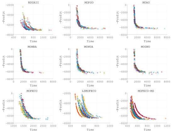
Figure 8. Plots of the non-dominated solutions in the objective space of $eil51\text{\_}n50$ obtained by nine algorithms in 15 independent runs (Pareto front obtained in each run are denoted by each color).

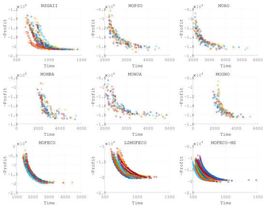
Figure 9. Plots of the non-dominated solutions in the objective space of $eil51\text{\_}n250$ obtained by nine algorithms in 15 independent runs (Pareto front obtained in each run are denoted by each color).

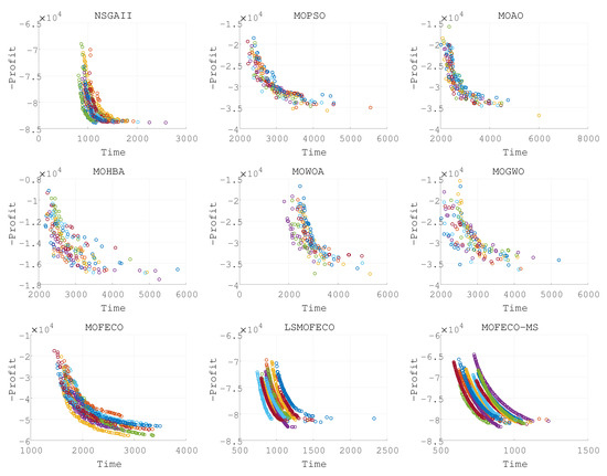
Figure 10. Plots of the non-dominated solutions in the objective space of $eil51\text{\_}n500$ obtained by nine algorithms in 15 independent runs (Pareto front obtained in each run are denoted by each color).

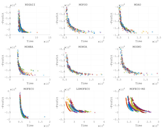
Figure 11. Plots of the non-dominated solutions in the objective space of $ch150\text{\_}n149$ obtained by nine algorithms in 15 independent runs (Pareto front obtained in each run are denoted by each color).

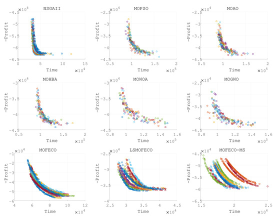
Figure 12. Plots of the non-dominated solutions in the objective space of $ch150\text{\_}n745$ obtained by nine algorithms in 15 independent runs (Pareto front obtained in each run are denoted by each color).

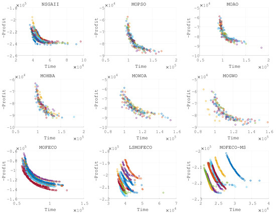
Figure 13. Plots of the non-dominated solutions in the objective space of $ch150\text{\_}n1490$ obtained by nine algorithms in 15 independent runs (Pareto front obtained in each run are denoted by each color).

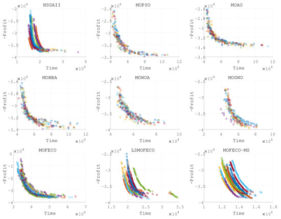
Figure 14. Plots of the non-dominated solutions in the objective space of $a280\text{\_}n279$ obtained by nine algorithms in 15 independent runs (Pareto front obtained in each run are denoted by each color).

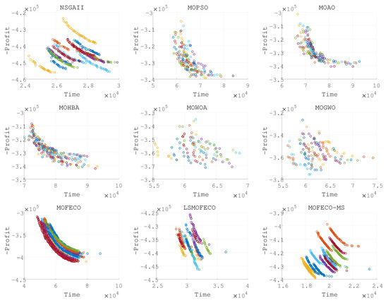
Figure 15. Plots of the non-dominated solutions in the objective space of $a280\text{\_}n1395$ obtained by nine algorithms in 15 independent runs (solutions obtained in each run are denoted by each color).

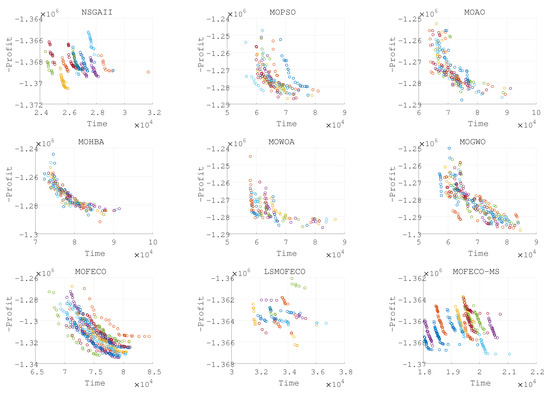
Figure 16. Plots of the non-dominated solutions in the objective space of $a280\text{\_}n2790$ obtained by nine algorithms in 15 independent runs (solutions obtained in each run are denoted by each color).

Based on the experimental results presented in Figure 8, Figure 9, Figure 10, Figure 11, Figure 12, Figure 13, Figure 14, Figure 15 and Figure 16 and the detailed metrics analysis, we can derive key insights into the performance of the MOFECO-MS algorithm compared to other competing algorithms across the various BITTP instances:

• Overall summary:

  –

  MOFECO-MS demonstrated outstanding performance across multiple instances, particularly in the HV (Hypervolume) and SP (Spread) indicators, proving its overall advantage in multi-objective optimization problems.

  –

  While MOFECO-MS did not achieve the highest PD (Pure Diversity) values in every instance, its performance remained stable and close to optimal.

  –

  The comparison charts show that MOFECO-MS consistently outperformed other algorithms in terms of solution distribution and quality across different instances, highlighting its ability to generate diverse and stable solutions.

• Specific instance analysis:

  –

  $eil{51}_{\text{\_}}n50$:

  *

  HV Indicator: MOFECO-MS achieved the best HV values across all statistical measures in 15 runs, demonstrating strong overall performance. The only exception was its variance, which was not the best, but its overall performance remained excellent.

  *

  SP Indicator: MOFECO-MS had convergence results slightly behind LSMOFECO, but the performance was very close, showing excellent capability in maintaining solution concentration and convergence.

  *

  PD Indicator: Although not the highest, MOFECO-MS still performed well, indicating strong competitiveness in diversity.

  –

  $eil51\text{\_}n250$:

  *

  HV and SP Indicators: MOFECO-MS excelled in these key indicators, showing outstanding performance in both overall quality and convergence.

  *

  PD Indicator: Second to MOFECO but still ranked highly, indicating strong diversity performance.

  –

  $eil51\text{\_}n500$:

  *

  HV Indicator: MOFECO-MS achieved the best HV values, confirming its overall performance advantage.

  *

  SP Indicator: It performed closely with LSMOFECO, showing good convergence.

  *

  PD Indicator: Second to MOFECO, but still ranked highly.

  –

  $ch150\text{\_}n149$:

  *

  HV and SP Indicators: MOFECO-MS achieved the best performance in both indicators, showing strong performance in medium-scale instances.

  *

  PD Indicator: While not the highest, it remained at a high level.

  –

  $ch150\text{\_}n1395$, $ch150\text{\_}n1490$:

  *

  HV and SP Indicators: MOFECO-MS continues to perform best in these two indicators, showing excellent performance in more complex instances.

  *

  PD Indicator: Slightly behind MOFECO but still close to optimal, indicating a good balance in diversity.

  –

  $a280\text{\_}n279$,$a280\text{\_}n1395$, $a280\text{\_}n2790$:

  *

  Performance Summary: In these instances, MOFECO-MS maintained its outstanding performance, particularly in HV and SP indicators, continuing to show the best performance. The PD indicator was close to optimal, demonstrating overall excellence.

  *

  The charts show that MOFECO-MS continues to deliver excellent distribution and high quality in these instances, demonstrating the algorithm’s robustness in large-scale problems.

• Analysis and discussion

  –

  The reason MOFECO-MS performed well across multiple runs is due to its well-balanced global exploration and local exploitation capabilities, allowing it to find high-quality solutions across different scales and complexities of TTP instances.

  –

  Convergence: MOFECO-MS’s optimization strategy effectively reduces gaps between solutions, ensuring uniform distribution along the Pareto front.

  –

  Diversity: Although MOFECO-MS did not achieve the highest PD values in some instances, it still maintained a high level of diversity, meaning it could explore a broader solution space without sacrificing quality.

  –

  Stability: MOFECO-MS demonstrated stability across multiple independent runs, indicating that its design is capable of consistently delivering high-quality outputs when addressing complex problems.

  –

  MOFECO-MS consistently performed exceptionally well across a wide range of BITTP instances, proving its potential as a powerful tool for solving complex multi-objective optimization problems. Its outstanding performance in HV and SP indicators, combined with its balanced performance in PD, makes it one of the leading algorithms in handling problems of various scales.

From the results presented in Figure 8, Figure 9, Figure 10, Figure 11, Figure 12, Figure 13, Figure 14, Figure 15 and Figure 16, it is evident that the MOFECO-MS algorithm consistently outperforms other algorithms in most of the BITTP instances, particularly in terms of Hypervolume (HV) and Spread (SP) indicators. Its strong performance can be attributed to its ability to balance exploration and exploitation effectively, ensuring both high-quality solutions and diverse coverage of the Pareto front. While it may not always achieve the highest Pure Diversity (PD) values, its performance in this area remains competitive, further demonstrating its robustness across different problem scales.

6. Conclusions and Future Work

This paper presents a Multi-objective Five-element Cycle Optimization algorithm based on Multi-strategy fusion (MOFECO-MS) for solving instances of the Bi-objective Traveling Thief Problem (BITTP). Building on the principles of the Five-element Cycle Optimization algorithm, we introduced a novel selection and update strategy that enhances the algorithm’s ability to balance global exploration and local exploitation. The algorithm’s effectiveness was demonstrated through extensive comparative evaluations across nine BITTP instances, where MOFECO-MS consistently outperformed eight leading multi-objective optimization algorithms in terms of solution quality, distribution, and convergence. The results affirm MOFECO-MS as a robust and effective approach for complex multi-objective optimization problems, particularly in scenarios requiring both precision and diversity.

For future work, we aim to explore adaptive parameter adjustment mechanisms to further improve the algorithm’s performance, particularly in terms of crossover and mutation probabilities. Additionally, we plan to investigate the incorporation of dynamic update strategies that adjust based on the evolutionary stage, which could enhance the algorithm’s ability to adapt to different problem landscapes. Another promising direction includes integrating other evolutionary operators into the update strategy and exploring the potential of co-evolution with complementary algorithms to further advance BITTP solution methodologies.

References

- Mei, Y.; Li, X.; Yao, X. On investigation of interdependence between sub-problems of the Travelling Thief Problem. Soft Comput. 2016, 20, 157–172. [Google Scholar] [CrossRef]
- Bonyadi, M.R.; Michalewicz, Z.; Barone, L. The travelling thief problem: The first step in the transition from theoretical problems to realistic problems. In Proceedings of the 2013 IEEE Congress on Evolutionary Computation, Cancun, Mexico, 20–23 June 2013. [Google Scholar]
- El Yafrani, M.; Ahiod, B. A local search based approach for solving the Travelling Thief Problem: The pros and cons. Appl. Soft Comput. 2017, 52, 795–804. [Google Scholar] [CrossRef]
- Maity, A.; Das, S. Efficient hybrid local search heuristics for solving the travelling thief problem. Appl. Soft Comput. 2020, 93, 106284. [Google Scholar] [CrossRef]
- El Yafrani, M.; Ahiod, B. Cosolver2B: An efficient local search heuristic for the travelling thief problem. In Proceedings of the 2015 IEEE/ACS 12th International Conference of Computer Systems and Applications (AICCSA), Marrakech, Morocco, 17–20 November 2015; pp. 1–5. [Google Scholar]
- Yafrani, M.E.; Martins, M.S.; Krari, M.E.; Wagner, M.; Delgado, M.R.; Ahiod, B.; Lüders, R. A fitness landscape analysis of the travelling thief problem. In Proceedings of the Genetic and Evolutionary Computation Conference, Kyoto, Japan, 15–19 July 2018; pp. 277–284. [Google Scholar]
- El Yafrani, M.; Ahiod, B. Efficiently solving the Traveling Thief Problem using hill climbing and simulated annealing. Inf. Sci. 2018, 432, 231–244. [Google Scholar] [CrossRef]
- Moeini, M.; Schermer, D.; Wendt, O. A hybrid evolutionary approach for solving the traveling thief problem. In Proceedings of the International Conference on Computational Science and Its Applications; Springer: New York, NY, USA, 2017; pp. 652–668. [Google Scholar]
- Wagner, M. Stealing items more efficiently with ants: A swarm intelligence approach to the travelling thief problem. In Proceedings of the International Conference on Swarm Intelligence; Springer: New York, NY, USA, 2016; pp. 273–281. [Google Scholar]
- Zouari, W.; Alaya, I.; Tagina, M. A new hybrid ant colony algorithms for the traveling thief problem. In Proceedings of the Genetic and Evolutionary Computation Conference Companion, Prague, Czech Republic, 13–17 July 2019; pp. 95–96. [Google Scholar]
- Laszczyk, M.; Myszkowski, P.B. A Specialized Evolutionary Approach to the bi-objective Travelling Thief Problem. In Proceedings of the 2019 Federated Conference on Computer Science and Information Systems, Leipzig, Germany, 1–4 September 2019; pp. 47–56. [Google Scholar]
- Wu, J.; Polyakovskiy, S.; Wagner, M.; Neumann, F. Evolutionary Computation plus Dynamic Programming for the Bi-Objective Travelling Thief Problem. In Proceedings of the Genetic and Evolutionary Computation Conference, Kyoto, Japan, 15–19 July 2018; pp. 777–784. [Google Scholar]
- Santana, R.; Shakya, S. Evolutionary approaches with adaptive operators for the bi-objective TTP. In Proceedings of the 2022 IEEE Symposium Series on Computational Intelligence (SSCI), Singapore, 4–7 December 2022; pp. 1202–1209. [Google Scholar] [CrossRef]
- Kumari, R.; Srivastava, K. Variable Neighbourhood Search for Bi-Objective Travelling Thief Problem. In Proceedings of the 2020 8th International Conference on Reliability, Infocom Technologies and Optimization (Trends and Future Directions) (ICRITO), Noida, India, 4–5 June 2020; pp. 47–51. [Google Scholar]
- Chagas, J.B.C.; Wagner, M. A weighted-sum method for solving the bi-objective traveling thief problem. Comput. Oper. Res. 2022, 138, 105560. [Google Scholar] [CrossRef]
- Yang, L.; Jia, X.; Xu, R.; Cao, J. An MOEA/D-ACO Algorithm with Finite Pheromone Weights for Bi-objective TTP. In Proceedings of the Data Mining and Big Data: 6th International Conference, DMBD 2021, Guangzhou, China, 20–22 October 2021; Proceedings, Part I 6. Springer: New York, NY, USA, 2021; pp. 468–482. [Google Scholar]
- Rabiei, P.; Mirghaderi, S.H.; Arias-Aranda, D. Efficiently Solving the Bi-Objective Traveling Thief Problem Using Imperialist Competitive Algorithm: Case of Small Instances. SSRN 2023. [Google Scholar]
- Blank, J.; Deb, K.; Mostaghim, S. Solving the Bi-objective Traveling Thief Problem with Multi-objective Evolutionary Algorithms. In Proceedings of the International Conference on Evolutionary Multi-Criterion Optimization, Münster, Germany, 17–19 March 2017; pp. 46–60. [Google Scholar]
- Santana, R.; Shakya, S. Dynamic programming operators for the bi-objective Traveling Thief Problem. In Proceedings of the 2020 IEEE Congress on Evolutionary Computation (CEC), Glasgow, UK, 19–24 July 2020; pp. 1–8. [Google Scholar]
- Kumari, R.; Srivastava, K. NSGAII for Travelling Thief Problem with Dropping Rate. In Proceedings of the 2023 7th International Conference on Intelligent Computing and Control Systems (ICICCS), Madurai, India, 17–19 May 2023; pp. 1647–1653. [Google Scholar]
- Chagas, J.B.C.; Blank, J.; Wagner, M.; Souza, M.J.F.; Deb, K. A non-dominated sorting based customized random-key genetic algorithm for the bi-objective traveling thief problem. J. Heuristics 2021, 27, 267–301. [Google Scholar] [CrossRef]
- Liu, M. Five-elements cycle optimization algorithm for the travelling salesman problem. In Proceedings of the International Conference on Advanced Robotics, Hong Kong, China, 10–12 July 2017; pp. 595–601. [Google Scholar]
- Polyakovskiy, S.; Mohammad Reza, B.; Markus, W.; Zbigniew, M.; Frank, N. A Comprehensive Benchmark Set and Heuristics for the Traveling Thief Problem. In Proceedings of the 2014 Annual Conference on Genetic and Evolutionary Computation, Vancouver, BC, Canada, 12–16 July 2014; pp. 477–484. [Google Scholar]
- Ye, C.; Mao, Z.; Liu, M. A Novel Multi-Objective Five-Elements Cycle Optimization Algorithm. Algorithms 2019, 12, 244. [Google Scholar] [CrossRef]
- Mao, Z.; Liu, M. A local search-based many-objective five-element cycle optimization algorithm. Swarm Evol. Comput. 2022, 68, 101009. [Google Scholar] [CrossRef]
- Deb, K.; Agrawal, S.; Pratap, A.; Meyarivan, T. A Fast Elitist Non-dominated Sorting Genetic Algorithm for Multi-objective Optimization: NSGA-II. In Proceedings of the International Conference on Parallel Problem Solving from Nature, Paris, France, 18–20 September 2000; pp. 849–858. [Google Scholar]
- Goldberg, D.E.; Lingle, R. AllelesLociand the Traveling Salesman Problem. In Proceedings of the 1st International Conference on Genetic Algorithms, Pittsburgh, PA, USA, 24–26 July 1985. [Google Scholar]
- Syswerda, G. Uniform Crossover in Genetic Algorithms. In Proceedings of the 3rd International Conference on Genetic Algorithms, Fairfax, VA, USA, 2–9 June 1989. [Google Scholar]
- Wang, K.P.; Huang, L.; Zhou, C.G.; Pang, W. Particle swarm optimization for traveling salesman problem. In Proceedings of the International Conference on Machine Learning and Cybernetics, Xi’an, China, 5 November 2003; pp. 1583–1585. [Google Scholar]
- Zitzler, E.; Thiele, L. Multiobjective Optimization Using Evolutionary Algorithms—A Comparative Case Study; Springer: Berlin/Heidelberg, Germany, 1998. [Google Scholar]
- Tian, Y.; Cheng, R.; Zhang, X.; Jin, Y. PlatEMO: A MATLAB platform for evolutionary multi-objective optimization [educational forum]. IEEE Comput. Intell. Mag. 2017, 12, 73–87. [Google Scholar] [CrossRef]
- Solow, A.; Polasky, S.; Broadus, J. On the measurement of biological diversity. J. Environ. Econ. Manag. 1993, 24, 60–68. [Google Scholar] [CrossRef]
- Coello, C.C.; Lechuga, M.S. MOPSO: A proposal for multiple objective particle swarm optimization. In Proceedings of the 2002 Congress on Evolutionary Computation, CEC’02 (Cat. No. 02TH8600), Honolulu, HI, USA, 12–17 May 2002; Volume 2, pp. 1051–1056. [Google Scholar]
- Kumawat, I.R.; Nanda, S.J.; Maddila, R.K. Multi-objective whale optimization. In Proceedings of the TENCON 2017—2017 IEEE Region 10 Conference, Penang, Malaysia, 5–8 November 2017; pp. 2747–2752. [Google Scholar]
- Lu, C.; Xiao, S.; Li, X.; Gao, L. An effective multi-objective discrete grey wolf optimizer for a real-world scheduling problem in welding production. Adv. Eng. Softw. 2016, 99, 161–176. [Google Scholar] [CrossRef]
- Mohammed Hamouda, A.; Ahmed Tijani, S.; Salah, K.; Habeeb Bello, S.; Monier, H.; Mokhtar, S. Single-and multi-objective modified aquila optimizer for optimal multiple renewable energy resources in distribution network. Mathematics 2022, 10, 2129. [Google Scholar] [CrossRef]
- Papasani, A.; Devarakonda, N. A novel feature selection algorithm using multi-objective improved honey badger algorithm and strength pareto evolutionary algorithm-II. J. Eng. Res. 2022, 11, 71–83. [Google Scholar] [CrossRef]
Disclaimer/Publisher’s Note: The statements, opinions and data contained in all publications are solely those of the individual author(s) and contributor(s) and not of MDPI and/or the editor(s). MDPI and/or the editor(s) disclaim responsibility for any injury to people or property resulting from any ideas, methods, instructions or products referred to in the content. |
© 2024 by the authors. Licensee MDPI, Basel, Switzerland. This article is an open access article distributed under the terms and conditions of the Creative Commons Attribution (CC BY) license (https://creativecommons.org/licenses/by/4.0/).