Enhancing Weather Forecasting Integrating LSTM and GA

Abstract

Several sectors, such as agriculture and renewable energy systems, rely heavily on weather variables that are characterized by intermittent patterns. Many studies use regression and deep learning methods for weather forecasting to deal with this variability. This research employs regression models to estimate missing historical data and three different time horizons, incorporating long short-term memory (LSTM) to forecast short- to medium-term weather conditions at Quinta de Santa Bárbara in the Douro region. Additionally, a genetic algorithm (GA) is used to optimize the LSTM hyperparameters. The results obtained show that the proposed optimized LSTM effectively reduced the evaluation metrics across different time horizons. The obtained results underscore the importance of accurate weather forecasting in making important decisions in various sectors.

1. Introduction

Weather variables play a vital role in many sectors and activities, affecting various aspects of our daily lives. From aviation to energy production, weather conditions have a significant impact on the performance and results of various sectors. Agriculture and renewable energy production are two sectors that are highly dependent on weather variables [1].

Weather variability presents significant challenges related with the variability and unpredictability of the data, making it difficult to rely on consistent patterns. Weather forecasting plays an important role in improving the performance and efficiency of different sectors, including agriculture, energy, and transportation [2,3]. However, there are some problems associated with weather forecasts that can affect their accuracy such as traditional forecasting methods may struggle to accurately predict sudden changes, leading to less reliable weather forecasts; historical data can be incomplete or inaccurate, impacting the ability to model future conditions accurately; weather variables can have complex iterations between them and capturing these interactions in forecasting models is challenging, often requiring sophisticated algorithms and computational resources.

In fact, the accuracy and reliability of weather forecasts have a huge impact on decision making, enabling effective planning, risk mitigation, and optimization of operations. For example, understanding and accurately predicting weather variables is critical to optimizing renewable energy production, reducing costs and minimizing environmental impact. By accurately forecasting weather conditions, grid operators can anticipate fluctuations in renewable energy output and plan for backup power sources or storage solutions to maintain a reliable supply of electricity.

In the agricultural sector, weather variables play a crucial role in shaping farming practices, yield forecasting, and crop management. Farmers rely on a combination of weather variables such as temperature, rainfall, humidity, and wind patterns to make informed decisions about planting, irrigation, and harvesting. In fact, understanding weather patterns allows farmers to optimize their operations, mitigate risk, and ensure the overall health and productivity of their crops. On the other hand, solar and wind energy production is highly dependent on weather conditions, which determine the availability and efficiency of these sustainable energy systems. Karevan and Suykens [4] emphasized the importance of weather forecasting in these areas because of its impact on productivity, resource allocation, and risk management. They proposed a transductive long short-term memory (T-LSTM) method to extract local information in weather time series.

Regarding the historical data used in forecasts, missing values affect the accuracy of forecasts. For this reason, it is important use resourceful and flexible techniques. Van Buuren [5] emphasized the importance of addressing missing data in statistical analysis, and highlighted the advantages of the multiple imputation (MI) approach and Doreswamy et al. [6] discussed the significance of handling missing data in weather datasets, which is crucial for accurate climate forecasting impacting various sectors. The paper proposes a new technique for addressing missing values in weather data using machine learning algorithms, such as kernel ridge regression, linear regression, random forest, or support vector machine (SVM) imputation. In this paper, regarding the characteristics of the places under studies, we chose to use regression methods to estimate missing values due to their ability to leverage relationships between variables.

Long short-term memory (LSTM) networks are a type of recurrent neural network (RNN) designed to model sequential data, making them highly suitable for weather forecasting. Since, weather data involve complex, non-linear interactions between various variables, such as, wind speed or direction, LSTMs are capable of modeling these non-linear relationships more effectively than traditional linear models, but also can effectively capture long-term dependencies in sequential data, like the temperature [7,8].

The accuracy of LSTM forecasts can be influenced by various factors. Viedma et al. [9] highlight the impact of classical time series pre-processing methods, with seasonal-component removal being particularly effective, the importance of data quality, model architecture, and hyperparameter tuning. The use of genetic algorithms (GA) to optimize the parameters of LSTM forecasting methods has been shown to significantly improve their accuracy. The authors in [10,11] both demonstrate the effectiveness of this approach in short-term load forecasting, with the first achieving a small mean absolute percentage error and the second improving prediction accuracy by 63%. Bouktif et al. [12] extend this to medium- and long-term forecasting, highlighting the ability of the LSTM model, optimized with GAs, to capture the characteristics of complex time series and reduce forecasting errors. These studies collectively underscore the importance of using GAs to enhance the accuracy of LSTM forecasting methods.

With this in mind, the main objective of this work was to analyze short- to medium-term weather forecasting. To this end, combined methods of regression and LSTM techniques were proposed and later evaluated to assess their accuracy and efficiency. Therefore, the main contributions of this work are (1) estimation of historical data considering regression techniques; (2) short- and medium-term weather prediction using LSTM networks; (3) evaluation of the model’s forecasting task considering specific metrics.

The subsequent parts of the paper are organized as follows: Section 2 presents some work already developed regarding the proposed theme; Section 3 describes the sites under study, the methodology, presenting the methods considered, their mathematical formulation, the evaluation metrics used, and the case studies considered; Section 4 presents the main results obtained, discussing the relevant points according to the results of accuracy and efficiency of the evaluation metrics; finally, Section 5 presents the main conclusions of the paper and future work.

2. Related Work

Several works have studied the importance and accuracy of weather forecasting in the literature. Regression and machine learning models are two of the main techniques used, and some of the work is described below. Regression models are a type of statistical model commonly used in forecasting techniques. In effect, statistical models use historical data to predict new values by adjusting the parameters of the model by analyzing the differences between the observed and predicted values [13]. Linear regression models analyze the linear relationship between dependent and independent variables, improving the accuracy and reducing the computational time of the model [14]. According to Jassena and Kovoor [1], there are two main types of linear regression models: simple and multiple. Simple linear regression describes the linear relationship between one dependent variable and one independent variable. On the other hand, multiple linear regression (MLR) analyses the linear relationship between a dependent variable and more than one independent variable. In Ansarifar et al. [15], different regression models such as MLR or least absolute shrinkage and selection operator (LASSO) regression were proposed to continuously update weather and management data with future scenarios to obtain weekly crop yield forecasts. The results showed that the proposed model achieved accurate and timely crop yield predictions compared to machine learning algorithms. In Barriguinha et al. [16], a systematic review was presented that analyzed multiple linear regression (MLR), as well as partial least squares regression, and random forest regression, to estimate grape and wine production by predicting climatic conditions such as temperature or precipitation. Overall, the paper highlighted that the accuracy and reliability of regression models depend on the quality and quantity of data, the selection of appropriate predictors, and the validation of the model, but can be useful for estimating vineyard yield.

Similarly, in the renewable energy context, regression methods are often used to predict climate variables. Amir and Zaheeruddin [17] analyzed the short-term prediction of solar radiation and wind speed using regression models to assess the linear relationship between the variables. The proposed model can effectively capture the dependencies between the variables with an accuracy of 98.2%. Ridge regression models have been proposed in [18,19] to predict solar radiation and wind speed. In the former, the main objective was to reduce the problems associated with the intermittency of these variables, thus reducing the associated forecast errors. The results showed that the proposed model had a correlation coefficient of 0.903 and was able to improve the accuracy and generalization of the forecasts.

As regression methods are not as efficient at dealing with non-linear data and high variability, machine learning methods, in particular deep learning (DL), are emerging as a solution [20]. In fact, DL can automatically learn features from data, instead of considering traditional selection techniques [21].

Extreme gradient boosting (XGBoost) is a powerful and versatile machine learning algorithm that has demonstrated exceptional performance in various applications. It is particularly effective in modeling complex systems, achieving high prediction accuracy, and handling large-scale data. It has been successfully applied in various fields, including weather forecasting for agriculture and renewable energy production. Phan et al. and Wadhwa and Tiwary [22,23] demonstrated the effectiveness of XGBoost in improving the accuracy of short-term solar power and wind power forecasts. Another useful method is transformer networks. Transformer networks have been shown to significantly improve the accuracy of weather variable forecasts. In [24], a hybrid system was introduced, H-Transformer, which outperformed other models in predicting renewable energy production. Nascimento et al. [25] presented a transformer-based model with wavelet transform for wind speed and wind energy forecasting, showing superior performance compared to a baseline LSTM model. However, Walczewski et al. [26] found that the performance of transformer-based models varied depending on the specific forecasting task and the data provided, with the LSTM model outperforming all others in predicting onshore wind and photovoltaic energy.

Recurrent neural networks (RNNs) are widely used in weather forecasting due to their computational power, sophisticated algorithms, and storage capacity [27]. However, RNNs have a drawback when it comes to handling long-term correlations, as they suffer from gradient loss and explosion [28]. One solution to this problem is to use LSTMs, which are a type of RNN-based model. They excel at solving both short- and long-term problems by effectively predicting and storing temporal data [29,30].

Thirunavukkaras et al. [31] proposed an LSTM method to efficiently predict solar radiation 15 min ahead in certain areas with high intermittency. The proposed model outperformed other models such as auto-regressive or persistence by about 40%, improving the accuracy and efficiency of the model. Similarly, short-term wind energy forecasts are prone to accuracy problems due to the intermittent nature of wind [32]. Thus, an LSTM was proposed to deal with linear and non-linear components of time series of wind power generated by offshore turbines. The proposed model increased the prediction accuracy by 13.2% compared to a baseline model.

Finally, in the agricultural sector, LSTM networks are also being considered for weather forecasting. For example, in Salehin et al. [33] an LSTM was used to accurately determine the amount of rainfall needed to increase crop yields and reduce agricultural costs. The model takes into account weather variables such as temperature, humidity, and wind speed to make predictions and reports an accuracy of 76% in predicting rainfall.

3. Data and Methods

The methodology developed in this paper involves a two-step approach: first, regression models are employed to estimate missing values in the input dataset; second, LSTM networks are utilized to forecast weather variables for a specified future horizon. The dataset and methods employed are detailed below.

3.1. Dataset

This work considers weather data collected from two locations: Pinhão town and Quinta de Santa Bárbara. Quinta de Santa Bárbara is located at coordinates 41.172753° N, −7.549335° W. The data were collected from a sensor located in Quinta de Santa Bárbara between September 8 and 30 December 2022, totaling a sampling length of 114 days. However, for a more robust forecast, a larger input dataset is advantageous to improve the validation, stability, generalization, and accuracy of the forecasts. To this end, climate data from the Portuguese Institute for Sea and Atmosphere (IPMA) station, located at coordinates 41.172775° N, −7.548972° W, were also used, as it is in the same geographical area as the study site, as shown in Figure 1. This additional dataset comprises a sample of 4748 days, covering the period from 1 January 2010, to 31 December 2022.

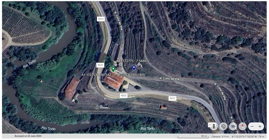
Figure 1. Location of the studied site.

When analyzing the data from Pinhão, reading errors of the sensor were eliminated for each of the variables studied. Since the data were collected daily, any outlier value for a particular day was replaced with the average value for that day in the other years.

In turn, the range of values measured at Quinta de Santa Bárbara was presented at 15-min intervals. Thus, for each of the variables studied, the hourly values were averaged, and then, the average of these values was used to obtain the daily values.

3.2. Forecasting with Regression Models

Given the data from the two locations, it was necessary to find a relation between the variables measured at Pinhão and Quinta de Santa Bárbara, in order to predict the missing values from the measurements at Quinta de Santa Bárbara. The regression methods selected for this study included MLR [19], LASSO, and ridge regressions [34,35].

The MLR is given by

$$Y={\beta }_0+{\beta }_1·x_1+{\beta }_2·x_2+\cdots +{\beta }_n·x_n$$

(1)

where Y is the dependent variable, which corresponds to the missing values between 2010 and 2022 at Quinta de Santa Bárbara; $x_i,i=1,2,\dots ,n$ are the independent variables, corresponding to the measurements in Pinhão; ${\beta }_0$ is the constant term, ${\beta }_i$ with $i=1,2,\dots$; and n are the regression coefficients. For the LASSO and ridge models, the L1 and L2 regularization terms are added to Equation (1). Therefore, in order to take into account the advantages of these three methods, a combined model was considered to predict the missing data.

3.3. Forecasting with Long Short-Term Memory

Once the data from Quinta de Santa Bárbara between 2010 and 2022 had been estimated, LSTM networks were used to predict the variables under study for the short- to medium-term future.

According to [36], LSTM neural networks consist of three key components: input gate $i_t$, forgetting gate $f_t$, and output gate $o_t$. These components regulate the storage and removal of information within the network. This makes it possible to control when a memory unit retains previous information and maintains a constant error during the back-propagation process [27]. LSTMs have a cell state and a hidden state. The cell state propagates through the input and output sequences, while the temporal information is processed by the three gates responsible for incorporating, filtering, and selecting relevant information for output. The mathematical formulation outlining the LSTM structure can be represented by Equations (2)–(7) [32]:

$$\begin{array}{c}{f}_t=\sigma (W_f[h_{t-1},x_t]+b_f)\end{array}$$

(2)

$$\begin{array}{c}{i}_t=\sigma (W_i[h_{t-1},x_t]+b_i)\end{array}$$

(3)

$$\begin{array}{c}o\left(t\right)=\sigma (W_o[h_{t-1},x_t]+b_o)\end{array}$$

(4)

$$\begin{array}{c}{c}_t^{\prime }=tanh(W_s[h_{t-1},x_t]+b_s)\end{array}$$

(5)

$$\begin{array}{c}{c}_t=c_{t-1}\odot f_t+g_t\odot i_t\end{array}$$

(6)

$$\begin{array}{c}{h}_t=tanh\left(c_t\right)\odot i_t\end{array}$$

(7)

where $[h_{t-1},x_t]$ represents the input signal, which consists of the input neuron $x_t$ at time t and the cell state $c_{t-1}$ at time $t-1$. $W_f$, $W_i$, $W_o$, and $W_s$ denote the weights that connect the forgetting gate, input gate, output gate, and cell state, respectively, to the input signal. $b_f$, $b_i$, $b_o$, and $b_s$ represent the biases, and $\sigma$ denotes the activation function. Additionally, $h_t$ corresponds to the output value at time t. The operator ⊙ represents the element-wise multiplication.

In this paper, instead of using tanh as the activation function, the rectified linear unit (ReLU) was considered. In brief, it returns the input value if it is positive, and zero if it is negative, introducing non-linearity to the model.

Since the hyperparameters that characterize an LSTM affect the accuracy of forecasts, a GA was considered to improve the performance. The fitness function uses the mean square error (MSE) between the predicted and observed values to guide the GA in finding the best LSTM parameter combination.

3.4. Genetic Algorithm

Genetic algorithm (GA) is a search and optimization technique inspired by natural selection. The GA simulates the evolution of a population of chromosomes, each one representing a potential solution to a problem. These chromosomes or individuals are scored according to their fitness, which determines their likelihood of being selected for reproduction. During the reproduction phase, genes from high-performing chromosomes are usually selected, combined, and mutated to produce offspring “solutions” potentially better than their progenitors. This iterative selection, reproduction, and mutation process allows the population to evolve towards increasingly optimal solutions over time. Genetic algorithms are powerful methods for solving problems, particularly where no traditional algorithm exists or where traditional optimization methods struggle due to large solution spaces and intricate variable relationships.

3.5. Evaluation Metrics

The coefficient of determination $R^2$ was used to evaluate the regression models, and the MSE, root mean square error (RMSE), and mean absolute error (MAE) were considered to evaluate the LSTM models.

The statistical measure $R^2$, where $0\le R^2\le 1$, assess the goodness of fit of the model and measure the predictive power of the independent variables, Equation (8). The higher the $R^2$ value, the better the model fits the data.

$$R^2=1-\frac{S{S}_{res}}{S{S}_{tot}}$$

(8)

where n is the sample size, $S{S}_{res}$ is the sum of squared residuals, $S{S}_{res}={\sum }_{i=1}^n{(y_i-y_i^{\prime })}^2$, $S{S}_{tot}$ is the sum of squared differences between the observed values and the mean of observed values, $S{S}_{tot}={\sum }_{i=1}^n{(y_i-\overline{y})}^2$, $y_i$ is the observed value, and $y_i^{\prime }$ is the predicted value.

The MSE measures the average of the squared differences between the observed and predicted values:

$$\mathrm{MSE}=\frac{1}{n}\sum _{i=1}^n{(y_i-y_i^{\prime })}^2$$

(9)

The MAE measures the average of the absolute differences between observed and predicted values:

$$\mathrm{MAE}=\frac{1}{n}\sum _{i=1}^n|y_i-y_i^{\prime }|$$

(10)

Finally, the RMSE takes into account the square root of the differences between the observed and predicted values:

$$\mathrm{RMSE}=\sqrt{\frac{1}{n}\sum _{i=1}^n{(y_i-y_i^{\prime })}^2}$$

(11)

These metrics therefore play an important role in the case studies that have been developed, as they make it possible to compare the different results obtained. They were calculated considering the forecast and observed data from the testing dataset for the time range of predictions.

Figure 2 shows the methodology applied in this paper. Considering the two locations, the datasets were pre-processed. After that, regression models were used to estimate the missing values for Quinta de Santa Bárbara between 2010 and 2022, considering the data obtained from Pinhão. After obtaining the new dataset for Quinta de Santa Bárbara, an LSTM network was considered to forecast short- to medium-term weather variables. A GA was also considered to optimize the hyperparameters of the network. Finally, the proposed evaluation metrics allow us to evaluate and compare the forecast results of each proposed network.

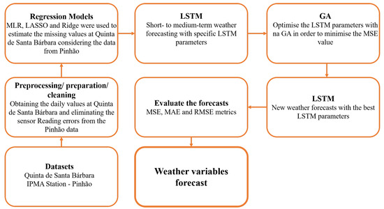
Figure 2. Applied methodology, considering the datasets and methods used for short- to medium-term weather forecasting.

The following cases have been proposed to evaluate the accuracy of weather forecasting using LSTM networks for short- and medium-term horizons:

• Case I: Short- and medium-term forecasting using LSTM.
• Case II: Short- and medium-term forecasting using an optimized LSTM with a GA.

4. Results and Discussion

This section presents the results obtained in relation to the estimated values and the forecast weather variables. Regression models were used to estimate and fill the missing data for Quinta de Santa Bárbara. Subsequently, LSTM networks were employed to forecast weather variables for 3 to 15 days.

The models used in this study were built using the Python 3.11 programming language [37]. The LSTM networks were implemented using the TensorFlow tool [38], a widely used framework for deep learning applications in Python, and the regression models were developed using the Scikit-learn library [39].

4.1. Forecasting with Regression Models

The linear relation between the two sites was analyzed for each of the variables in the time interval common to both sets of data, i.e., between 8 September and 30 December 2022.

To take advantage of the regression techniques described in Section 3, a combined model was developed to predict missing data. The measurements recorded at Quinta de Santa Bárbara were used as dependent variables, while those from Pinhão were considered as independent variables.

Figure 3 shows the scatter plots of the observed values (blue dots) and the trend line that fits the data.

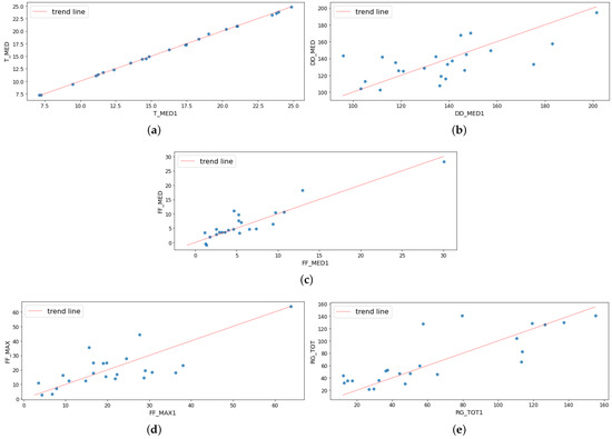
Figure 3. Linear relationship between the values observed in Pinhão and Quinta de Santa Bárbara: (a) daily average temperature, (b) daily wind direction, (c) daily average wind speed, (d) daily instantaneous wind speed, and (e) daily solar radiation.

For the daily average temperature ($F{F}_{MED}$), the values observed in the two locations have a strong linear relation. In turn, for the other variables, the observed values are dispersed around the trend line, which also shows that the proposed model is capable of making accurate predictions for these variables. However, in order to verify whether the MLR model fits the dataset, we evaluated the $R^2$ values and its residuals.

Table 1 shows the $R^2$ values for each of the variables under study. Analyzing the $R^2$ values, it can be seen that they are relatively high for all the variables except the daily wind direction ($D{D}_{MED}$), which had a value less than 0.5.

Table 1. $R^2$ values for each dependent variable studied.

Variable	Description	${\mathit{R}}^2$
T_MED	Daily average temperature	0.999
DD_MED	Daily wind direction	0.477
FF_MED	Daily average wind speed	0.821
FF_MAX	Daily instantaneous wind speed	0.686
RG_TOT	Daily solar radiation	0.754

The residuals of an MLR are analyzed by constructing scatter plots, which are a useful tool for evaluating the fit of these models. Its representation consists of a graph, where the y-axis shows the normalized residuals and the x-axis shows the normalized residuals; Figure 4. In general, the results are randomly dispersed, with a mean of zero and a constant variance, as intended.

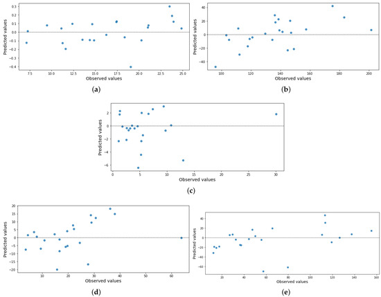
Figure 4. Graphical representation of MLR residuals: (a) daily average temperature, (b) daily wind direction, (c) daily average wind speed, (d) daily instantaneous wind speed, and (e) daily solar radiation.

Having these results, the p-values of the coefficients were analyzed to determine whether a given independent variable had a significant effect on the dependent variables. Therefore, the p-values were analyzed for each of the dependent variables and the coefficients that did not meet the condition $(P>|t\left|\right)<0.05$ were excluded. Once the coefficients had been excluded, the best regression method for predicting each variable was chosen from among the MLR, ridge, and LASSO methods. Table 1 also shows the values of the coefficients of determination ($R^2$) for the new regression methods chosen.

Table 2 shows the method used for each variable, as well as the coefficients used to calculate the values corresponding to each variable between 2010 and 2022 in Quinta de Santa Bárbara. It can also be seen that the dependent variables do not depend on all the independent variables. This means that for each variable to be calculated, the methods select the variables that are highly correlated with the variable to be determined.

Table 2. Coefficients for the calculation of dependent variables.

Variable	Method	Coefficients					Intercept
		${\mathit{T}}_{\mathit{MED}\mathbf{1}}$	${\mathit{DD}}_{\mathit{MED}\mathbf{1}}$	${\mathit{FF}}_{\mathit{MED}\mathbf{1}}$	${\mathit{FF}}_{\mathit{MAX}\mathbf{1}}$	${\mathit{RG}}_{\mathit{TOT}\mathbf{1}}$
$T_{MED}$	Linear	1.0190	0	0	0	−0.0032	−0.1887
$D{D}_{MED}$	LASSO	0	0	24.9277	0	0	96.7312
$F{F}_{MED}$	Ridge	0	0.0124	7.7472	0	0	−7.2055
$F{F}_{MAX}$	LASSO	0	0	7.2770	1.6848	0	−5.3412
$R{G}_{TOT}$	Linear	1.1333	0.0957	0	0	0.4822	−22.3257

Finally, using the coefficients provided in Table 2, the mathematical models to calculate the predicted daily values for each variable are given by Equations (12)–(16).

$$\begin{array}{c}{T}_{MED}=-0.1887+1.0190·T_{MED1}-0.0032·R{G}_{TOT1}\end{array}$$

(12)

$$\begin{array}{c}D{D}_{MED}=96.7312+24.9277·F{F}_{MED1}\end{array}$$

(13)

$$\begin{array}{c}F{F}_{MED}=-7.2055+0.0124·D{D}_{MED1}-7.7472·F{F}_{MED1}\end{array}$$

(14)

$$\begin{array}{c}F{F}_{MAX}=-5.3412+7.277·F{F}_{MED1}+1.6848·F{F}_{MAX1}\end{array}$$

(15)

$$\begin{array}{c}R{G}_{TOT}=-22.3257+1.1333·T_{MED1}+0.0957·D{D}_{MED1}+0.4822·R{G}_{TOT1}\end{array}$$

(16)

where $T_{MED}$ is the predicted average temperature, $D{D}_{MED}$ is the predicted average wind direction, $F{F}_{MED}$ is the predicted average wind speed, $F{F}_{MAX}$ is the predicted maximum instant wind speed, and $R{G}_{TOT}$ is the predicted solar radiation for Quinta de Santa Bárbara, and $T_{MED1}$, $D{D}_{MED1}$,$F{F}_{MED1}$, $F{F}_{MAX1}$, and $R{G}_{TOT1}$ are the correspondent weather variables observed in Pinhão.

Finally, the input dataset was divided into training, validation, and testing sets. The main purpose of selecting these datasets is to assess the accuracy of the models’ performance and also to ensure that they can be generalized to new data. For the variables under study, the values were divided into training, validation, and testing sets, with a split of 70%, 15%, and 15%, respectively, as shown in Figure 5.

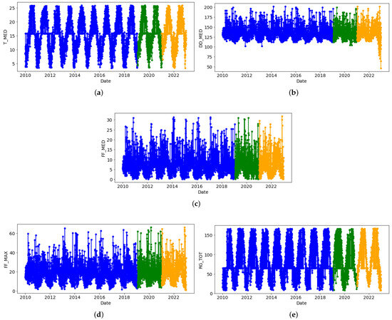
Figure 5. Train (blue), validation (green), and testing (yellow) sets: (a) daily average temperature, (b) daily wind direction, (c) daily average wind speed, (d) daily instantaneous wind speed, and (e) daily solar radiation.

4.2. Case I

In this case, each variable was forecast for 3 to 15 days, using an LSTM with specific hyperparameters characterized in Table 3. Each LSTM network had a ReLU activation function, a dense layer with 1 neuron, to obtain the output value, a dropout layer equal to 0.2, with 10 neurons, and they were optimized using Adam optimization with a learning rate of 0.001 in order to minimize the MSE.

Table 3. LSTM’s parameters.

Parameter	Value
Number of LSTM layers	1
Number of LSTM units	50
Batch size	32
Number of epochs	40

Figure 6, Figure 7 and Figure 8 show the results for the 3-, 7-, and 15-day forecasts, respectively. For each variable, the last 15 days of the test set and the predicted values for that period are also shown. In general, the predicted variables showed a similar behavior for all time periods, without significant fluctuations compared to the testing data.

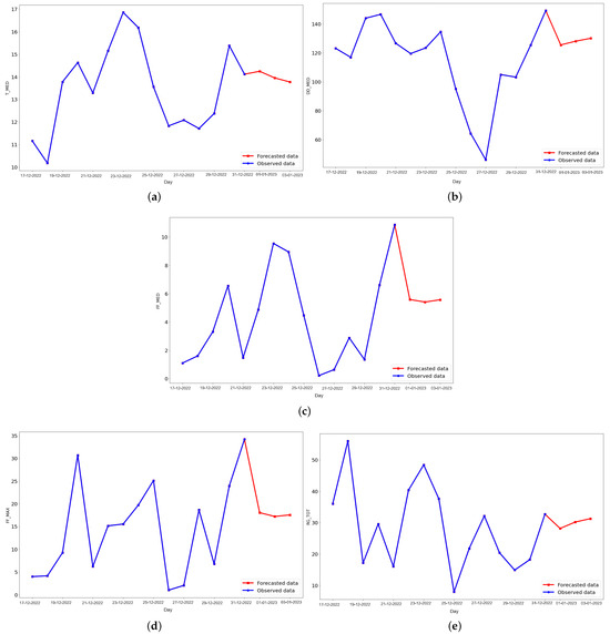
Figure 6. Last 15 days of the testing set (blue) and the predicted data (red) for 3 days ahead in the future for (a) daily average temperature, (b) daily average wind direction, (c) daily average wind speed, (d) daily instant wind speed, and (e) daily solar radiation predicted values (red), using an LSTM.

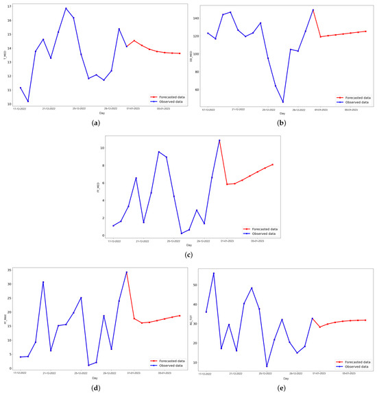
Figure 7. Last 15 days of the testing set (blue) and the predicted data (red) for 7 days ahead in the future for (a) daily average temperature, (b) daily average wind direction, (c) daily average wind speed, (d) daily instant wind speed, and (e) daily solar radiation predicted values (red), using an LSTM.

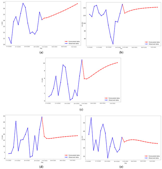
Figure 8. Last 15 days of the testing set (blue) and the predicted data (red) for 15 days ahead in the future for (a) daily average temperature, (b) daily average wind direction, (c) daily average wind speed, (d) daily instant wind speed, and (e) daily solar radiation predicted values (red), using an LSTM.

4.3. Case II

In this case, the LSTM hyperparameters were optimized with a GA method. The purpose of using this algorithm was to find the best LSTM hyperparameters that minimize the MSE of the network (Table 4). Table 5 shows the GA parameters used in this paper.

Table 4. Range of LSTM hyperparameters.

Parameter	Value
Number of LSTM layers	[1, 3]
Number of LSTM units	[50, 150]
Batch size	[16, 64]
Number of epochs	[20, 40]

Table 5. Genetic algorithm parameters.

Parameter	Value
Maximum number of iterations	5
Population size	10
Mutation rate	0.1
Elit rate	0.1
Crossover rate	0.5
Parents portion	0.3
Crossover type	Two point

Table 6 shows the LSTM hyperparameter optimization results for each variable. These results correspond to the parameters that minimize the MSE metric for each variable, according to the time period of the forecasts.

Table 6. Optimization results, case II.

	Variable	LSTM Layers	LSTM Units	Batch Size	Epochs
3 days	T_MED	3	87	49	34
	DD_MED	2	70	38	20
	FF_MED	3	98	50	27
	FF_MAX	3	50	17	21
	RG_TOT	1	76	41	31
7 days	T_MED	1	86	34	39
	DD_MED	2	91	21	21
	FF_MED	3	57	31	21
	FF_MAX	2	72	16	30
	RG_TOT	1	116	16	30
15 days	T_MED	1	118	31	30
	DD_MED	2	120	20	39
	FF_MED	2	124	54	29
	FF_MAX	3	134	25	20
	RG_TOT	2	109	42	32

Figure 9, Figure 10 and Figure 11 show the prediction results for case II. In general, the behavior of each variable is different for each time period chosen. In this case, the predicted values behave similarly to the observed data, with a more fluctuating shape than in case I.

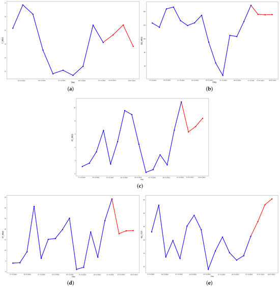
Figure 9. Last 15 days of the testing set (blue) and the predicted data (red) for 3 days ahead in the future for (a) daily average temperature, (b) daily average wind direction, (c) daily average wind speed, (d) daily instant wind speed, and (e) daily solar radiation predicted values (red), using an optimized LSTM.

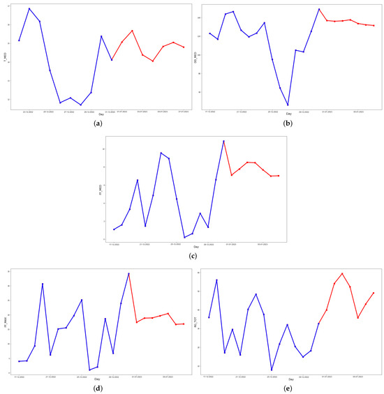
Figure 10. Last 15 days of the testing set (blue) and the predicted data (red) for 7 days ahead in the future for (a) daily average temperature, (b) daily average wind direction, (c) daily average wind speed, (d) daily instant wind speed, and (e) daily solar radiation predicted values (red), using an optimized LSTM.

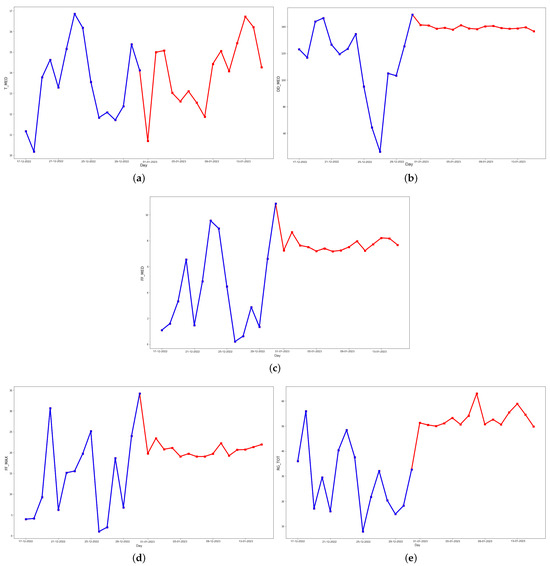
Figure 11. Last 15 days of the testing set (blue) and the predicted data (red) for 15 days ahead in the future for (a) daily average temperature, (b) daily average wind direction, (c) daily average wind speed, (d) daily instant wind speed, and (e) daily solar radiation predicted values (red), using an optimized LSTM.

4.4. Results Discussion

The evaluation metrics obtained for each proposed case were compared with two benchmark methods: XGBoost and transformer. Similarly to the proposed cases, a GA was also applied to these methods. The average numerical results obtained for each case and for the benchmark method, are presented in Table 7. The evaluation metrics represent each metric’s average daily value according to the time range studied.

Table 7. Average evaluation metrics for climatic variables by each scenario and benchmark method.

		3 Days
		T_MED	DD_MED	FF_MED	FF_MAX	RG_TOT
Case I	MSE	0.0182	0.1512	0.1512	0.3555	0.0126
	MAE	0.1266	0.3756	0.575	0.5811	0.1014
	RMSE	0.1348	0.3888	0.6166	0.5962	0.1123
Case II	MSE	0.0453	0.0082	0.0085	0.0648	0.0071
	MAE	0.1926	0.0846	0.0863	0.2306	0.0733
	RMSE	0.2129	0.0903	0.0924	0.2545	0.0841
XGBoost	MSE	45.9822	307.0847	33.0072	102.5079	3432.2502
	MAE	5.7409	13.2791	4.3613	7.8988	51.9629
	RMSE	6.781	17.5238	5.7452	10.1246	58.5854
XGBoost-GA	MSE	46.8364	352.1824	33.6135	119.3655	3208.583
	MAE	5.7277	14.1451	4.5121	8.4562	50.3719
	RMSE	6.8437	18.7665	5.7977	10.9255	56.6444
Transformer	MSE	0.0026	0.0061	0.0053	0.0305	0.001
	MAE	0.0415	0.0696	0.0612	0.1622	0.0318
	RMSE	0.0506	0.07832	0.0726	0.1747	0.0321
Transformer-GA	MSE	0.0024	0.0057	0.0048	0.0253	0.0011
	MAE	0.0412	0.0655	0.0575	0.1393	0.0312
	RMSE	0.0492	0.0757	0.0695	0.1589	0.0335
		7 days
		T_MED	DD_MED	FF_MED	FF_MAX	RG_TOT
Case I	MSE	0.0078	0.0867	0.2034	0.1985	0.0205
	MAE	0.0778	0.2505	0.3774	0.385	0.1205
	RMSE	0.0882	0.2944	0.451	0.4456	0.1433
Case II	MSE	0.003	0.0328	0.0681	0.1633	0.0069
	MAE	0.0778	0.1596	0.2211	0.3682	0.0708
	RMSE	0.0882	0.1812	0.261	0.4042	0.08291
XGBoost	MSE	45.9822	307.0847	33.0072	102.5079	3432.2502
	MAE	5.7409	13.2791	4.3613	7.8988	51.9629
	RMSE	6.781	17.5238	5.7452	10.1246	58.5854
XGBoost-GA	MSE	46.9001	352.1685	33.6112	115.7482	3333.5516
	MAE	5.7328	14.1547	4.5106	8.4012	51.0867
	RMSE	6.8484	18.7662	5.7975	10.7586	57.7369
Transformer	MSE	0.003	0.034	0.0052	0.0291	0.0035
	MAE	0.0518	0.1569	0.0643	0.1513	0.0502
	RMSE	0.0548	0.1896	0.072	0.1706	0.0591
Transformer-GA	MSE	0.0037	0.0395	0.0059	0.0285	0.0024
	MAE	0.0546	0.1633	0.0675	0.1439	0.0392
	RMSE	0.0611	0.1988	0.0766	0.1689	0.0493
		15 days
		T_MED	DD_MED	FF_MED	FF_MAX	RG_TOT
Case I	MSE	0.0081	0.047	0.107	0.1116	0.0239
	MAE	0.073	0.1528	0.2305	0.2623	0.1368
	RMSE	0.0898	0.2166	0.3271	0.3341	0.1547
Case II	MSE	0.005	0.0337	0.0818	0.1254	0.0042
	MAE	0.0602	0.1408	0.2179	0.2919	0.054
	RMSE	0.0706	0.1835	0.286	0.3542	0.0647
XGBoost	MSE	45.9822	307.0847	33.0072	102.5079	3432.2502
	MAE	5.7409	13.2791	4.3613	7.8988	51.9629
	RMSE	6.781	17.5238	5.7452	10.1246	58.5854
XGBoost-GA	MSE	46.7768	352.1688	33.6143	118.2286	3316.611
	MAE	6.8394	18.7662	5.7978	10.8733	57.59
	RMSE	5.7214	14.1526	4.5125	8.4312	50.9951
Transformer	MSE	0.0057	0.0169	0.0082	0.0324	0.0044
	MAE	0.0575	0.1065	0.0783	0.1521	0.0563
	RMSE	0.0754	0.1301	0.0905	0.1799	0.0665
Transformer-GA	MSE	0.0059	0.0242	0.0053	0.0245	0.0046
	MAE	0.0634	0.1554	0.0726	0.1566	0.0677
	RMSE	0.077	0.1554	0.0726	0.1566	0.0676

Regarding the predicted variables, it can be seen that they generally have good results for the metrics, with values less than 1, which indicates that the proposed models are capable of predicting climate variables in the short and medium term. In general, when comparing the case studies considered, it can be seen that optimizing the characteristic parameters of the LSTM improved the metric values for all prediction horizons. The use of the GA minimized the MSE value for all variables, regardless of the horizon considered. For example, for a 3-day forecast, the MSE, MAE, and RMSE values for temperature (T_MED) decreased by 97%, 81%, and 81%, respectively, for mean wind speed (FF_MED) by 94%, 85%, and 85%, and for solar radiation (RG_TOT) by 44%, 28%, and 25%, respectively. On the other hand, for a 7-day forecast horizon, the values for T_MED decreased by 63%, 34%, and 52%, for FF_MED by 67%, 41%, and 42% and for RG_TOT by 66%, 41%, and 42%, respectively. Finally, for 15 days, the MSE, MAE, and RMSE values decreased by 38%, 18%, and 22% for T_MED, by 25%, 5%, and 13% for FF_MED, and by 82%, 61%, and 22% for RG_TOT.

Comparing our results with the benchmark methods it can be observed that both cases perform better than the XGBoost methods, and perform as well as the transformer methods. In relation to the results obtained with GA, the optimization of XGBoost does not significantly improve its performance, and both models struggle with higher errors.

Overall, the results show that transformers and LSTM methods are advanced neural network architectures capable of handling sequential data and capturing long-term dependencies. In fact, LSTM models, while computationally intensive, can be generally efficient, particularly for smaller datasets. Therefore, LSTMs are a good solution for weather forecasting. They are likely to provide accurate predictions, especially when optimized with techniques like GA.

5. Conclusions and Future Work

Accurate weather forecasts are crucial for decision making and planning in various sectors. Understanding weather patterns is essential for making informed decisions, optimizing operations, and mitigating risks in industries such as agriculture and renewable energy.

Solar radiation and temperature are more stable compared to wind speed, which can be unpredictable. Our numerical results show that regression models are better at estimating average temperature than wind-related variables, highlighting the reliability of these weather elements.

When it comes to LSTM predictions, the results are generally smoother and less variable compared to the input data. This is due to LSTM’s ability to capture and learn long-term dependencies within a sequence of data using memory cells and gates to store past information and selectively forget or update it as new data are introduced. Finally, using a GA method to optimize the LSTM hyperparameters minimized the evaluation metrics, especially the MSE value, improving the accuracy of the LSTM in forecasting weather variables.

In LSTM predictions, the results are usually smoother and have less variation compared to the input data. This is because LSTM can capture and learn long-term dependencies in a sequence of data by using memory cells and gates to store past information while selectively forgetting or updating it as new data are introduced. Additionally, using a GA approach to fine-tune LSTM hyperparameters led to a reduction in evaluation metrics, especially the MSE value, thereby improving the accuracy of the LSTM in forecasting weather variables.

The evaluation of the metrics revealed promising results. The LSTM-based models consistently provided accurate and precise weather forecasts, regardless of the time horizon considered. This underscores the effectiveness and reliability of LSTM technology in weather forecasting.

The quality and quantity of available data posed a significant challenge in this work. Techniques for data augmentation and improvement may be explored in future studies. On the other hand, the computational cost of training the models emerged as a critical consideration. Investigating more efficient training algorithms, transfer learning, or utilizing distributed computing resources could be valuable work for future research.

References

- Jaseena, K.; Kovoor, B.C. Deterministic weather forecasting models based on intelligent predictors: A survey. J. King Saud Univ. Comput. Inf. Sci. 2022, 34, 3393–3412. [Google Scholar] [CrossRef]
- Shekana, S.; Mulugeta, A.; Sharma, D.P. Weather Variability Forecasting Model through Data Mining Techniques. Int. J. Adv. Comput. Sci. Appl. 2020, 11, 31–41. [Google Scholar] [CrossRef]
- Jain, H.; Jain, R. Big data in weather forecasting: Applications and challenges. In Proceedings of the 2017 International Conference on Big Data Analytics and Computational Intelligence (ICBDAC), Chirala, India, 23–25 March 2017; pp. 138–142. [Google Scholar] [CrossRef]
- Karevan, Z.; Suykens, J.A. Transductive LSTM for time-series prediction: An application to weather forecasting. Neural Netw. 2020, 125, 1–9. [Google Scholar] [CrossRef] [PubMed]
- van Buuren, S. Flexible Imputation of Missing Data, 2nd ed.; CRC Press: Boca Raton, FL, USA, 2018. [Google Scholar]
- Doreswamy, I.G.; Manjunatha, B. Performance evaluation of predictive models for missing data imputation in weather data. In Proceedings of the 2017 International Conference on Advances in Computing, Communications and Informatics (ICACCI), Udupi, India, 13–16 September 2017; pp. 1327–1334. [Google Scholar] [CrossRef]
- Mittal, S.; Sangwan, O.P. Big Data Analytics using Deep LSTM Networks: A Case Study for Weather Prediction. Adv. Sci. Technol. Eng. Syst. J. 2020, 5, 133–137. [Google Scholar] [CrossRef]
- Zaytar, A.; Amrani, C.E. Sequence to Sequence Weather Forecasting with Long Short-Term Memory Recurrent Neural Networks. Int. J. Comput. Appl. 2016, 143, 7–11. [Google Scholar]
- Trujillo Viedma, D.; Rivera Rivas, A.J.; Charte Ojeda, F.; del Jesus Díaz, M.J. A First Approximation to the Effects of Classical Time Series Preprocessing Methods on LSTM Accuracy. In Proceedings of the Advances in Computational Intelligence, San Luis Potosi, Mexico, 27 October 2019; Rojas, I., Joya, G., Catala, A., Eds.; Springer: Cham, Switzerland, 2019; pp. 270–280. [Google Scholar]
- Santra, A.S.; Lin, J.L. Integrating Long Short-Term Memory and Genetic Algorithm for Short-Term Load Forecasting. Energies 2019, 12, 2040. [Google Scholar] [CrossRef]
- Li, W.; Zang, C.; Liu, D.; Zeng, P. Short-term Load Forecasting of Long-short Term Memory Neural Network Based on Genetic Algorithm. In Proceedings of the 2020 IEEE 4th Conference on Energy Internet and Energy System Integration (EI2), Wuhan, China, 30 October–1 November 2020; pp. 2518–2522. [Google Scholar] [CrossRef]
- Bouktif, S.; Fiaz, A.; Ouni, A.; Serhani, M.A. Optimal Deep Learning LSTM Model for Electric Load Forecasting using Feature Selection and Genetic Algorithm: Comparison with Machine Learning Approaches. Energies 2018, 11, 1636. [Google Scholar] [CrossRef]
- Jiang, P.; Liu, Z.; Niu, X.; Zhang, L. A combined forecasting system based on statistical method, artificial neural networks, and deep learning methods for short-term wind speed forecasting. Energy 2021, 217, 119361. [Google Scholar] [CrossRef]
- Maulud, D.; Abdulazeez, A.M. A Review on Linear Regression Comprehensive in Machine Learning. J. Appl. Sci. Technol. Trends 2020, 1, 140–147. [Google Scholar] [CrossRef]
- Ansarifar, J.; Wang, L.; Archontoulis, S. An interaction regression model for crop yield prediction. Sci. Rep. 2021, 11, 17754. [Google Scholar] [CrossRef]
- Barriguinha, A.; de Castro Neto, M.; Gil, A. Vineyard Yield Estimation, Prediction, and Forecasting: A Systematic Literature Review. Agronomy 2021, 11, 1789. [Google Scholar] [CrossRef]
- Amir, M.; Zaheeruddin; Haque, A. Intelligent based hybrid renewable energy resources forecasting and real time power demand management system for resilient energy systems. Sci. Prog. 2022, 105, 00368504221132144. [Google Scholar] [CrossRef] [PubMed]
- Carneiro, T.C.; Rocha, P.A.; Carvalho, P.C.; Fernández-Ramírez, L.M. Ridge regression ensemble of machine learning models applied to solar and wind forecasting in Brazil and Spain. Appl. Energy 2022, 314, 118936. [Google Scholar] [CrossRef]
- Zheng, Y.; Ge, Y.; Muhsen, S.; Wang, S.; Elkamchouchi, D.H.; Ali, E.; Ali, H.E. New ridge regression, artificial neural networks and support vector machine for wind speed prediction. Adv. Eng. Softw. 2023, 179, 103426. [Google Scholar] [CrossRef]
- Nam, K.; Hwangbo, S.; Yoo, C. A deep learning-based forecasting model for renewable energy scenarios to guide sustainable energy policy: A case study of Korea. Renew. Sustain. Energy Rev. 2020, 122, 109725. [Google Scholar] [CrossRef]
- Zhou, H.; Zhang, Y.; Yang, L.; Liu, Q.; Yan, K.; Du, Y. Short-Term Photovoltaic Power Forecasting Based on Long Short Term Memory Neural Network and Attention Mechanism. IEEE Access 2019, 7, 78063–78074. [Google Scholar] [CrossRef]
- Phan, Q.T.; Wu, Y.K.; Phan, Q.D. Short-term Solar Power Forecasting Using XGBoost with Numerical Weather Prediction. In Proceedings of the 2021 IEEE International Future Energy Electronics Conference (IFEEC), Taipei, Taiwan, 16–19 November 2021; pp. 1–6. [Google Scholar] [CrossRef]
- Wadhwa, S.; Tiwari, R.G. Machine Learning-based Weather Prediction: A Comparative Study of Regression and Classification Algorithms. In Proceedings of the 2023 International Conference in Advances in Power, Signal, and Information Technology (APSIT), Bhopal, India, 28–29 June 2023; pp. 487–492. [Google Scholar] [CrossRef]
- Galindo Padilha, G.A.; Ko, J.; Jung, J.J.; de Mattos Neto, P.S.G. Transformer-Based Hybrid Forecasting Model for Multivariate Renewable Energy. Appl. Sci. 2022, 12, 10985. [Google Scholar] [CrossRef]
- Nascimento, E.G.S.; de Melo, T.A.; Moreira, D.M. A transformer-based deep neural network with wavelet transform for forecasting wind speed and wind energy. Energy 2023, 278, 127678. [Google Scholar] [CrossRef]
- Walczewski, M.J.; Wöhrle, H. Prediction of Electricity Generation Using Onshore Wind and Solar Energy in Germany. Energies 2024, 17, 844. [Google Scholar] [CrossRef]
- Quiñones, J.J.; Pineda, L.R.; Ostanek, J.; Castillo, L. Towards smart energy management for community microgrids: Leveraging deep learning in probabilistic forecasting of renewable energy sources. Energy Convers. Manag. 2023, 293, 117440. [Google Scholar] [CrossRef]
- Cui, Y.; Chen, Z.; He, Y.; Xiong, X.; Li, F. An algorithm for forecasting day-ahead wind power via novel long short-term memory and wind power ramp events. Energy 2023, 263, 125888. [Google Scholar] [CrossRef]
- Altan, A.; Karasu, S.; Zio, E. A new hybrid model for wind speed forecasting combining long short-term memory neural network, decomposition methods and grey wolf optimizer. Appl. Soft Comput. 2021, 100, 106996. [Google Scholar] [CrossRef]
- Van Houdt, G.; Mosquera, C.; Nápoles, G. A Review on the Long Short-Term Memory Model. Artif. Intell. Rev. 2020, 53, 5929–5955. [Google Scholar] [CrossRef]
- Thirunavukkarasu, G.S.; Kalair, A.R.; Seyedmahmoudian, M.; Jamei, E.; Horan, B.; Mekhilef, S.; Stojcevski, A. Very Short-Term Solar Irradiance Forecasting using Multilayered Long-Short Term Memory. In Proceedings of the 2022 7th International Conference on Smart and Sustainable Technologies (SpliTech), Split/Bol, Croatia, 5–8 July 2022; pp. 1–8. [Google Scholar] [CrossRef]
- Zhang, W.; Lin, Z.; Liu, X. Short-term offshore wind power forecasting—A hybrid model based on Discrete Wavelet Transform (DWT), Seasonal Autoregressive Integrated Moving Average (SARIMA), and deep-learning-based Long Short-Term Memory (LSTM). Renew. Energy 2022, 185, 611–628. [Google Scholar] [CrossRef]
- Salehin, I.; Talha, I.M.; Mehedi Hasan, M.; Dip, S.T.; Saifuzzaman, M.; Moon, N.N. An Artificial Intelligence Based Rainfall Prediction Using LSTM and Neural Network. In Proceedings of the 2020 IEEE International Women in Engineering (WIE) Conference on Electrical and Computer Engineering (WIECON-ECE), Bhubaneswar, India, 26–27 December 2020; pp. 5–8. [Google Scholar] [CrossRef]
- Markovics, D.; Mayer, M.J. Comparison of machine learning methods for photovoltaic power forecasting based on numerical weather prediction. Renew. Sustain. Energy Rev. 2022, 161, 112364. [Google Scholar] [CrossRef]
- Yang, D.; Yang, G.; Liu, B. Combining quantiles of calibrated solar forecasts from ensemble numerical weather prediction. Renew. Energy 2023, 215, 118993. [Google Scholar] [CrossRef]
- Venkatachalam, K.; Trojovský, P.; Pamucar, D.; Bacanin, N.; Simic, V. DWFH: An improved data-driven deep weather forecasting hybrid model using Transductive Long Short Term Memory (T-LSTM). Expert Syst. Appl. 2023, 213, 119270. [Google Scholar] [CrossRef]
- Van Rossum, G.; Drake, F.L. Python 3 Reference Manual; CreateSpace: Scotts Valley, CA, USA, 2009. [Google Scholar]
- Abadi, M.; Agarwal, A.; Barham, P.; Brevdo, E.; Chen, Z.; Citro, C.; Corrado, G.S.; Davis, A.; Dean, J.; Devin, M.; et al. TensorFlow: A system for large-scale machine learning. In Proceedings of the 12th USENIX Conference on Operating Systems Design and Implementation (OSDI’16), Savannah, GA, USA, 2–4 November 2016; pp. 265–283. [Google Scholar]
- Pedregosa, F.; Varoquaux, G.; Gramfort, A.; Michel, V.; Thirion, B.; Grisel, O.; Blondel, M.; Prettenhofer, P.; Weiss, R.; Dubourg, V.; et al. Scikit-learn: Machine learning in Python. J. Mach. Learn. Res. 2011, 12, 2825–2830. [Google Scholar]
Disclaimer/Publisher’s Note: The statements, opinions and data contained in all publications are solely those of the individual author(s) and contributor(s) and not of MDPI and/or the editor(s). MDPI and/or the editor(s) disclaim responsibility for any injury to people or property resulting from any ideas, methods, instructions or products referred to in the content. |
© 2024 by the authors. Licensee MDPI, Basel, Switzerland. This article is an open access article distributed under the terms and conditions of the Creative Commons Attribution (CC BY) license (https://creativecommons.org/licenses/by/4.0/).