SNNtrainer3D: Training Spiking Neural Networks Using a User-Friendly Application with 3D Architecture Visualization Capabilities

Abstract

Spiking Neural Networks have gained significant attention due to their potential for energy efficiency and biological plausibility. However, the reduced number of user-friendly tools for designing, training, and visualizing Spiking Neural Networks hinders widespread adoption. This paper presents the SNNtrainer3D v1.0.0, a novel software application that addresses these challenges. The application provides an intuitive interface for designing Spiking Neural Networks architectures, with features such as dynamic architecture editing, allowing users to add, remove, and edit hidden layers in real-time. A key innovation is the integration of Three.js for three-dimensional visualization of the network structure, enabling users to inspect connections and weights and facilitating a deeper understanding of the model’s behavior. The application supports training on the Modified National Institute of Standards and Technology dataset and allows the downloading of trained weights for further use. Moreover, it lays the groundwork for future integration with physical memristor technology, positioning it as a crucial tool for advancing neuromorphic computing research. The advantages of the development process, technology stack, and visualization are discussed. The SNNtrainer3D represents a significant step in making Spiking Neural Networks more accessible, understandable, and easier for Artificial Intelligence researchers and practitioners.

1. Introduction

Spiking Neural Networks (SNNs) are Artificial Neural Networks (ANNs) that more closely mimic the biological neural networks found in the brain [1]. Unlike traditional ANNs, SNNs use spikes or pulses to transmit information, similar to how neurons in the brain communicate [2,3]. The importance of SNNs lies in their potential to achieve energy efficiency and fast inference, making them well-suited for applications like edge computing and real-time processing [4,5]. By leveraging the temporal dynamics of spikes, SNNs can encode and process information more efficiently than traditional neural networks. Some key advantages of SNNs include (a) energy efficiency: SNNs have the potential to be more energy efficient than traditional neural networks due to their event-driven nature and sparse activity [6,7]; (b) fast inference: The asynchronous and parallel processing capabilities of SNNs enable fast inference, making them suitable for real-time applications [8]; (c) biological plausibility: SNNs more closely resemble the functioning of biological neural networks, providing insights into brain function and enabling the development of brain-inspired computing systems [9]; (d) temporal processing: SNNs can naturally process and encode temporal information, making them well-suited for tasks involving time-series data or temporal patterns [10].

Despite their advantages, SNNs face challenges, such as the lack of standardized training algorithms and difficulty designing efficient architectures [11]. Designing and understanding SNN architectures can be challenging because SNNs are more complex than traditional ANNs, incorporating temporal dynamics and spike-based communication. This added complexity makes it difficult to design efficient and effective architectures. Unlike traditional neural networks, there are no well-established design principles or best practices for constructing SNN architectures. This lack of standardization makes it challenging for researchers to determine the optimal architecture for a given task [12]. Also, SNNs are inspired by biological neural networks, but the understanding of how the brain processes information is still limited. This incomplete knowledge makes designing SNN architectures that accurately mimic brain function difficult. Due to their complex temporal dynamics and spike-based communication, SNNs can also be challenging to visualize and interpret [13]. Therefore, traditional visualization techniques used for ANNs may not be sufficient for understanding the behavior of SNNs. Moreover, SNNs can be computationally expensive to simulate and train, especially when dealing with large-scale networks. This computational complexity can limit the ability to explore and optimize different architectures [14]. Also, user-friendly tools for designing, training, and visualizing SNN models are found in a small number in the literature. This absence of a variety of accessible modern tools makes it challenging for researchers to experiment with different architectures and gain insights into their behavior [15,16,17].

The relatively small number of user-friendly SNN training and visualization tools is a significant challenge in neuromorphic computing. Despite the potential advantages of SNNs, such as energy efficiency and biological plausibility, the absence of accessible tools hinders their widespread adoption and understanding. Most existing tools for training and visualizing SNNs often require extensive technical knowledge and programming skills, making them inaccessible to researchers and practitioners. This absence of enough user-friendly tools can lead to several issues. Without easy-to-use tools, researchers may be discouraged from exploring different SNN architectures and hyperparameters, hindering the discovery of optimal models for specific tasks. SNNs can be complex and challenging to interpret without proper visualization tools. The absence of intuitive visualizations makes gaining insights into the network’s behavior and identifying potential issues difficult. As a result, this can slow down the progress of SNN research, as researchers spend more time on implementation details rather than focusing on the underlying principles and applications of SNNs.

To address these challenges, there is a need for user-friendly tools that simplify the process of designing, training, visualizing, and evaluating SNN models. The SNNtrainer3D proposed in this paper aims to fill this gap by providing an intuitive interface for creating and training SNNs and a three-dimensional (3D) visualization of the network architecture using Three.js [18]. The application’s dynamic architecture editing feature allows users to easily experiment with different network configurations, while the visualization capabilities facilitate a deeper understanding of the model’s structure and behavior.

The integration of Three.js for 3D visualization of network structures serves several purposes. First, it enhances users’ ability to understand complex SNN architectures by providing an interactive, visual representation of the model. This visualization allows users to inspect connections and weights in a more intuitive manner compared to traditional two-dimensional (2D) representations. Second, the dynamic and interactive nature of Three.js enables real-time adjustments and visual feedback, which is crucial for the iterative design and debugging of SNN architectures. Finally, such advanced visualization tools can facilitate a deeper educational and conceptual understanding of how SNNs function, thus lowering the barrier to entry for researchers and practitioners new to this field.

By providing a user-friendly tool for SNN training and visualization, this application has the potential to make SNNs more accessible to a broader audience and accelerate research in the field of neuromorphic computing, primarily due to its market share being expected to increase up to 20 billion dollars by 2035 [19].

The main contributions of this paper are:

• Presenting SNNtrainer3D, a novel software application that simplifies the process of designing, training, and visualizing SNN models through an intuitive user interface that allows users to add, remove, and edit hidden layers in real-time, providing flexibility in model experimentation and optimization
• Integrating Three.js for an interactive 3D visualization of the SNN model architecture, enabling users to inspect connections and weights, facilitating a deeper understanding of the model’s behavior
• Supporting training on the Modified National Institute of Standards and Technology (MNIST) dataset and allowing the downloading of trained weights for further use, making the application a comprehensive solution for SNN model development
• Conducting experiments to evaluate the performance of different SNN architectures and neuron types using the SNNtrainer3D application, providing insights into model complexity, neuron effectiveness, and training stability

The paper is organized as follows: Section 2 presents the related work. Section 3 details the proposed solution regarding the SNNtrainer3D. Section 4 describes the experimental setup and results. Section 5 discusses the use of saved trained weights to create neuromorphic 3D circuits using printed memristors. Finally, Section 6 presents the conclusions of this paper.

2. Related Work

As summarized in Table 1, the literature contains several existing tools for simulating SNNs, each with its focus and features.

Table 1. Comparison between existent SNN simulators found in the literature.

SNN Tools/Simulators	GUI	Runtime Output	Requires Programming Skills	Platform Support	Development Language	Focus & Key Features
Proposed SNNtrainer3D	Yes	Yes	No	CPU, GPU	Python, HTML, CSS, JavaScript	Training and visualization of SNN architectures; dynamic editing; it fully allows changing the model architecture; multiple hidden layers; 3D visualization using Three.js
RAVSim [16]				CPU	LabVIEW	Real-time analysis and visualization; user-friendly for education
Nengo [20]			Yes, Intermediate	CPU, GPU, neuromorphic hardware	Python	Large-scale brain models; high-level model design abstractions
NEST [21]	No	No	Yes, Advanced	CPU	C++, Python	Large neural network simulations; efficient large network handling
Brian 2 [22]			Yes, Intermediate	CPU, GPU	Python	Flexible biological neural network simulations; expressive model definitions
SPIKE [23]			Yes, Advanced		C++	Simulation of large-scale spiking networks; optimized performance
NEVESIM [24]			Yes, Intermediate	CPU	C++, Python	SNN modeling; detailed synaptic plasticity models
BindsNET [25]				CPU, GPU	Python	Machine learning with SNNs; PyTorch integration
SpikingJelly [26]						Neuromorphic computing; PyTorch-based; CUDA support
snnTorch [27]						Deep learning with SNNs; PyTorch integration; gradient descent learning
Norse [28]						Deep learning, neuromorphic computing, bio-inspired models, PyTorch-based
Lava [29]			Yes, Advanced	CPU, GPU, neuromorphic hardware		Neuromorphic computing, scalable architecture; supports various hardware.
Sinabs [30]				CPU, neuromorphic hardware		Deployment on neuromorphic hardware; efficient mapping to hardware
Rockpool [31]						Training SNNs for neuromorphic hardware, training algorithms, hardware deployment
CARLsim [32]				GPU	C++, Python	Large-scale SNN simulations; GPU acceleration; detailed neuron models
Spyx [33]			Yes, Intermediate	CPU, GPU	Python	Fast prototyping of SNNs; speed and ease of use; various SNN models supported
NESIM-RT [34]	Yes	Yes	No		C++	Real-time simulation of SNNs allows models to be exported directly to SpiNNaker.
SHIP [35]	No	Yes	Yes, Advanced	CPU, GPU	Python	PyTorch integration; can build, simulate, and train SNNs on different datasets; supports novel device technologies and architectures for hardware-based SNNs

The authors in [16] propose the Run-Time Analysis and Visualization Simulator (RAVSim), which is a software tool that enables researchers and developers to analyze and visualize SNNs in real time. It provides a user-friendly environment for experimenting with SNNs and understanding their behavior and performance. The current version, RAVSim v2.0, offers a standalone simulator for interactive exploration of SNN models without requiring additional software. Its key features include real-time analysis and visualization, which allows users to gain insights into the network’s behavior as the simulation progresses. RAVSim has been used to evaluate the performance of SNN-based image classification models, helping researchers assess and optimize their algorithms. A community edition of RAVSim is available from National Instruments (NI) for noncommercial and nonacademic use, subject to usage policies and licensing requirements. The authors in [20] propose Nengo v4.0.0, a flexible and powerful software package for simulating large-scale SNNs. It offers a Python-based environment for building, testing, and deploying spiking and non-SNNs. Users can develop models using a Graphical User Interface (GUI)-based environment (NengoGUI v0.5.0) or a fully scriptable Python API. Nengo is highly extensible, allowing users to define custom neuron types, learning rules, optimization methods, and reusable subnetworks. The simulator is designed to efficiently solve problems using various hardware, including CPUs, GPUs, and neuromorphic hardware. Nengo has been used for many applications, such as deep learning, vision, motor control, working memory, and problem-solving. Nengo-DL, an extension of Nengo, integrates with the deep learning library TensorFlow, enabling users to optimize SNNs using gradient-based methods and leverage deep learning techniques. The core of Nengo’s simulation functionality is the “Simulator” class, which serves as the base class for all Nengo simulators and provides methods for running simulations, accessing model data, and manipulating model parameters.

The work in [21] presents the NEural Simulation Tool (NEST), a widely used simulator for large-scale SNNs. It focuses on the dynamics, size, and structure of neural systems rather than the detailed morphological and biophysical properties of individual neurons. NEST has been applied to various SNN models, including sensory processing, network activity dynamics, spike-synchronization, learning, and plasticity. It provides a Python interface called PyNEST and supports the simulator-independent Python interface PyNN. The simulator has a modular architecture that allows users to extend it by adding new models for neurons, synapses, and devices. NEST is optimized for simulating large networks of spiking neurons and can efficiently utilize multiprocessor computers and computer clusters, demonstrating better than linear scaling with the number of processors.

Also, Brian 2 [22] is a flexible and user-friendly simulator for SNNs written in Python. It is designed to be easy to learn and use, adaptable, and extensible. Users can define models by directly writing equations in mathematical notation, making the model descriptions concise and readable. Brian 2 generates optimized code specific to each model, ensuring high performance across various models. The simulator supports different neural models, including rate-based, spiking, and multi-compartmental models. It also allows for the definition of custom neuron and synapse models. Brian 2 is a clock-driven simulator, meaning that the simulation time is divided into equally spaced time steps, and the state variables of neurons and synapses are updated at each step according to the defined equations. The modular architecture of Brian 2 enables easy extension and integration with other tools, and it has a growing ecosystem of third-party packages that build upon its functionality. The simulator also provides built-in tools for visualizing and analyzing simulation results.

SPIKE [23] is a fast and efficient simulator for SNNs that handles large-scale SNN simulations. It is currently one of the fastest SNN simulators available, demonstrating superior run-time performance compared to other simulators. SPIKE leverages the power of GPUs to accelerate SNN simulations, significantly reducing the simulation time for large-scale networks. Its performance advantage becomes more pronounced as the size and complexity of the simulated networks increase, making it highly scalable. The primary goal of SPIKE is to provide fast and efficient simulations of SNNs, prioritizing simulation speed over extensive features or biological realism. This focus on speed enables rapid experimentation and exploration of large-scale networks. The authors in [24] propose the Neural EVEnt-based SIMulator (NEVESIM), an object-oriented framework for simulating networks of spiking neurons, developed in C++ with a Python interface. It is designed to be an easily-extendable, general-purpose tool for event-based neural simulations that is simple to use. NEVESIM employs an event-driven simulation scheme, focusing on routing, scheduling, and delivering events (spikes) emitted by the network elements. It supports the simulation of heterogeneous networks with different types of neurons and synapses, decoupling the simulation logic of communicating events between neurons at a network level from implementing the internal dynamics of network elements. Users can easily extend NEVESIM with new neuron and synapse types, promoting better reusability of implemented components, avoiding code duplication, and facilitating code maintenance. The framework provides an easy-to-use Python interface for constructing and controlling the simulation of neural networks, while the simulation core is implemented in C++ for fast performance. NEVESIM can simulate configurable neural sampling models, a unique feature not explicitly addressed in previous work. Although primarily designed for simulating stochastic spiking neurons that perform neural sampling, NEVESIM’s applicability is broader and can be extended for simulating various types of neural systems.

BindsNET v0.3.1 [25] is a Python package for simulating SNNs with a focus on machine learning and reinforcement learning applications. Built on top of the PyTorch deep learning platform, BindsNET leverages PyTorch’s torch. Tensor objects to build spiking neurons and connections between them. The package enables rapid prototyping and simulation of SNNs with a user-friendly and concise syntax. It can simulate SNNs on CPUs or GPUs without extra work, allowing for solid acceleration and parallelization. BindsNET has integrated torchvision datasets to allow the use of popular vision datasets in training SNNs for computer vision tasks. BindsNET provides a flexible framework for constructing networks, with software objects and methods to simulate different types of neurons and connections between them. It also offers features such as plasticity and learning, configurable simulation timesteps, and monitoring of state variables from arbitrary network components.

SpikingJelly v0.0.0.0.14 [26] is an open-source deep-learning framework for SNNs based on PyTorch. It provides a full-stack toolkit for preprocessing neuromorphic datasets, building deep SNNs, optimizing their parameters, and deploying SNNs on neuromorphic chips. Building SNNs with SpikingJelly is as simple as building ANNs in PyTorch, freeing users from painstaking coding operations. It enables fast and handy ANN-SNN conversion and provides CUDA-enhanced neuron models for faster simulation. SpikingJelly supports various devices for running SNN simulations and includes support for preprocessing and using neuromorphic datasets. It also provides tutorials and documentation in both English and Chinese. Compared to existing methods, SpikingJelly can accelerate the training of deep SNNs by 11 times and enables users to accelerate custom models at low costs.

The authors in [27] developed snnTorch v0.9.1, an open-source Python package that enables gradient-based learning with SNNs by extending the capabilities of PyTorch. It leverages PyTorch’s GPU-accelerated tensor computation and applies it to networks of spiking neurons. Designed to be intuitively used with PyTorch, snnTorch treats each spiking neuron as another activation in a sequence of layers, making it agnostic to fully connected layers, convolutional layers, residual connections, and more. It provides a variety of spiking neuron classes that can be treated as activation units with PyTorch, including variants of the Leaky Integrate-and-Fire neuron model, spiking-LSTMs, and spiking-ConvLSTMs. snnTorch contains variations of backpropagation commonly used with SNNs and overrides PyTorch’s default gradient nulling for spiking neurons using surrogate gradient functions. It also includes visualization tools for spike-based data using matplotlib and celluloid and dataset utility functions. The lean requirements of snnTorch enable small and large networks to be viably trained on CPU while also taking advantage of GPU acceleration when network models and tensors are loaded onto CUDA.

Norse [28] is an open-source Python library that extends PyTorch to enable deep learning with SNNs. It aims to exploit the advantages of bio-inspired neural components, which are sparse and event-driven, offering a fundamental difference from ANNs. It provides a modern and proven infrastructure based on PyTorch and deep learning-compatible SNN components. Also, it offers many neuron model implementations, such as the Leaky Integrate-and-Fire (LIF) model and Long Short-Term Memory SNNs (LSNN), which can be easily integrated into neural networks. The library solves two of the most complex parts of running neuron simulations: neural equations and temporal dynamics. It distinguishes between time and recurrence for each neuron model, allowing for flexible and efficient simulations. Norse supports various learning algorithms and plasticity models, including gradient-based optimization using PyTorch’s built-in methods and biologically plausible learning rules like Spike-Timing-Dependent Plasticity (STDP). The library can be applied to both fundamental research and deep learning problems. Also, existing deep learning models can be ported to the spiking domain by replicating the architecture, lifting the signal in time, and replacing activation functions with spiking neurons.

Lava v0.9.0 [29] is an open-source software library dedicated to developing algorithms for neuromorphic computation. It provides an easy-to-use Python interface for creating the components required for neuromorphic algorithms. One of Lava’s key features is that it allows users to run and test all neuromorphic algorithms on standard von Neumann hardware, such as CPUs, before deploying them on neuromorphic processors, such as the Intel Loihi 1/2 processor. This enables developers to leverage the speed and energy efficiency of neuromorphic hardware. Lava is designed to be extensible, allowing for custom implementations of neuromorphic behavior and support for new hardware backends. It can be used at two levels: using existing resources to create complex algorithms with minimal neuromorphic knowledge or extending Lava with custom behavior defined in Python and C. The fundamental building block in the Lava architecture is the Process, which describes a functional group, such as a population of LIF neurons, that runs asynchronously and in parallel, communicating via Channels. Lava provides a growing Process Library containing many commonly used Processes and high-level functionalities for deep learning applications, constraint optimization, and Dynamic Neural Fields. The library is actively developed and maintained, focusing on providing a user-friendly and efficient framework for neuromorphic computing.

The authors in [30] presented Sinabs Is Not A Brain Simulator (Sinabs v2.0.0), a deep learning library based on PyTorch for SNNs. This library focuses on simplicity, fast training, and extendability and works well for vision models because it supports weight transfer from Convolutional Neural Networks (CNNs) to SNNs. This feature allows for the identification and comparison of layers between CNNs and SNNs. The library provides tutorials to help users get started quickly, including working with neuromorphic versions of datasets like the MNIST. It also offers an API reference for more advanced usage and supports plugins for deploying models to neuromorphic hardware and training feed-forward models up to 10 times faster.

The Python package Rockpool [31] is designed to work with dynamic neural networks, particularly SNNs, in contrast to standard ANNs. It allows users to design, simulate, train, and test these networks. The library provides a high-level interface for defining and simulating SNNs and tools for analyzing and visualizing the network’s behavior. Rockpool supports various neuron and synapse models, enabling users to build and explore different types of SNNs. One of the critical features of Rockpool is its ability to interface with neuromorphic hardware devices, such as the SpiNNaker and BrainScaleS systems. This allows users to seamlessly transfer their simulated networks to physical hardware for more efficient computation. Another efficient, user-friendly, and GPU-accelerated library for simulating large-scale SNN models with a high degree of biological detail is called CARLsim [32]. It allows executing networks of Izhikevich spiking neurons with realistic synaptic dynamics on both CPUs and GPUs. CARLsim offers a PyNN-like programming interface in C/C++, efficient and scalable simulation, support for various biological features, e.g., STDP and short-term plasticity (STP), functionality for creating complex networks with spatial structure, extensive documentation, and open-source nature. Developed and maintained by researchers at the Cognitive Anteater Robotics Laboratory (CARL) at the University of California, Irvine, CARLsim has been continuously improved since its introduction in 2009. It is also one of the first open-source simulation systems to utilize GPUs to accelerate SNN simulations. Moreover, the work in [33] introduces Spyx, an open-source library for simulating SNNs using JAX, a high-performance numerical computing library developed by Google. By leveraging JAX and the neural network library Haiku, Spyx enables the creation and simulation of SNNs with a focus on flexibility and computational efficiency. It provides a flexible framework for building and simulating SNNs, allowing users to define custom neuron models, synaptic dynamics, and learning rules.

The authors in [34] recently introduced a Neural Event-based Simulator for Real-Time (NESIM-RT), a unique SNN simulator designed for real-time distributed simulations. Its key features include real-time simulation capabilities, a distributed architecture for handling large-scale SNNs, and efficient performance and scalability. NESIM-RT’s real-time simulation sets it apart from many other popular SNN simulators, making it suitable for applications in robotics, neuromorphic computing, and brain-computer interfaces that require real-time SNN simulations. Also, recently, the authors in [17] proposed SWsnn. This novel SNN simulator addresses the high memory access time issue in SNN simulations by leveraging the Sunway SW26010pro processor’s architecture. It features six core groups, each with 16 MB of local data memory with high-speed read and write characteristics, making it suitable for efficiently performing SNN simulation tasks and outperforming other mainstream GPU-based simulators for specific scales of neural networks. To enable larger-scale SNN simulations, SWsnn employs a simulation computation based on a large, shared model of the Sunway processor and has developed a multiprocessor version of the simulator using this mode. This mode demonstrates its capability to handle more extensive SNN simulations than single-processor implementation.

Recently, the authors in [35] introduced SHIP (Spiking (neural network) Hardware In PyTorch), a computational framework for simulating and validating novel technologies in hardware SNNs. SHIP is developed in Python and uses PyTorch as the backend, allowing it to leverage PyTorch’s optimized libraries for fast matrix calculations, network optimization algorithms, GPU acceleration, and other advantages. It aims to support investigating and validating novel technologies within SNN architectures. SHIP simulates a network as a collection of interoperating groups of components (neurons, synapses, etc.), with each group supported by a model defined as a Python class to facilitate the algorithmic definition of component models. The temporal progress follows a fixed time-step clock-driven algorithm, and the data flow management relies on defining a stack of the groups to optimize efficiency. Key features include an easy-to-learn interface, low computational requirements, facilitated development of user-defined models, access to time-dependent parameters and results, methods enabling offline and online training, and suitability for parameter-dependent simulations. Using SHIP, their paper demonstrates the building, simulation, and training of SNNs on tasks like spoken digit recognition, Braille character classification, and ECG arrhythmia detection. It also interfaces with PyTorch, enabling training using surrogate gradient techniques and machine learning optimization methods. The authors also analyze the impact of weight quantization and drift in memristive synapses when deploying the trained networks to neuromorphic hardware.

Also, regarding SNNs in the context of multi-hop graph pooling adversarial networks for cross-domain remaining useful life prediction, a distributed federated learning perspective can offer valuable insights. Federated learning with SNNs presents an efficient framework that considers data distribution among clients, stragglers, and gradient noise [36]. This approach not only enhances efficiency but also addresses the sensitivity of the framework to various data distribution scenarios. Analyzing the performance of SNNs in different network topologies and communication protocols is crucial. A comprehensive analytical model can provide insights into the behavior of SNNs in 3D mesh NoC architectures [37]. Understanding how SNNs interact within such structures can lead to optimized designs for efficient information processing and routing. Adaptive approaches are essential in the realm of federated learning, especially in resource-constrained edge computing systems. Adaptive federated learning in edge computing systems addresses the challenge of learning model parameters from distributed data without centralizing raw data [38]. This decentralized approach aligns well with the distributed nature of federated learning and can be beneficial in scenarios where data privacy and network bandwidth are critical concerns. Moreover, the concept of federated learning in mobile edge networks is pivotal. Traditional DNN training often relies on centralized cloud servers, which may not be suitable for edge computing environments [39]. Federated learning offers a decentralized alternative to improve model training efficiency while respecting data locality and privacy constraints. Incorporating SNNs in federated learning frameworks introduces novel paradigms for on-chip learning in embedded devices. Federal SNN distillation, for instance, presents a low-communication-cost federated learning framework tailored for SNNs [40]. This framework leverages the power efficiency and privacy advantages of SNNs, making them suitable for edge devices with limited resources. Integrating advanced entropy theory in machine learning can enhance the learning performance of SNNs. Heterogeneous ensemble-based spike-driven few-shot online learning explores new perspectives to improve SNN learning capabilities [41]. By incorporating entropy theory, SNNs can achieve better learning outcomes, which is crucial for applications requiring efficient and adaptive neural networks.

Additionally, incorporating the Levenberg-Marquardt backpropagation neural network (LMBPNN) can further enhance the predictive accuracy of the models [42]. The LMBPNN has demonstrated high accuracy rates in various applications, such as seizure detection, underscoring its potential to significantly improve the accuracy and reliability of predictive models in the domain of remaining useful life prediction. Furthermore, a comparison of classification accuracies across different methodologies, including unsupervised k-means clustering, linear and quadratic discriminant analysis, radial basis function neural network, and LMBPNN, underscores the superior performance of LMBPNN in specific applications [43]. This comparison suggests that LMBPNN could be a suitable choice for augmenting the predictive capabilities of SNNs within the specific context of multi-hop graph pooling adversarial networks for cross-domain remaining useful life prediction. Moreover, a study showcases the efficacy of the Levenberg-Marquardt algorithm in training a Wavelet Neural Network (WNN) model for state of charge estimation in lithium-ion batteries [44]. This highlights the robustness and efficiency of the Levenberg-Marquardt algorithm in optimizing neural network models for diverse applications, which can be advantageous when integrating LMBPNN into the SNN framework for remaining useful life prediction.

In the following, we categorize the related works into three main categories and summarize their advantages and disadvantages.

2.1. Simulation Tools for SNNs

NEST [21] is a widely used tool for large-scale SNN simulations, focusing on the dynamics, size, and structure of neural systems. Its advantages include robust simulation capabilities and efficient handling of large networks. However, it requires advanced programming skills and lacks user-friendly interfaces. Brian 2 [22] is a flexible and user-friendly simulator for biological neural networks, known for its ease of use, adaptability, and extensibility, though it may not scale as well for very large networks. SPIKE [23] is an efficient simulator for large-scale SNNs, leveraging GPU acceleration for high performance and scalability, but it offers limited biological realism and focuses on speed over extensive features. NEVESIM [24] is an object-oriented framework for simulating networks of spiking neurons, with the advantages of being easy to use, extendable, and supporting detailed synaptic models, but it is primarily designed for stochastic spiking neurons and may not support all neural types. CARLsim [32] is a GPU-accelerated library for simulating large-scale SNN models with biological detail, providing high performance and extensive documentation, but it requires knowledge of C/C++ and may be complex for beginners. Spyx [33] is a simulator for fast prototyping of SNNs using JAX and Haiku, offering high flexibility and computational efficiency, though advanced usage requires an understanding of JAX and Haiku.

2.2. Frameworks for Neuromorphic Computing

Nengo [20] is a Python-based tool for building large-scale functional brain models, offering high-level abstractions, support for neuromorphic hardware, and user-friendliness, but it may not provide the detailed visualization needed for all educational purposes. Lava [29] is an open-source library for neuromorphic computation that is extensible and supports both standard and neuromorphic hardware, although it may require customization for specific use cases. RAVSim [16] is a real-time analysis and visualization simulator for educational purposes, known for its user-friendliness and suitability for educational settings, but it is limited to smaller-scale simulations and primarily serves as an educational tool.

2.3. Hybrid Learning Platforms

snnTorch [27] is a Python library integrating SNNs with PyTorch for gradient-based learning, leveraging PyTorch’s capabilities and supporting efficient training, but it might not fully exploit the event-driven nature of SNNs. SpikingJelly [26] is an open-source framework for deep learning with SNNs based on PyTorch, providing a full-stack toolkit, fast training, and CUDA support, though it focuses on machine learning applications and may lack detailed biological modeling features. Norse [28] extends PyTorch for deep learning with bio-inspired SNN components, offering a modern infrastructure, flexibility, and support for various neuron models, but it involves complexity in handling neural equations and temporal dynamics.

As can be seen, some of the limitations of most existing tools are that they require programming knowledge, making them inaccessible to researchers and practitioners without a solid computational background. They do not provide built-in visualization features for understanding SNN architectures and behavior, and therefore, users often need to rely on external tools or libraries for visualization. Also, some tools, particularly those focused on detailed biophysical models, may have a steep learning curve for users interested in higher-level SNN architectures and may not provide the flexibility to experiment with different SNN architectures or incorporate novel features easily.

The SNNtrainer3D combines elements from these categories and aims to address these limitations by offering several unique advantages compared to the other SNN simulators presented earlier. First, it features dynamic architecture editing. Unlike most other SNN simulators, this tool enables users to add, remove, and modify hidden layers in real-time, providing flexibility in model experimentation and optimization. This is one of the most essential features, as it allows changing the model architecture by adding as many layers as the user desires. In contrast, existing alternative solutions discussed in the literature maintain a fixed number of layers. This feature lets researchers quickly iterate on different network architectures, leading to more efficient and effective models. The feasibility of dynamically changing the model architecture by adding layers is grounded in the modular nature of neural networks. Each layer in a neural network can be considered a functional unit that transforms input data into higher-level abstractions. By allowing users to add layers, we leverage the principle of composability in neural networks, where complex functions can be built from simpler functions. This flexibility supports the iterative design process, enabling users to experiment with and optimize network depth, which has been shown to enhance learning capacity and performance in various tasks. Second, 3D Visualization with Three.js r164: the software incorporates a novel 3D visualization of the model architecture using the Three.js library. This feature enhances model understanding by providing an interactive and intuitive representation of the network structure and connections. Users can zoom in, rotate, and move the visualization for better insights into the model’s behavior. Other SNN simulators generally lack such advanced visualization capabilities. Third, user-friendly interface: The SNNtrainer3D offers a user-friendly interface for designing and training models. It simplifies the process of creating and modifying SNN architectures, making them accessible to researchers and practitioners with varying levels of expertise. Most other SNN simulators focus on functionality and performance, often at the expense of user experience. Fourth, integration with memristor technology: while not yet implemented, the software lays the groundwork for future integration with physical memristors. This feature is crucial for designing and optimizing physical neural networks built using memristors (e.g., neuromorphic circuits). By training and visualizing SNNs in software, researchers can better understand how to implement these networks using physical memristors. This integration is a unique aspect not commonly found in other SNN simulators. Fifth, a comprehensive solution: SNNtrainer3D provides a complete solution for designing, training, and visualizing SNN models. It combines the capabilities of model creation, dataset management, training, and visualization into a single, cohesive software package. Many other SNN simulators focus on specific aspects of the simulation process, requiring users to rely on multiple tools for a complete workflow.

Some limitations of SNNtrainer3D compared to other tools include:

• It currently only supports training on the MNIST dataset, while some other simulators provide a wider range of dataset options.
• While innovative, the visualization may impact performance for very large networks due to the computational overhead of rendering many connections.
• SNNtrainer3D does not yet support some advanced features in certain specialized SNN simulators, such as direct deployment to neuromorphic hardware.

Overall, SNNtrainer3D represents a significant step forward in making SNNs more accessible and understandable through its unique combination of dynamic architecture editing, 3D visualization, user-friendliness, and potential for memristor integration. However, it has room for expansion in terms of dataset support and advanced features to match the capabilities of some highly specialized simulators.

3. Proposed SNNtrainer3D

The following presents SNNtrainer3D, a software application that offers several key features and capabilities for designing, training, and visualizing SNN models.

3.1. Programming Languages and Technologies Involved

Figure 1 summarizes the programming languages and technologies involved in developing the SNNtrainer3D.

Figure 1. Summarized view of programming languages and technologies involved in developing the proposed SNNtrainer3D.

Specifically, the Python programming language is used for the application’s backend and deep learning parts, and JavaScript for the front end, visualization, and GUI parts. Python and JavaScript were chosen due to their distinct advantages in developing web applications and machine learning systems. Python’s extensive libraries and ease of use make it ideal for backend development, data processing, and machine learning tasks. With its ubiquity in web development, JavaScript enables sophisticated frontend interfaces, ensuring seamless user interaction. Together, they offer a powerful combination for full-stack development, facilitating the complex computational requirements of the server and interactive, user-friendly client sides.

For deep learning, the PyTorch framework [45] and the snnTorch library [27] are used. PyTorch is a popular open-source machine learning library based on the Torch library, widely used for applications such as natural language processing. It was used in this context because of its ease of use, flexibility, and efficient tensor computation. PyTorch supports dynamic computational graphs that allow for more intuitive development of complex architectures, making it a preferred choice for research and development projects involving neural networks. snnTorch is a Python library designed specifically for building and training SNNs, leveraging the capabilities of PyTorch. It provides tools and functionalities that simplify the creation, simulation, and optimization of SNNs, which are neural networks that mimic how real neurons in the brain communicate through discrete spikes. It was used here to harness these biological neural network properties, offering advantages in efficiency and performance for specific tasks, particularly those involving time-series data or requiring low-power computation.

Flask [46] is used for the backend part. Flask is a micro web framework written in Python known for its simplicity and flexibility, allowing developers to build web applications quickly and scale up to complex applications. It’s considered modern due to its continued updates and compatibility with current web standards. While it may not be the “best” for every scenario, given the diversity of project requirements and preferences for frameworks, Flask is highly regarded for cases where a lightweight, extensible framework is desirable. It was used in this paper because of its lightweight nature, enabling rapid development and prototyping.

For the front end, visualization and GUI, JavaScript, and Three.js [18] are used. Three.js is a cross-platform JavaScript library and API used to create and display animated 3D graphics in a web browser, utilizing WebGL underneath. It was used in this context to enable the development of rich, interactive visualizations for the SNNtrainer3D software, allowing users to intuitively understand and interact with the neural network models and their training progress directly through the web interface.

3.2. User-Friendly GUI and Dynamic Architecture Editing

The proposed application provides an intuitive user GUI for designing and training SNN models. It is accessible to researchers and practitioners and allows them to quickly iterate on different network architectures, leading to more efficient and effective models.

Before starting the training, as shown in Figure 2, users can add, remove, and edit hidden layers with their corresponding number of neurons in real-time, providing model experimentation and optimization flexibility.

Figure 2. Summarized view of the proposed SNNtrainer3D GUI. Users can enable/disable the rendering of the weights, dynamically add, edit, and remove hidden layers, as well as choose the type of neurons, number of epochs, learning rate, Beta value, number of training steps, batch size, and have the option to download the MNIST dataset.

This feature allows for quick iteration on different network architectures.

Also, as mentioned earlier, the application integrates Three.js, a cross-browser 3D JavaScript library and API, for visualizing the model architecture. This 3D representation enhances model understanding by allowing users to inspect the connections and structure visually, as shown in Figure 3.

Figure 3. Summarized view of the proposed SNNtrainer3D GUI. Options to visualize in 3D the entire SNN architecture with its positive (green color rays) and negative (red color rays) weights before and after the training, the number of layers and neurons with their connections, and the ability to zoom in, rotate, and move the entire visualization are provided.

The visualization is interactive, enabling zooming, rotation, and movement. The connections between layers are represented using colors, with green indicating positive weights and red indicating negative weights. The intensity of the color represents the absolute value of the weight. After training, the weight colors are updated, providing insights into the final weights contributing to the model’s accuracy. The reason for not updating the weights automatically in real-time during training is that performance will be impacted considerably due to the significant number of weights in fully connected neural network architecture layers. Therefore, the decision was taken to update them only once training is done (once the weights are downloaded, the user could use them directly in another script for inference or continue further training). This is also why a function that lets the user decide whether to render the nodes was implemented to minimize the impact on the performance, as seen in the top part of Figure 2.

Furthermore, the user can choose the neuron type on which their SNN architecture should be trained, the number of epochs, the learning rate, the beta value, the number of training steps, and the batch size. These are some of the most important parameters when training SNNs or neural networks.

Regarding the types of neurons available for the user, four pivotal neuron models within SNNs were implemented: Leaky Integrate-and-Fire (LIF), Lapicque’s model (the earliest form of the LIF model), Synaptic dynamics, and the Alpha model.

The LIF neuron model simulates the biological neuron’s behavior by accounting for the leakiness of the neuron’s membrane. It is a simplified version of the biological neuron, capturing the essential dynamics of integration and leaky behavior. It is computationally efficient, making it suitable for large-scale simulations. However, it lacks some biological details, like synaptic dynamics and adaptation mechanisms. This model integrates incoming spikes to increase the membrane potential, which leaks over time until a spike is generated when the membrane potential reaches a threshold. More precisely, it is described by the differential Equation (1) [27]:

$${\tau }_m \frac{dV}{dt} =-(V-V_{rest} )+ {RI}_{input}$$

(1)

where $V$ is the membrane potential, $V_{rest}$ is the resting membrane potential, ${\tau }_m$ is the membrane time constant ($R{C}_m$, where $C_m$ is the membrane capacitance). When $V$ reaches the threshold $V_{threshold}$, a spike is emitted, and $V$ is reset to $V_{rest}$, followed by a refractory period during which the neuron cannot spike. The “Leaky” class in the proposed implementation represents the LIF neuron, with the “beta” parameter controlling the leakiness of the membrane potential over time. The membrane potential dynamics are updated each time step during the forward pass.

Lapicque’s neuron model, essentially the precursor to the LIF neuron, is a more biologically plausible variant of LIF and represents one of the earliest attempts to model neural activity mathematically. It focuses on the idea that the neuron integrates incoming electrical signals until reaching a threshold, triggering an action potential or spike. The equation for Lapicque’s model can be considered a more straightforward form of the LIF model without explicitly accounting for the leakiness of the membrane. It integrates input current over time until the membrane potential reaches a threshold. More precisely, the primary form of this integration, without considering the decay (leakiness), is seen in Equation (2) [27]:

$$\frac{dV}{dt}=I_{input}$$

(2)

where $V$ is the membrane potential, and $I_{input}$ is the input current. Upon reaching the threshold potential $V_{threshold}$, the neuron fires a spike, resetting the membrane potential. In practice, this model directly leads to the formulation of the LIF model by introducing a leak term to account for the membrane’s resistance and capacitance. Compared to Equation (1), Lapicque’s model can be viewed as a foundational approach that accumulates input signals until a spike is generated without the leak term $-(V-V_{rest} )$. This makes it a fundamental stepping stone towards more detailed neuron models like the LIF neuron.

The Synaptic Dynamics neuron model, or the 2nd-order Integrate-and-Fire neuron, extends the LIF by incorporating synaptic conductances. It models the neuron’s response to excitatory and inhibitory synaptic inputs, making it more biologically realistic than the LIF. It describes how synapses modulate the strength of connections between neurons over time. More precisely, it includes mechanisms for the temporal evolution of synaptic efficacy following the arrival of a presynaptic spike, as seen in Equation (3) [24]:

$${\tau }_s\frac{dS}{dt}=-S+{\displaystyle \sum \delta }(t-t_{spike})$$

(3)

where $S$ is the synaptic variable representing the synapse’s strength, ${\tau }_s$ is the synaptic time constant, and $\delta$ is the Dirac delta function, representing the arrival times of presynaptic spikes $(t_{spike})$.

The Alpha neuron model, also known as the Alpha Membrane model, is a more biologically plausible variant that models the neuron’s membrane potential as a filtered version of the input current using an alpha function kernel. It captures the temporal dynamics of synaptic inputs more accurately than the LIF. More precisely, it provides a more detailed description of synaptic currents by characterizing them with an alpha function shape, reflecting the rise and fall of postsynaptic currents over time, as seen in Equation (4) [27]:

$$I_{synaptic}(t)=\frac{t}{{\tau }_{synaptic}}{e}^{1-\frac{t}{{\tau }_{synaptic}}}\cdot I_{peak}$$

(4)

where $I_{synaptic}(t)$ is the synaptic current at the time $t$, ${\tau }_{synaptic}$ is the synaptic time constant, controlling the rise and fall of the current and $I_{peak}$ represents the peak current.

Each of these neuron models contributes to the complexity and functionality of SNNs by offering different perspectives on neuron and synapse behavior. The LIF model offers high computational efficiency at the cost of reduced biological plausibility, while the Lapicque, Synaptic, and Alpha models trade some computational efficiency for increased biological realism [27]. The choice of model depends on the application’s specific requirements, balancing the need for biological accuracy with computational constraints.

As shown in Figure 2, the user can control the hyperparameter values of the SNN architecture, such as the number of epochs, the learning rate, the beta value, the number of training steps, and the batch size. These hyperparameters control the learning dynamics of the SNN and need to be carefully tuned through experimentation to achieve good performance on a given dataset. An epoch is one complete pass through the entire training dataset. Multiple epochs are used to iteratively update the network’s weights to minimize the loss function (as of now, by default, the cross-entropy loss function algorithm is used due to only using the MNIST dataset). More epochs generally improve performance, but too many can cause overfitting. The learning rate controls the size of the weight updates applied to the network after each batch. A higher learning rate means the network adapts more quickly but may overshoot the optimal weights. A lower learning rate provides slower but more stable learning. The learning rate is one of the most essential hyperparameters and needs to be carefully tuned for each problem. Beta (β) is a parameter of the LIF neuron model used in snnTorch [27]. It controls the decay rate of the membrane potential. β is in the range where β = 0 means no leak and β = 1 means the membrane potential resets to zero after each spike. The choice of β affects how quickly information propagates through the network and needs to be tuned based on the problem. The number of training steps determines how often the network weights are updated within each epoch. More training steps provide finer granularity for updating weights but take longer to train. The number of training steps is related to the batch size, as steps_per_epoch = number_of_examples/batch_size. The batch size is the number of training examples used to calculate each weight update. A larger batch size provides a better gradient estimate but requires more memory. Smaller batch sizes provide a noisy gradient but can lead to better generalization. Therefore, the batch size affects the number of training steps per epoch and needs to be chosen based on available computer resources.

The MNIST dataset comprises 70.000 handwritten, single-digit images (60,000 for training and 10,000 for testing) between 0 and 9 that are 28 by 28 = 784 pixels in size and in a grayscale format (each pixel value is a grayscale integer between 0 and 255). To achieve the best results using the MNIST dataset, it is advised that users increase the number of epochs and layers but only add layers of size 10 or do a triangular arrangement, starting from a big number and decreasing to 10, e.g., 30, 25, 20, 15, 10, and never less than 10 (due to the MNIST dataset used having ten classes). It is also advised to keep all other hyperparameters seen in Figure 2 as they are.

Also, the proposed application includes functionality to download and prepare the MNIST dataset for training, as seen in Figure 4a).

Figure 4. Summarized view of the proposed SNNtrainer3D GUI. Notifications regarding dataset download status (a) and SNN training status with progress bar (b) are also provided to the user.

Once this is done, users can train the designed SNN model on the downloaded dataset. A progress bar indicates the training progress, as seen in Figure 4b. After training, users are informed about the model’s accuracy on the test set, as seen in Figure 5a and offered the option to save the trained weights (Figure 5b) for further use or inference in other scripts.

Figure 5. Summarized view of the proposed SNNtrainer3D GUI. The user is also notified regarding SNN model accuracy on the test set (a) and saving the trained weights in .json format, together with two plots regarding accuracy and loss on train and test sets (b).

When creating this feature, it was made sure to convert any data type to .json serializable and used tagging to avoid losing information in this conversion, this way being compatible with any software that can read .json (also with circuit simulators such as LTSpice, but not out of the box; for this, an interface from LTSpice would need to be built). It is essential to mention that besides a file containing the trained weights, two figure plots are generated regarding the accuracy and loss of the model during training. Figure 6 shows an example of a small portion of the trained weights copied from the generated weights .json file.

Figure 6. Example of a portion of the trained weights by the proposed application.

Figure 7 shows the two figure plots regarding the model’s accuracy (a) and loss (b) during training.

Figure 7. Example of two plots regarding accuracy (a) and loss (b) generated during model training by the proposed application.

Figure 8 also shows the proposed workflow using the proposed application and the technologies applied to each step.

Figure 8. Summarized view of the proposed SNNtrainer3D application and the technologies applied to each step.

In summary, the SNNtrainer3D provides users with the ability to customize various parameters of the considered networks to tailor the training process and network architecture to their specific needs. The following parameters can be set by the user: (a) a number of layers: users can add or remove hidden layers dynamically, allowing for flexible experimentation with network depth; (b) the number of neurons per layer: the number of neurons in each layer can be specified by the user, facilitating the exploration of different network complexities; (c) learning rate: users can set the learning rate for the training process, enabling control over the speed of convergence; (d) number of epochs: the total number of training epochs can be adjusted, allowing users to determine the duration of training; (e) batch size: users can specify the batch size, affecting the granularity of weight updates and overall training time; (f) neuron models: SNNtrainer3D supports multiple neuron models, including LIF, Lapicque, Synaptic, and Alpha models. Users can choose the neuron model that best suits their application. Currently, the activation functions are tied to the selected neuron models, and users cannot independently change the activation functions. However, adding the capability to customize activation functions is a potential feature for future updates.

3.3. Learning Algorithm

It is essential to mention that the proposed application uses a backpropagation learning algorithm. This algorithm resembles STDP, as seen in the work in [27] and also proved by the authors in [47,48,49,50].

Backpropagation in SNNs involves forward propagation of spikes and error backpropagation to adjust the network weights to minimize output loss. It treats the membrane potential as a differentiable activation and calculates the gradient of the loss function concerning the weights. The procedures for computing this derivative are complicated and computationally expensive. However, spike-based backpropagation has enabled end-to-end supervised training of deep SNNs and achieved state-of-the-art performance [51]. The downsides are that it can suffer from overfitting and unstable convergence and requires labeled data and extensive computational effort.

In contrast, STDP is an unsupervised learning rule inspired by biological synaptic plasticity that adjusts weights based on the relative timing of pre-and post-synaptic spikes. A local learning rule strengthens the synaptic weight if the presynaptic neuron fires just before the postsynaptic neuron and weakens it if the order is reversed. While more biologically plausible, STDP alone achieves lower accuracy than supervised backpropagation, as it lacks global error guidance. However, it can be used to pre-train SNNs in an unsupervised manner. Interestingly, backpropagation in SNNs could engender STDP-like Hebbian learning [52]. In SNNs, the inner pre-activation value of a neuron fades over time until it reaches a firing threshold. During backpropagation, the gradient is mainly transferred to inputs fired just before the output as older signals decay. This resembles STDP, where a synapse is strengthened if the presynaptic neuron fires just before the postsynaptic neuron. Combining STDP-based unsupervised pre-training with supervised backpropagation fine-tuning has shown promise in improving the convergence, robustness, and accuracy of deep SNNs [51].

The standard backpropagation training procedure of computing the loss, backpropagating the gradients, and updating the weights to minimize the loss on the training data is as follows: the loss is calculated using a cross-entropy loss function. This supervised learning objective compares the network outputs to the true targets. Then, the gradients of the loss concerning the network weights are computed, with the Adam optimizer updating the weights based on these gradients.

Using mathematical equations, these three main steps regarding the backpropagation procedure are described below.

Regarding the loss calculation (cross-entropy loss function), Equation (5) is used:

$$L=-{\displaystyle {\sum }_{c=1}^M{y}_{o,c}}\log (p_{o,c})$$

(5)

where $L$ represents the loss of one observation, $y_{o,c}$ represents a binary indicator (0 or 1) of whether a class label $c$ is the correct classification for observation $o$, $p_{o,c}$ represents the predicted probability that observation $o$ is of class $c$, and $M$ represents the number of classes.

Regarding the gradient computation, the gradient of the loss with respect to the weights can be calculated using the chain rule for derivatives in the context of a neural network. For a weight $w$ in a layer $l$, the gradient is typically the one seen in Equation (6):

$$\frac{\partial L}{\partial w}=\frac{\partial L}{\partial a}\cdot \frac{\partial a}{\partial z}\cdot \frac{\partial z}{\partial w}$$

(6)

where $a$ represents the activation, $z$ represents the weighted input to the activation function and $\frac{\partial L}{\partial a}$ represents the gradient of the loss with respect to the activation. However, because SNNs are used, the training technique was adapted to the temporal dynamics of the spikes. Therefore, the gradient computation is realized with surrogate gradients, as seen in Equation (7):

$$\frac{\partial L}{\partial w}\approx \frac{\partial L}{\partial a}\cdot \frac{\partial \tilde{a}}{\partial z}\cdot \frac{\partial z}{\partial w}$$

(7)

where $\tilde{a}$ represents the surrogate gradient function approximating the derivative of the spike function $a$.

Regarding the weight updates, as mentioned earlier, they are updated using the Adam optimization algorithm. The Adam optimizer updates weights based on the computed gradients (because SNNs are used, the update rule is applied based on the approximated gradients), with adjustments for the first moment (the mean) and the second moment (the uncentered variance) of the gradients, as seen in Equation (8):

$$w_{t+1}=w_t-\frac{\eta \cdot m_t}{\sqrt{v_t}+ϵ}$$

(8)

where $w_t$ represents the weight at the timestep $t$, $\eta$ represents the learning rate, $m_t$ and $v_t$ are estimates of the first moment (the mean) and the second moment (the uncentered variance) of the gradients, respectively, and $ϵ$ represents a small scalar added to improve numerical stability.

These equations form the basis of the learning process, enabling the loss function minimization through iterative optimization. The SNN adjustments help adapt the backpropagation mechanism to the discrete and temporal nature of SNNs, allowing for training such networks on tasks like MNIST digit classification.

Figure 9 provides a concrete example of the entire training algorithm, starting with the MNIST dataset pre-processing and ending in the training loop.

Figure 9. A summarized view of the entire training process for an SNN model trained with the proposed SNNtrainer3D application, starting with the data preparation and ending in the training loop.

Here, the data preparation involves (a) downloading the MNIST dataset (this initial step involves obtaining the MNIST dataset, which consists of handwritten digit images and corresponding labels) and (b) transforming the dataset. The raw MNIST data is preprocessed by converting the images to grayscale and normalizing the pixel values to have a mean of 0 and a standard deviation of 1. This transforms the data into a suitable format for training the SNN model. The images from the dataset are fed to the network as repeated constant values each time step. The training loop seen in Figure 9 consists of the following steps: (a) extract batch from the dataset: a batch of data samples is extracted from the preprocessed dataset for the current training iteration; (b) feed-forward pass: the extracted batch is fed through the SNN model, propagating the activations through the network layers to produce an output; (c) compute loss: the output of the SNN is compared with the true target labels and a loss function is computed to measure the discrepancy between predicted and true outputs; (d) sum the loss between the membrane potential of the last layer of neurons and the target values: the loss is explicitly calculated by summing the differences between the membrane potentials of the output neurons and the target values; (e) reset neurons, for each step compute the membrane potential and the output spikes of each neuron, recording these values: before the next iteration, the state of the neurons is reset, and their membrane potentials and output spikes are computed and recorded; (f) update parameters based on optimizer rule: the parameters (weights and biases) of the SNN are updated based on the computed loss and an optimization algorithm (i.e., backpropagation) to minimize the loss in the next iteration. This training loop is repeated for multiple epochs until the model converges or performs satisfactorily.

4. Experimental Setup and Results

The experiments realized with the proposed application are presented below. They were done on a Lenovo ThinkPad laptop with Windows 10, 8 GB of RAM, and an Intel Core i5 8th-generation microprocessor. It is important to mention that anyone can replicate such experiments without requiring expensive hardware equipment or a dedicated GPU, as snnTorch [27] supports efficient training of SNNs on the CPU thanks to the seamless integration with PyTorch, which takes care of all the CPU-based tensor computations.

The proposed application is evaluated by exploring different SNN architectures. More precisely, all experiments run on one hidden layer, with 10, 15, 20, 25, 30, 50, 80, and 100 neurons, each training with all four types of neuron models: LIF, Lapicque, Synaptic, and Alpha. There are more ideal hyperparameters for training SNNs, such as 100–200 epochs to achieve good accuracy on MNIST, with an initial learning rate of 0.01 and 0.1, then decaying it over time, and a number of steps of 100 or more [27]. However, these hyperparameters for each training are maintained: Number of epochs = 1, Learning rate = 0.0005, Beta = 0.95, Number of steps = 25, and Batch size = 128. It was decided not to change them because the resulting SNN models achieved good accuracy and loss results regarding training and testing on the MNIST dataset, proving the proposed application’s efficiency. Another reason is to minimize the time required for experiments; in the case of the experiments done here with the mentioned setup, each training takes around 3 min to complete.

Regarding training and accuracy, Figure 10, Figure 11, Figure 12 and Figure 13 show the analysis of how each neuron type influences the learning dynamics and performance of the SNN model. Here, SNN represents the trained SNN model; 1L represents one hidden layer; n represents the number of neurons; LIF represents the Leaky Integrate-and-Fire neurons; and Lapicque represents the Lapicque neurons, and syn represents the Synaptic neurons, and alfa represents the Alpha neurons. More precisely, as seen in Figure 10, the SNN models using LIF neurons show that configurations with more neurons tend to perform better in accuracy.

Figure 10. Training and Testing Loss and Accuracy results after training different SNN architectures with the LIF neurons on the MNIST dataset.

Figure 11. Training and Testing Loss and Accuracy results after training different SNN architectures with the Lapicque neurons on the MNIST dataset.

Figure 12. Training and Testing Loss and Accuracy results after training different SNN architectures with the Synaptic neurons on the MNIST dataset.

Figure 13. Training and Testing Loss and Accuracy results after training different SNN architectures with the Alpha neurons on the MNIST dataset.

Figure 11 indicates that the Lapicque neuron models seem to have a more pronounced discrepancy between training and testing accuracy than the LIF models, particularly for smaller amounts of neurons, indicating overfitting is more significant with this neuron type.

Also, as seen in Figure 12, synaptic neuron models generally show good convergence, with the training and testing accuracy following similar trajectories. Here, SNN represents the trained SNN model; 1L represents one hidden layer; n represents the number of neurons.

Here, the best-performing models also have more neurons, indicating that a more extensive capacity network benefits this neuron type. Finally, Figure 13 shows that the Alpha neuron models demonstrate strong performance with higher accuracy and less overfitting, particularly with more extensive networks. The convergence is smoother, and the gap between training and testing accuracy is narrower for most configurations, which indicates good generalization.

Regarding training and testing loss, as seen in Figure 10, the loss decreases steadily for all models, with models containing more neurons exhibiting lower loss, which correlates with higher accuracy. However, the loss for the test set does not decrease as much for smaller networks, supporting the suggestion of overfitting. Figure 11 suggests a clear trend that more neurons lead to lower loss. However, the test-loss for networks that have fewer neurons levels off early. This might indicate that these models reach their performance limit quickly and benefit from more complex architectures. The training and testing loss for Synaptic neuron models seen in Figure 12 shows a consistent decline, and models with more neurons converge to a lower loss, corresponding to their higher accuracy. Finally, as seen in Figure 13, Alpha neuron models display a good convergence pattern in loss, with a significant drop in the test loss. This indicates that these models fit the training data well and effectively generalize the test set.

Figure 14, Figure 15, Figure 16, Figure 17, Figure 18, Figure 19, Figure 20 and Figure 21 provide a more detailed view of the SNN model performance when compared with each other for the same number of neurons on a hidden layer for all four types of neurons. Here, SNN represents the trained SNN model; 1L represents one hidden layer; n represents the number of neurons; LIF represents the Leaky Integrate-and-Fire neurons; Lapicque represents the Lapicque neurons; syn represents the Synaptic neurons; and alfa represents the Alpha neurons.

Figure 14. Performance Comparison regarding Accuracy and Loss for each of the four types of neurons after training different SNN architectures with the same number of neurons on the MNIST dataset. More exactly, for 10 neurons in one hidden layer.

Figure 15. Performance Comparison regarding Accuracy and Loss for each of the four types of neurons after training different SNN architectures with the same number of neurons on the MNIST dataset. More exactly, for 15 neurons in one hidden layer.

Figure 16. Performance Comparison regarding Accuracy and Loss for each of the four types of neurons after training different SNN architectures with the same number of neurons on the MNIST dataset. More exactly, for 20 neurons in one hidden layer.

Figure 17. Performance Comparison regarding Accuracy and Loss for each of the four types of neurons after training different SNN architectures with the same number of neurons on the MNIST dataset. More exactly, for 25 neurons in one hidden layer.

Figure 18. Performance Comparison regarding Accuracy and Loss for each of the four types of neurons after training different SNN architectures with the same number of neurons on the MNIST dataset. More exactly, for 30 neurons in one hidden layer.

Figure 19. Performance Comparison regarding Accuracy and Loss for each of the four types of neurons after training different SNN architectures with the same number of neurons on the MNIST dataset. More exactly, for 50 neurons in one hidden layer.

4.1. Architecture Exploration

These experiments (Figure 14, Figure 15, Figure 16 and Figure 17) demonstrate the impact of varying the number of neurons and layers on model performance. They highlight the flexibility of SNNtrainer3D in allowing users to optimize network depth and complexity.

4.2. Neuron Model Comparison

Experiments shown in Figure 18 and Figure 19 compare different neuron models (LIF, Lapicque, Synaptic, Alpha). These results underscore the adaptability of SNNtrainer3D in supporting diverse neuron types and the importance of selecting appropriate models for specific tasks.

As can be seen in Figure 18, Figure 19, Figure 20 and Figure 21, it’s evident that increasing the number of neurons improves both the training and test accuracy, which is a consistent trend across all neuron types.

Synaptic neurons perform exceptionally well in smaller networks, leading to accuracy and minimizing loss, indicating their learning and generalization efficiency with limited computational resources. Conversely, Alpha neurons demonstrate significant performance gains as the network grows, particularly in early iterations. This suggests their suitability for larger SNN architectures, where they excel in learning speed and outcome.

When looking at the most extensive network with 25 neurons, LIF neurons show a strong start in accuracy, hinting that they might be better for scenarios where a more gradual learning approach is beneficial. Interestingly, the training and test loss graphs reveal that Synaptic neurons maintain a consistently lower loss across various network sizes, reinforcing their robustness in learning and generalizing. However, with a network of 20 neurons, Alpha neurons exhibit a lower test loss, aligning with their high test accuracy and suggesting an optimal balance for mid-sized networks. Lapicque neurons, in contrast, tend to lag behind the other models in terms of performance metrics across all network sizes. This might imply that they are less efficient under the conditions tested, perhaps due to inherent limitations in their model or less optimal parameter settings for this specific task. In conclusion, the results from Figure 16 and Figure 17 show that the choice between neuron models for SNNs should be influenced by the size of the network and the specific requirements of the task at hand. Synaptic neurons are highly effective for smaller networks, while Alpha and LIF neurons become more advantageous as the network size increases.

4.3. Training Dynamics

The final set of experiments (Figure 20 and Figure 21) focuses on training stability and convergence. They illustrate the benefits of the integrated backpropagation algorithm and the potential for future enhancements with more biologically plausible learning methods.

Figure 20. Performance Comparison regarding Accuracy and Loss for each of the four types of neurons after training different SNN architectures with the same number of neurons on the MNIST dataset. More exactly, for 80 neurons in one hidden layer.

Figure 21. Performance Comparison regarding Accuracy and Loss for each of the four types of neurons after training different SNN architectures with the same number of neurons on the MNIST dataset. More exactly, for 100 neurons in one hidden layer.

Here, SNN represents the trained SNN model; 1L represents one hidden layer; n represents the number of neurons; LIF represents the Leaky Integrate-and-Fire neurons; Lapicque represents the Lapicque neurons; syn represents the Synaptic neurons; and alfa represents the Alpha neurons.

Concerning the experiments in Figure 20 and Figure 21, the data indicates that SNN models with LIF neurons consistently outperform those with Lapicque, Synaptic, and Alpha neurons regarding accuracy and loss metrics. This superiority is most pronounced in smaller networks (30 and 50 neurons) and starts to converge as the network complexity increases (80 and 100 neurons).

Specifically, LIF neurons exhibit rapid learning capabilities, as indicated by the steep initial descent in loss and rapid ascent in accuracy. This trend is sustained across all network sizes, though the marginal improvement diminishes as network complexity increases. In contrast, Synaptic neurons demonstrate a competitive rate of learning and generalization, particularly in more extensive networks. They closely approach the performance of LIF neurons in networks with 80 and 100 neurons, suggesting that Synaptic neurons may benefit more proportionally from increased network capacity. Lapicque and Alpha neurons show a parallel performance pattern, with less effective learning rates and lower overall accuracy. However, their performance improves with network size, indicating that these neuron models may require more neurons to reach optimal performance. In networks with 100 neurons, all neuron types converge in performance metrics, suggesting a saturation point in learning capability for the MNIST dataset. This is particularly relevant in neuromorphic computing, where hardware constraints may limit network size [50].

The LIF neuron’s performance can be attributed to its ability to capture temporal dynamics more effectively, which may be crucial for tasks involving temporal pattern recognition, such as those presented by the MNIST dataset. The Synaptic neuron model’s increasing efficacy in more extensive networks could be due to its potential to model complex synaptic interactions, which become more prominent as network size increases. The similar performance trajectory of Lapicque and Alpha neurons could suggest inherent limitations in the expressiveness of these models for the task at hand. Their improvement with network size raises questions about the scalability of these neuron models and their potential efficacy in larger, more complex tasks.

Experiments were also done by increasing the number of hidden layers; however, they are not presented in this paper due to the lower loss and accuracy performance by keeping the hyperparameters the same as was done for one hidden layer.

4.4. Evaluation Metrics

In the SNNtrainer3D application, after each training session, the evaluation is extended beyond the traditional accuracy and loss metrics to include a confusion matrix and other more comprehensive sets of metrics such as the Precision, Recall, and F1 score [51]. These metrics offer deeper insights into the model’s performance, particularly in scenarios where class imbalance might affect the overall accuracy.

A Confusion Matrix is a table that describes the performance of a classification model on a set of test data for which the true values are known. It breaks down predictions into four categories:

• True Positives (TP): Correctly predicted positive observations.
• True Negatives (TN): Correctly predicted negative observations.
• False Positives (FP): Incorrectly predicted positive observations (Type I error).
• False Negatives (FN): Incorrectly predicted negative observations (Type II error).

The Confusion Matrix does not have a singular equation but is the foundation from which Precision, Recall, and the F1 score are calculated.

Precision measures the accuracy of positive predictions. It calculates the ratio of correctly predicted positive observations to the total predicted positive observations. High precision indicates a low rate of false positives. It can be seen in Equation (9) [51]:

$$\mathrm{Precision}=\frac{TP}{TP+FP}$$

(9)

Recall, or Sensitivity, measures the model’s ability to capture all relevant instances within the dataset. It calculates the ratio of correctly predicted positive observations to all observations in the actual class. It can be seen in Equation (10) [51]:

$$\mathrm{R}\mathrm{e}\mathrm{c}\mathrm{a}\mathrm{l}\mathrm{l}=\frac{TP}{TP+FN}$$

(10)

The F1 Score is the harmonic mean of Precision and Recall, providing a balance between them. It is particularly useful when you need a single metric to evaluate models with imbalanced classes. It can be seen in Equation (11) [51]:

$$\mathrm{F}1\mathrm{Score}=2\times \frac{\mathrm{Precision}\times \mathrm{Recall}}{\mathrm{Precision}+\mathrm{Recall}}$$

(11)

By incorporating these metrics, SNNtrainer3D provides a nuanced understanding of the model’s performance, especially in distinguishing between the errors made (Type I vs. Type II) and evaluating the model in the context of class imbalances. This comprehensive analysis allows for targeted improvements to the model, focusing on areas most needing refinement. Including these metrics in the application enables users to make more informed decisions when selecting and optimizing SNN architectures and hyperparameters for their specific tasks.

The confusion matrix for all SNN architectures trained can be seen in the link mentioned under this paper’s “Data Availability Statement” section.

Table 2 shows the Precision, Recall, and F1 Score metrics across the models for the final epoch (index 9).

Table 2. Recall, Precision, and F1 Score metrics across the models for the final epoch (index 9).

Model	Recall	Precision	F1 Score
100n-LIF	0.851	0.9366	0.8918
100n-Synaptic	0.8484	0.9274	0.8861
100n-Alpha	0.8738	0.9421	0.9067
100n-Lapicque	0.5233	0.7866	0.6285
80n-Alpha	0.8958	0.9158	0.9057
80n-Synaptic	0.8894	0.9131	0.9011
80n-LIF	0.7416	0.9267	0.8239
80n-Lapicque	0.7458	0.5965	0.6628
50n-LIF	0.7956	0.8852	0.838
50n-Synaptic	0.8692	0.8904	0.8796
50n-Alpha	0.8332	0.9139	0.8717
50n-Lapicque	0.7803	0.5567	0.6498
30n-LIF	0.879	0.8986	0.8887
30n-Synaptic	0.8358	0.8598	0.8476
30n-Alpha	0.8543	0.836	0.845
30n-Lapicque	0.4543	0.7479	0.5652
25n-LIF	0.859	0.9202	0.8886
25n-Alpha	0.76	0.8705	0.8114
20n-LIF	0.8966	0.8878	0.8922
20n-Synaptic	0.6967	0.891	0.7819
20n-Alpha	0.866	0.8643	0.8652
20n-Lapicque	0.7978	0.5108	0.6228
15n-LIF	0.7346	0.8643	0.7942
15n-Synaptic	0.0784	0.9294	0.1446
15n-Lapicque	0.0079	1	0.0157
15n-Alpha	0.8224	0.3234	0.4643
10n-Lapicque	0	0	0
10n-Alpha	0.8224	0.3234	0.4643
10n-Synaptic	0.6802	0.803	0.7366
10n-LIF	0.6987	0.8947	0.7846

Here, we can see that the 100-neuron Alpha model achieves the highest F1 Score of 0.9067, with well-balanced Recall (0.8738) and Precision (0.9421). The 100n LIF and Synaptic models follow closely with F1 Scores of 0.8918 and 0.8861, respectively. The 100n Lapicque model lags significantly behind with an F1 of only 0.6628. As we move down to 80 neurons, the Alpha model remains the top performer with an F1 Score of 0.9057, closely followed by the Synaptic at 0.9011. The LIF model’s performance drops notably to an F1 of 0.8239, while the Lapicque continues to underperform at 0.6628. At 50 neurons, the Synaptic model takes the lead with an F1 Score of 0.8796. The LIF model achieves a more balanced Recall and Precision for an F1 of 0.8380. Alpha is in the middle at 0.8717, while Lapicque remains the weakest at 0.6498. Interestingly, the 30-neuron LIF model outperforms all the 50n models with an F1 Score of 0.8887. The 30n Synaptic and Alpha follow with 0.8476 and 0.8450, respectively. The Lapicque variant struggles with low Recall (0.4543) and F1 (0.5652). The 25-neuron LIF model performs strongly with an F1 of 0.8886, while the 25n Alpha drops to 0.8114. Among 20 neuron models, the LIF is the clear winner with an F1 Score of 0.8922. The Alpha follows at 0.8652, with Synaptic and Lapicque trailing at 0.7819 and 0.6228, respectively. Performance falls off sharply at 15 neurons and below. The 15n LIF is the only model with a respectable F1 Score of 0.7942. The Synaptic, Lapicque, and Alpha models are all severely imbalanced, with extremely low Recall or Precision. The 10-neuron models are the weakest overall, with the LIF having the highest F1 at 0.7846. The Lapicque fails to make correct positive predictions, while the Alpha is heavily biased towards Recall over Precision.

As can be seen, in summary, the 100-neuron Alpha model achieves the best overall performance based on the F1 Score, followed closely by the 100n LIF and 80n Alpha. In general, model performance improves with higher neuron counts, with most models seeing a drop-off below 20 neurons. The Alpha models tend to have the most balanced Recall and Precision, while the Lapicque consistently underperforms due to low Recall. LIF and Synaptic fall in the middle of the pack. The ideal neuron count is in the 80-100 range for this dataset and model architecture.

4.5. Computational Efficiency

Regarding computational efficiency, the total number of floating-point operations (FLOPs) required for a forward pass in a neural network consisting of fully connected (dense) layers is calculated below. This calculation is vital for understanding a neural network model’s computational complexity and efficiency. For this, Equation (12) is leveraged:

$$\mathrm{FLOPs}=2{\displaystyle \sum _{i=0}^n{l}_i}{l}_{i+1}$$

(12)

where $l_i$ denotes the size of the layer $i$ and systematically assesses the total FLOPs required for a single forward pass through the network. Here, $l_0$ represents the input layer size and $l_{n+1}$ indicates the size of the output layer, with $n$ encapsulating the number of hidden layers within the network. This calculation is meticulously applied across all fully connected layers of the SNN, ensuring a robust quantification of the model’s computational demands. This method ensures that the SNN application is evaluated for efficiency, laying the groundwork for optimizations that balance computational resource utilization with model performance.

The results regarding the total FLOPs for each SNN architecture can be seen in Table 3.

Table 3. Comparison regarding the total FLOPs for each SNN architecture.

SNN Architecture	Neurons	FLOPs
Alpha, LIF, Lapicque, Synaptic	100	158,800
	80	127,040
	50	79,400
	30	47,640
	25	39,700
	20	31,760
	15	23,820
	10	15,880

As seen in Table 3, the data indicates that increasing the number of neurons for a given SNN architecture increases the computational complexity measured by FLOPs. However, all the architectures have equivalent computational complexity for a fixed neuron count.

4.6. Wilcoxon Test

Finally, the Wilcoxon signed-rank test [52] was implemented to compare the performance of different SNN models trained using the SNNtrainer3D application. The Wilcoxon signed-rank test is a non-parametric statistical test used to compare two paired samples to assess whether their population mean ranks differ. It is particularly suitable for situations where the normality assumption cannot be met for the paired differences.

The assumptions are that (a) the data pairs are dependent, (b) the data are measured on at least an ordinal scale, allowing them to be ranked, and (c) the distribution of differences between pairs is symmetric about the median.

Regarding the test procedure, it computes the differences $D_i=x_i-y_i$ for each pair of observations ($x_i,y_i$). Then, it ranks the absolute values of these differences $\left|D_i\right|$, excluding any pairs where $D_i=0$. Next, it assigns the original signs of the $D_i$ values to their corresponding ranks. Finally, it sums up the signed ranks. The test statistic $W$ is taken as the smaller of the sum of positive ranks ($W^{+}$) and the sum of negative ranks ($W^{-}$). More exactly, the Wilcoxon signed-rank test is calculated as seen in Equation (13) [52]:

$$W=\min (W^{+},W^{-})$$

(13)

where $W^{+}$ is the sum of ranks for positive differences and $W^{-}$ is the sum of ranks for negative differences. The decision rule is that under the null hypothesis $H_0$ that the median of the differences between the pairs is zero, compare $W$ against a critical value from Wilcoxon signed-rank tables or use a p-value to decide whether to reject $H_0$.

The Wilcoxon signed-rank test results are calculated in Table 4, a comprehensive table comparing different SNN neuron architectures.

Table 4. Wilcoxon signed-rank test results (p-values) comparing all SNN architectures.

Architecture	Test Accuracy	vs. 10n	vs. 15n	vs. 20n	vs. 25n	vs. 30n	vs. 50n	vs. 80n	vs. 100n
10n-LIF	0.9729	-	0.625	0.625	0.125	0.125	0.125	0.0625	0.0625
10n-Alpha	0.9025	0.625	0.0625	0.0625	0.0625	0.0625	0.0625	0.0625	0.0625
10n-Lapicque	0.848	0.625	0.625	0.125	0.0625	0.0625	0.0625	0.0625	0.0625
10n-Synaptic	0.9531	0.625	0.875	0.375	0.125	0.125	0.125	0.0625	0.0625
15n-LIF	0.9754	0.625	-	0.875	0.625	0.375	0.125	0.125	0.0625
15n-Alpha	0.9714	0.0625	0.875	0.875	0.875	0.375	0.125	0.125	0.0625
15n-Lapicque	0.8527	0.625	0.625	0.125	0.0625	0.0625	0.0625	0.0625	0.0625
15n-Synaptic	0.91	0.875	0.375	0.125	0.0625	0.0625	0.0625	0.0625	0.0625
20n-LIF	0.9813	0.625	0.875	-	0.875	0.875	0.625	0.375	0.125
20n-Alpha	0.9794	0.0625	0.875	0.875	0.875	0.875	0.375	0.125	0.125
20n-Lapicque	0.8903	0.125	0.125	0.125	0.0625	0.0625	0.0625	0.0625	0.0625
20n-Synaptic	0.9705	0.375	0.125	0.625	0.125	0.125	0.125	0.0625	0.0625
25n-LIF	0.9826	0.125	0.625	0.875	-	0.875	0.875	0.625	0.375
25n-Alpha	0.977	0.0625	0.875	0.875	0.875	0.875	0.625	0.375	0.125
25n-Lapicque	0.9016	0.0625	0.0625	0.0625	0.0625	0.0625	0.0625	0.0625	0.0625
25n-Synaptic	0.9797	0.125	0.125	0.625	0.875	0.875	0.875	0.625	0.375
30n-LIF	0.9823	0.125	0.375	0.875	0.875	-	0.875	0.875	0.625
30n-Alpha	0.9791	0.0625	0.375	0.875	0.875	0.875	0.625	0.375	0.125
30n-Lapicque	0.9159	0.0625	0.0625	0.0625	0.0625	0.0625	0.0625	0.0625	0.0625
30n-Synaptic	0.9767	0.125	0.125	0.125	0.125	0.875	0.625	0.125	0.125
50n-LIF	0.9821	0.125	0.125	0.625	0.875	0.875	-	0.875	0.625
50n-Alpha	0.9818	0.0625	0.125	0.375	0.625	0.625	0.875	0.875	0.625
50n-Lapicque	0.9371	0.0625	0.0625	0.0625	0.0625	0.0625	0.0625	0.0625	0.0625
50n-Synaptic	0.9827	0.125	0.125	0.125	0.125	0.625	0.875	0.875	0.625
80n-LIF	0.9822	0.0625	0.125	0.375	0.625	0.875	0.875	-	0.875
80n-Alpha	0.9864	0.0625	0.125	0.125	0.375	0.375	0.875	0.875	0.875
80n-Lapicque	0.9438	0.0625	0.0625	0.0625	0.0625	0.0625	0.0625	0.0625	0.0625
80n-Synaptic	0.9856	0.0625	0.0625	0.0625	0.125	0.125	0.625	0.875	0.875
100n-LIF	0.9843	0.0625	0.0625	0.125	0.375	0.625	0.625	0.875	-
100n-Alpha	0.9854	0.0625	0.0625	0.125	0.125	0.125	0.625	0.875	0.875
100n-Lapicque	0.9452	0.0625	0.0625	0.0625	0.0625	0.0625	0.0625	0.0625	0.0625
100n-Synaptic	0.9833	0.0625	0.0625	0.0625	0.0625	0.125	0.625	0.875	0.875

As can be seen in Table 4, the key findings from the Wilcoxon signed-rank test results are that (a) the 80-neuron Alpha model achieves the highest accuracy at 98.64% but is not significantly different from the 100-neuron Alpha, 100-neuron LIF, 80-neuron Synaptic, 100-neuron Synaptic, 25-neuron LIF, 25-neuron Synaptic, or 50-neuron Synaptic models (p > 0.05); (b) LIF and Alpha consistently outperform Lapicque at all neuron counts, with most p-values < 0.05, indicating statistically significant differences; (c) the 25-neuron Synaptic model reaches an accuracy of 97.97%, comparable to the best-performing models with more neurons, suggesting that the Synaptic neuron type can achieve high accuracy with fewer neurons; (d) the 25-neuron Lapcique model achieves an accuracy of 90.16%, higher than the 10-neuron and 15-neuron Lapicque models but still significantly lower than the other neuron types at the same neuron count; (e) increasing neurons generally improves accuracy, but with diminishing returns past 25 neurons, as seen by the increasing p-values in the rightmost columns. More exactly, the data reveals that the 80+ neuron LIF and Alpha models, along with the 25-neuron Synaptic model, achieve the best performance. Lapicque performs significantly worse at all neuron counts, but the 25-neuron Lapicque model shows improvement over its 10-neuron and 15-neuron counterparts. The accuracy gains from adding neurons diminish past 25 neurons, with the 25-neuron Synaptic model providing a good balance between accuracy and computational efficiency.

5. Towards Neuromorphic 3D Circuits Using Printed Memristors

In this chapter, the implications of the earlier experimental results for designing neuromorphic hardware and developing algorithms for SNNs, more precisely, for creating neuromorphic 3D circuits using printed memristors [53], are discussed. These experiments can provide valuable insights into the design, training, and application of SNNs in neuromorphic computing, enhancing the understanding of complex neural network behaviors and architectures [50,54]. One of the benefits of the proposed SNNtrainer3D application is that users can run various experiments regarding hyperparameter tuning, where different hyperparameters, such as the number of epochs, learning rate, beta value, training steps, and batch size, can be applied. This can investigate the hyperparameter’s effects on the convergence speed and accuracy of the SNN on the task of digit classification using the MNIST dataset. Also, after training, users can do a weight visualization experiment to visualize the weights in 3D and gain insights into the connections they have learned and their strengths. This can help understand the network’s decision-making process. The proposed application lays the groundwork for possible integration with physical memristor technology, such as neuromorphic circuits [50,53]. This can be done using the saved weights, which can be used as input in circuit simulation tools such as LTSpice. By training and visualizing SNNs in software, researchers can better understand how to implement these networks using physical memristors in circuit simulators.

However, based on the experiments in training SNN in software with the proposed SNNtrainer3D application, creating a neuromorphic 3D circuit using printed memristors [53] for solving the MNIST problem with a single or just a few neurons per layer (i.e., printed paper) would be challenging. The main reason is that a single neuron per layer cannot learn or extract enough features to predict the MNIST problem accurately. This is because neural networks learn by extracting relevant features from the input data across multiple layers, and a single of just a few neurons in a layer cannot capture enough information or features to make accurate predictions. Suppose any layer has only one neuron. In that case, it creates an information bottleneck, where the subsequent layers will not receive enough information to learn additional features, rendering the deeper layers ineffective. It has been for a long time mathematically proven that a simple problem, like learning the XOR gate, cannot be solved with a single neuron at any point in the network, with recent works solving it using the Growing Cosine Unit (GCU) [55]. However, GCU works well for many convolution layers with many neurons, and it wouldn’t solve the issue of having a single neuron layer because it cannot learn enough features. Each layer must have at least five neurons to stack many layers. For this, one would have to figure out how to 3D print those 25 connections between layers, raising feasibility concerns. Another challenge is the physical connectivity between neurons in different layers when printing the neural network with memristors [53]. To avoid crossing connections, a 3D structure is necessary [54]. In a 2D plane, it becomes impossible to connect, for example, 10 neurons from one layer to 10 neurons in the next layer without any connections crossing each other.

Given the challenges, some possible solutions can be applied. Firstly, instead of tackling MNIST directly, one can start with more straightforward problems that require hidden layers, such as the XOR problem or a small-scale image classification task. Secondly, rather than using a single neuron per layer, one can increase the number of neurons per layer to allow for better feature extraction and learning. This must be carefully analyzed according to the machine’s capabilities to print large paper areas of printed memristors [53]. Thirdly, one can investigate multilayer printed architectures to create the necessary 3D connectivity between neurons in different layers without crossing connections. Therefore, while creating a neuromorphic 3D circuit using printed memristors is intriguing, the current limitations of using a single neuron per layer and the connectivity challenges make it almost impractical for solving complex problems like MNIST. Starting with more straightforward problems, increasing the neuron count per layer, and exploring printed multilayer structures for better connectivity could be more promising approaches. However, this needs to be observed in practice in future research efforts.

6. Conclusions

This paper proposes SNNtrainer3D, a novel application that offers significant advantages by facilitating interactive learning and visualization of SNNs, enhancing understanding, and analyzing complex neural network behaviors. The use of Flask, PyTorch, and snnTorch, along with Three.js for 3D visualizations, ensures a powerful, user-friendly experience. These technologies combined allow for efficient development and prototyping, enabling researchers and developers to experiment with SNN architectures and dynamics visually, engagingly, and intuitively. Visualization plays a critical role by making the complex operations and structures of SNNs more understandable and accessible. It simplifies understanding of complex SNN architectures, enhances user experience, facilitates model design and debugs, and provides training in a user-friendly interface, addressing a significant need in the field. It also bridges the gap between abstract SNN concepts and practical understanding, allowing users to observe the effects of their adjustments in real-time directly. This not only aids in educational purposes but also enhances research capabilities by providing a visual feedback loop, which can lead to faster identification of patterns, behaviors, and potential areas for improvement in SNN designs.

In the experiments, insights regarding model complexity, neuron type effectiveness, overfitting concerns, and training stability of SNNs were gathered. Increasing the number of neurons improves accuracy and loss, indicating that a more complex model can learn the MNIST dataset better. Also, Alpha neurons seem more effective for this task than the other neuron types, with a good balance between performance on the training set and generalization to the test set. There is also evidence of overfitting, particularly in simpler models with fewer neurons and in models with Lapicque neurons. This suggests that better regularization strategies or different training methodologies for these models are needed. Also, the Synaptic and Alpha neuron models seem to train more stably with smoother accuracy and loss curves, which might make these models more predictable and reliable in practical applications. This analysis can help future researchers decide which SNN architecture and neuron model might be the most effective for similar tasks and what modifications could improve the network’s performance and generalizability. Therefore, the experiments suggest that the choice of neuron model in SNNs is critical and should be tailored to both the task and the available computational resources. While LIF neurons may be preferred for smaller, less complex tasks, Synaptic neurons may become more advantageous as network complexity increases. These findings also highlight the importance of network capacity in achieving high performance in SNNs, with diminishing returns observed beyond a certain threshold. Also, these insights could guide the development of more efficient and scalable neuromorphic systems [50], especially when creating neuromorphic 3D circuits [54] using printed memristors [53].

Despite the numerous advantages and innovations introduced by SNNtrainer3D, it is important to acknowledge the existing design principles established for SNN architectures. The Neural Engineering Framework (NEF) and the Semantic Pointer Architecture (SPA), as proposed by Eliasmith and colleagues [56,57], offer biologically motivated design principles that are critical for the construction of functional SNNs. These frameworks provide structured methodologies that have been foundational in advancing the development and application of SNNs. Future work on SNNtrainer3D will explore integrating these established principles to enhance the tool’s capability in designing biologically plausible and efficient SNN architectures. By incorporating NEF and SPA methodologies, we aim to provide a more comprehensive and robust platform for SNN research and development.

Furthermore, it is important to recognize that user-friendly tools for designing, training, and visualizing SNN models do exist in the literature but are in a small number. An example is the NENGO toolbox [20], which provides a comprehensive and accessible platform for building large-scale functional brain models. This tool has been instrumental in advancing SNN research by offering user-friendly interfaces and robust functionalities.

Another limitation of the current version of SNNtrainer3D is its support for only the MNIST dataset, which restricts its application to picture recognition tasks. Additionally, the tool does not currently support the implementation of brain-like network structures necessary for decision-making and short-term and long-term memory, as described in the CMC model by Stocco et al. [58]. Future versions of SNNtrainer3D will aim to address these limitations by incorporating support for a wider range of datasets and functionalities for more complex cognitive models.

Additionally, while SNNtrainer3D employs the backpropagation learning algorithm for training SNNs, it is important to note that backpropagation is not seen as biologically plausible. This presents a significant limitation for the software tool, as biologically suitable learning methods, such as STDP, are more aligned with the natural learning processes observed in the brain. Future work will explore integrating more biologically plausible learning algorithms to enhance the applicability of SNNtrainer3D in neuromorphic computing research.

The current experiments conducted with SNNtrainer3D are limited by the use of only one hidden layer and a small number of neurons. This simplified architecture does not reflect the complexity of biologically plausible networks required for decision-making, short- and long-term memory, and more sophisticated sensory input processing. Future development of SNNtrainer3D will focus on supporting more complex network architectures that better mimic the structures and functions of biological neural networks, thereby expanding the tool’s applicability in various cognitive and sensory processing tasks.

In future work, further development is planned to enhance the application’s capabilities, including more advanced visualization techniques, support for larger and more complex SNN models, and incorporation of real-time data processing to expand its applicability in various research fields. It is planned to add future features to the proposed application, such as (a) support for different layer types: this will enhance the flexibility of model design by adding support for various types of hidden layers, such as convolutional, recurrent, and pooling layers; (b) real-time training visualization: this feature will provide real-time visualization of the training process, including metrics like loss and accuracy; (c) integration with additional datasets: this feature will incorporate functionality to download and use additional datasets beyond MNIST for training and evaluation; (d bulk addition/editing of layers: this feature will let users add multiple layers simultaneously, with the option to specify the number of layers and their properties; (e) integrating different types of input and output encoding mechanisms: this will help SNNs extract meaning from temporal data, and users interpret the firing behavior of output neurons [27].

Future work also includes developing SNNs for inference using printed circuits on paper substrates. By training SNN models in software using SNNtrainer3D, with the provided weights, circuit designs and simulations will be realized in circuit simulators such as LTSpice and NGspice using PySpice (due to learning being done in software; there is no need for using printed memristors [53]; besides resistors, these circuits will possibly use operational amplifiers or comparators, capacitors, and voltage-controlled current sources). The final step includes a thorough electrical characterization of the electrical printed traces on individual and stacked paper layers by printing and vertical stacking these simulated neuromorphic circuits for inference, thus forming a neuromorphic 3D circuit.

Finally, to encourage neuromorphic computing researchers and practitioners to contribute more to this emerging field and possibly extend its features and capabilities, the proposed application is made available for free at the following link: https://github.com/jurjsorinliviu/SNNtrainer3D (accessed on 10 June 2024).
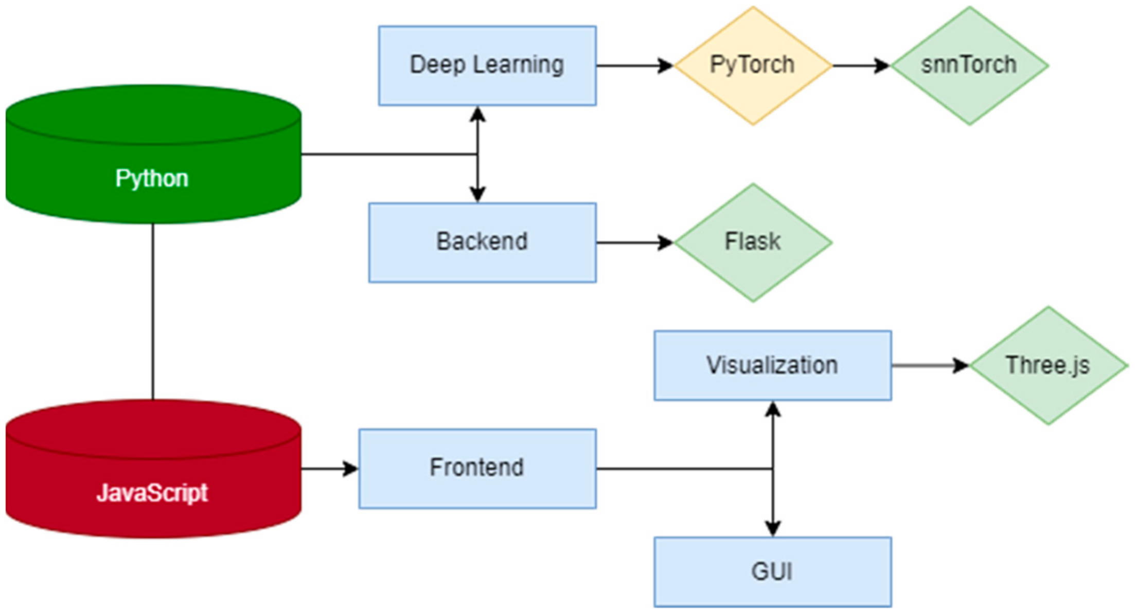
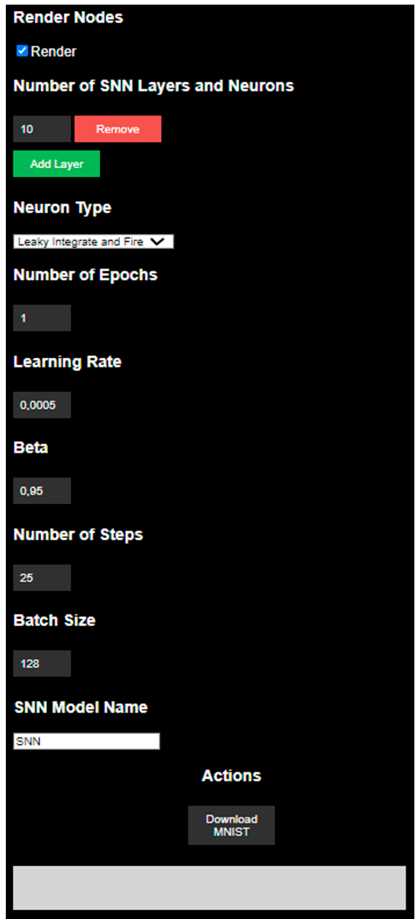
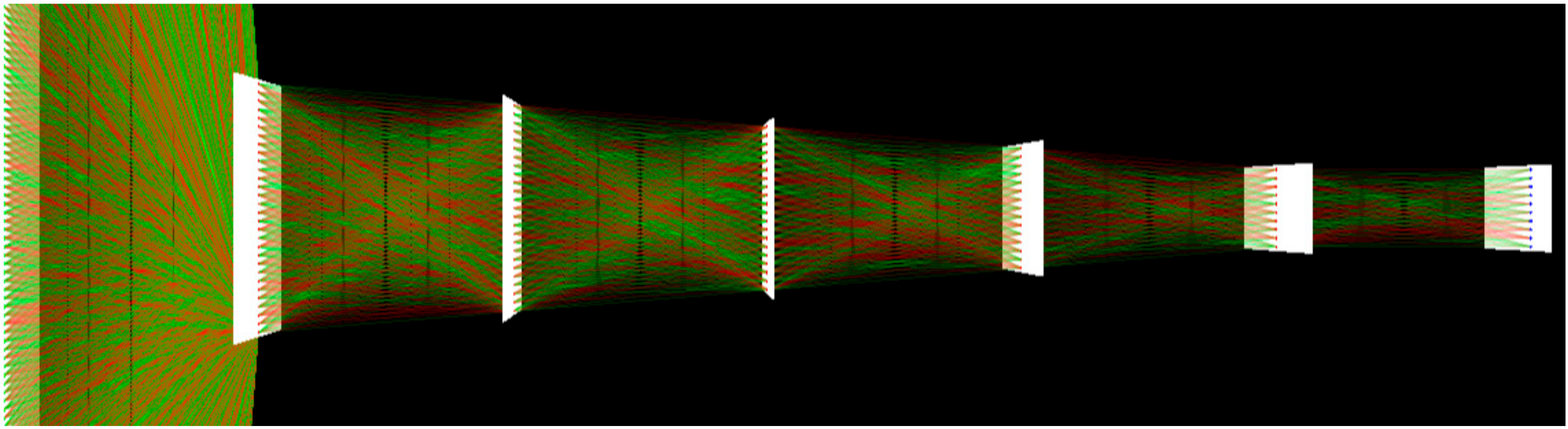
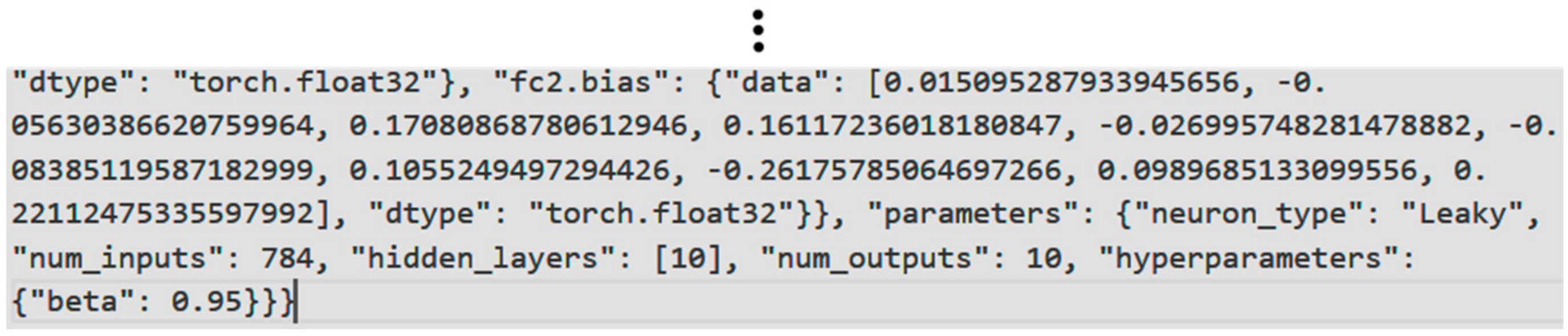
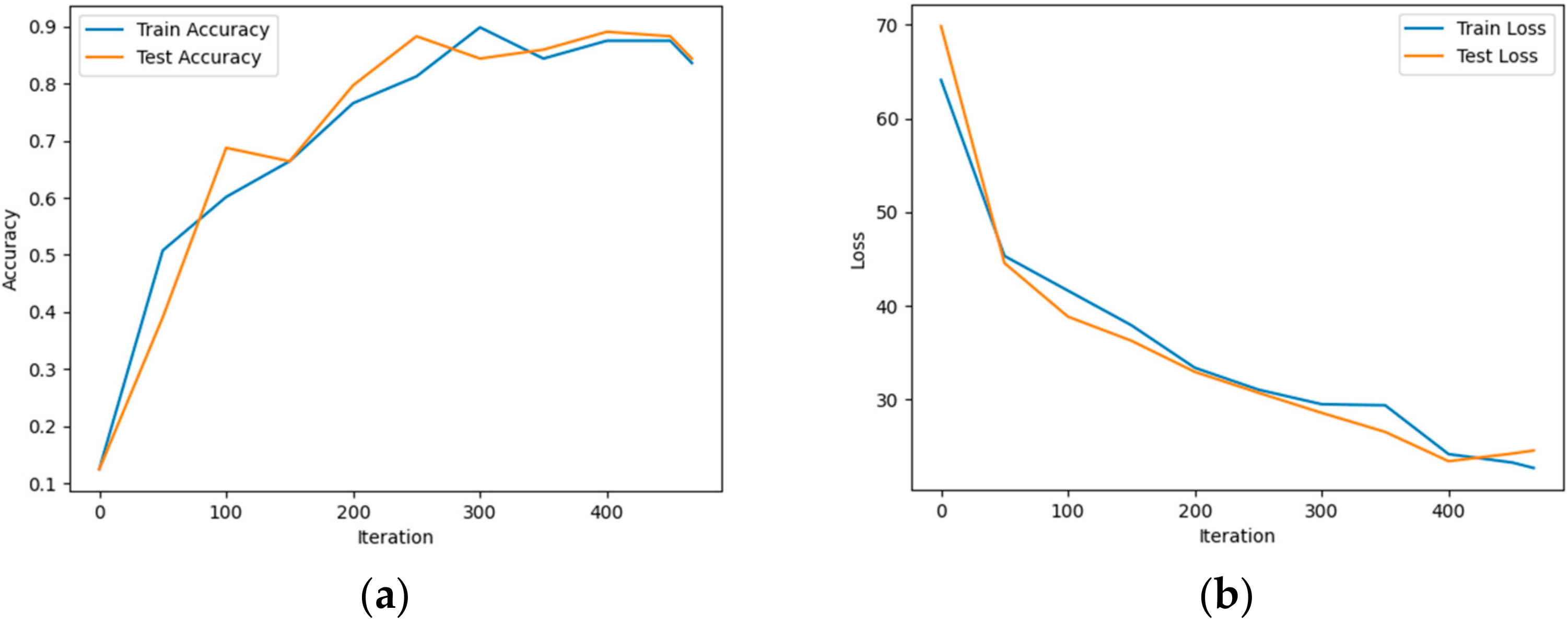
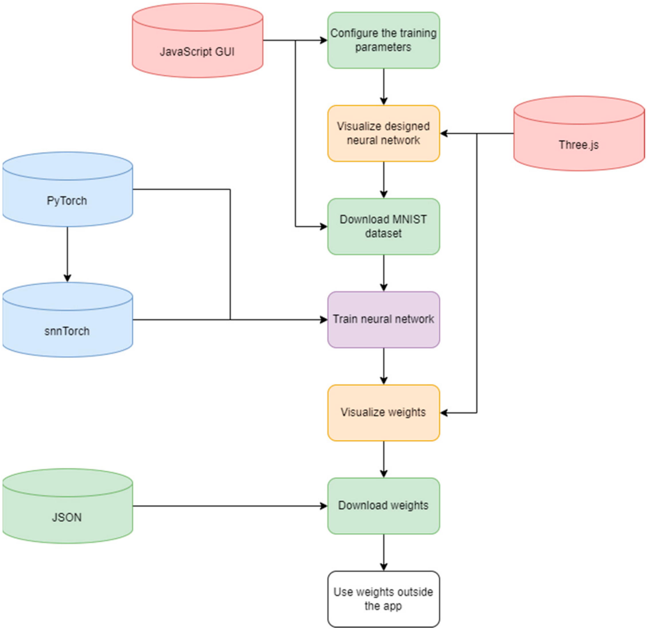
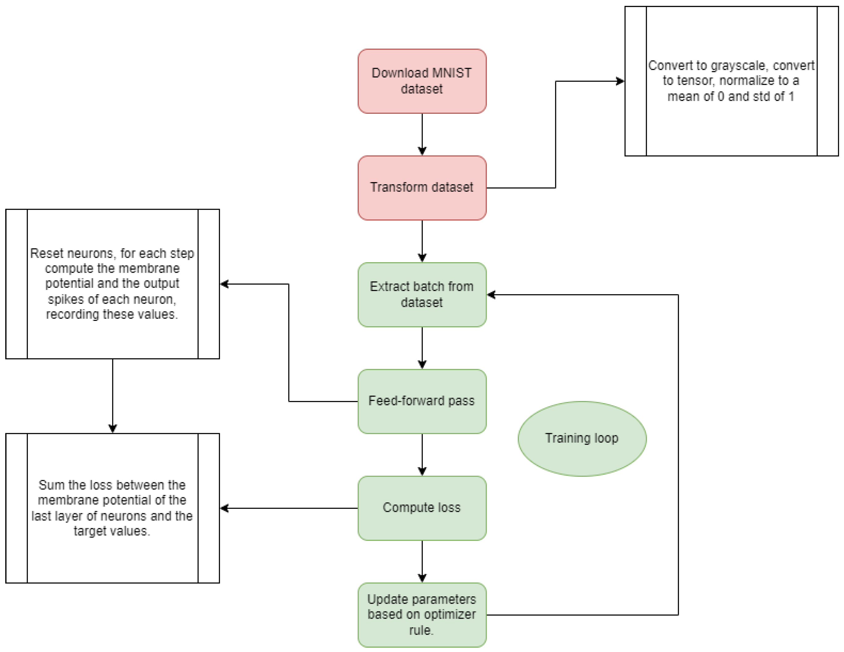
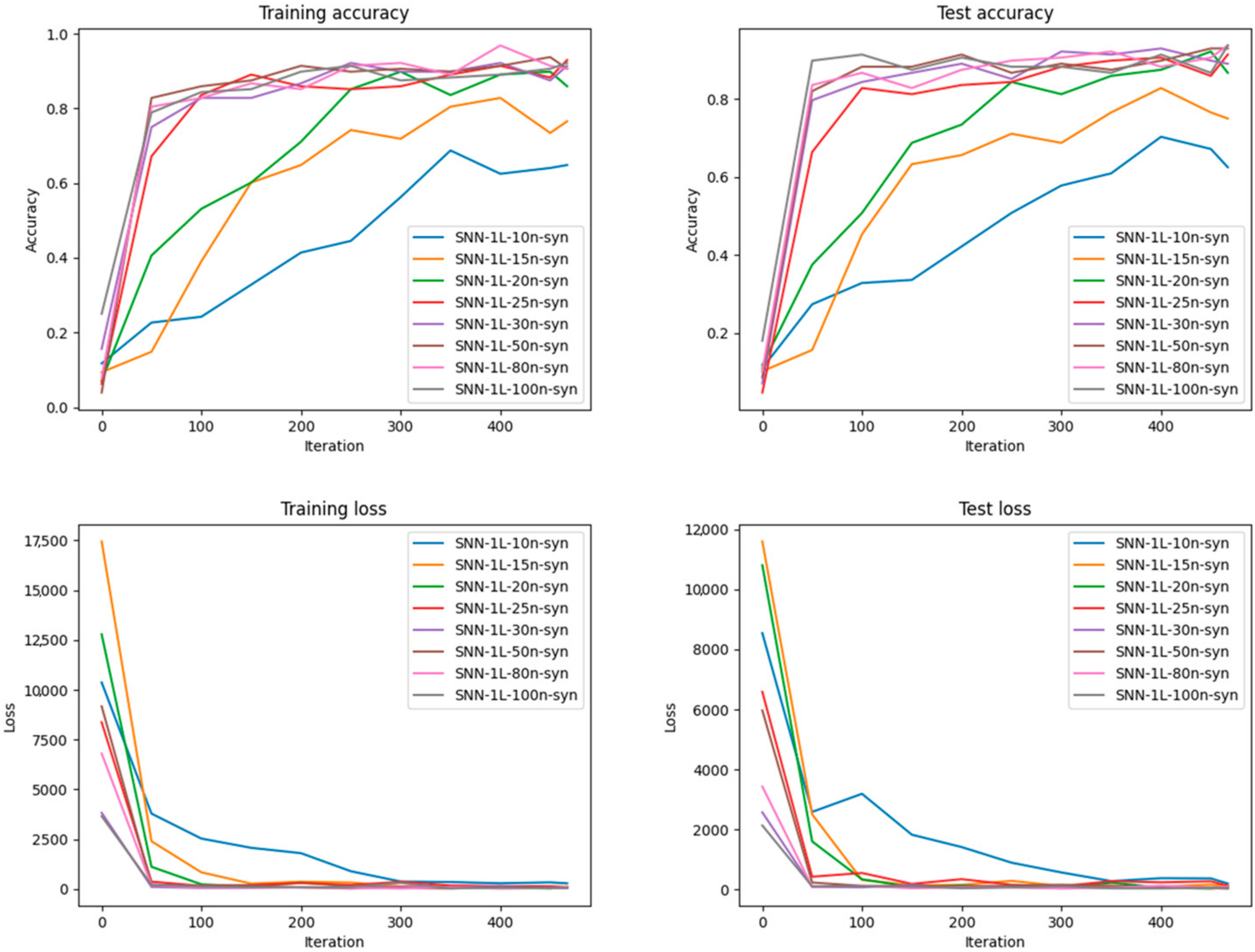
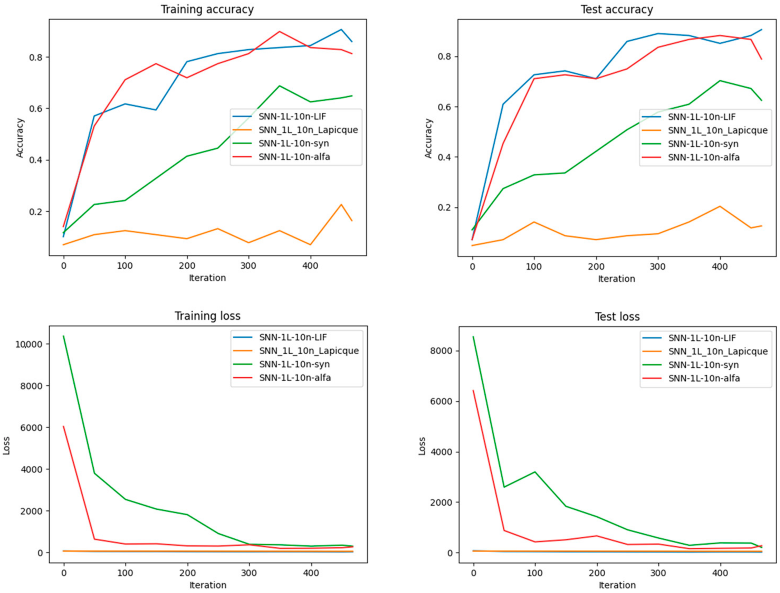
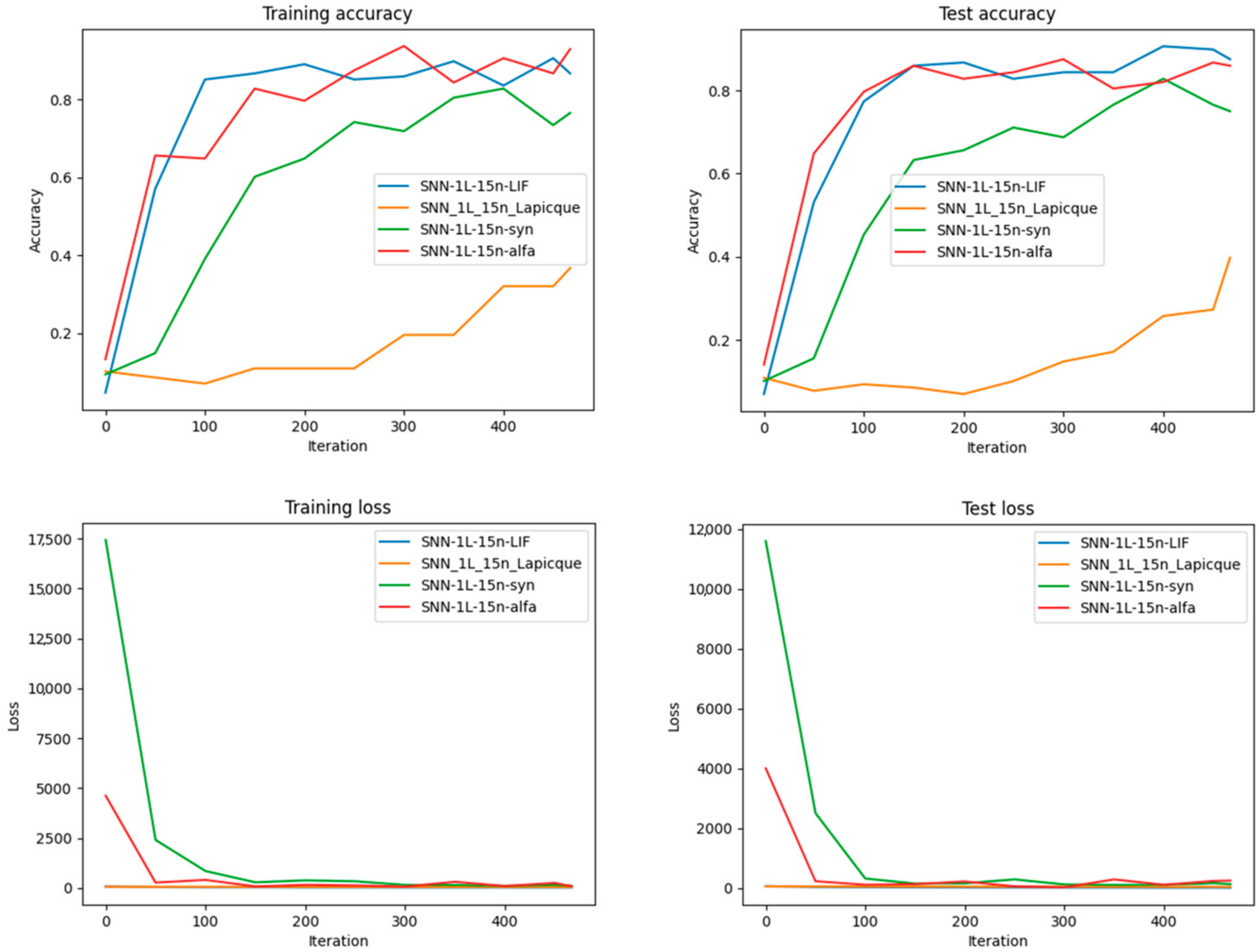
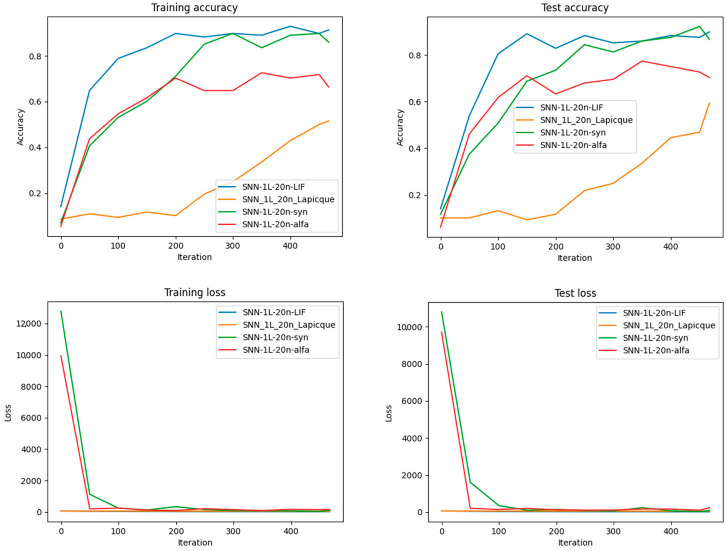
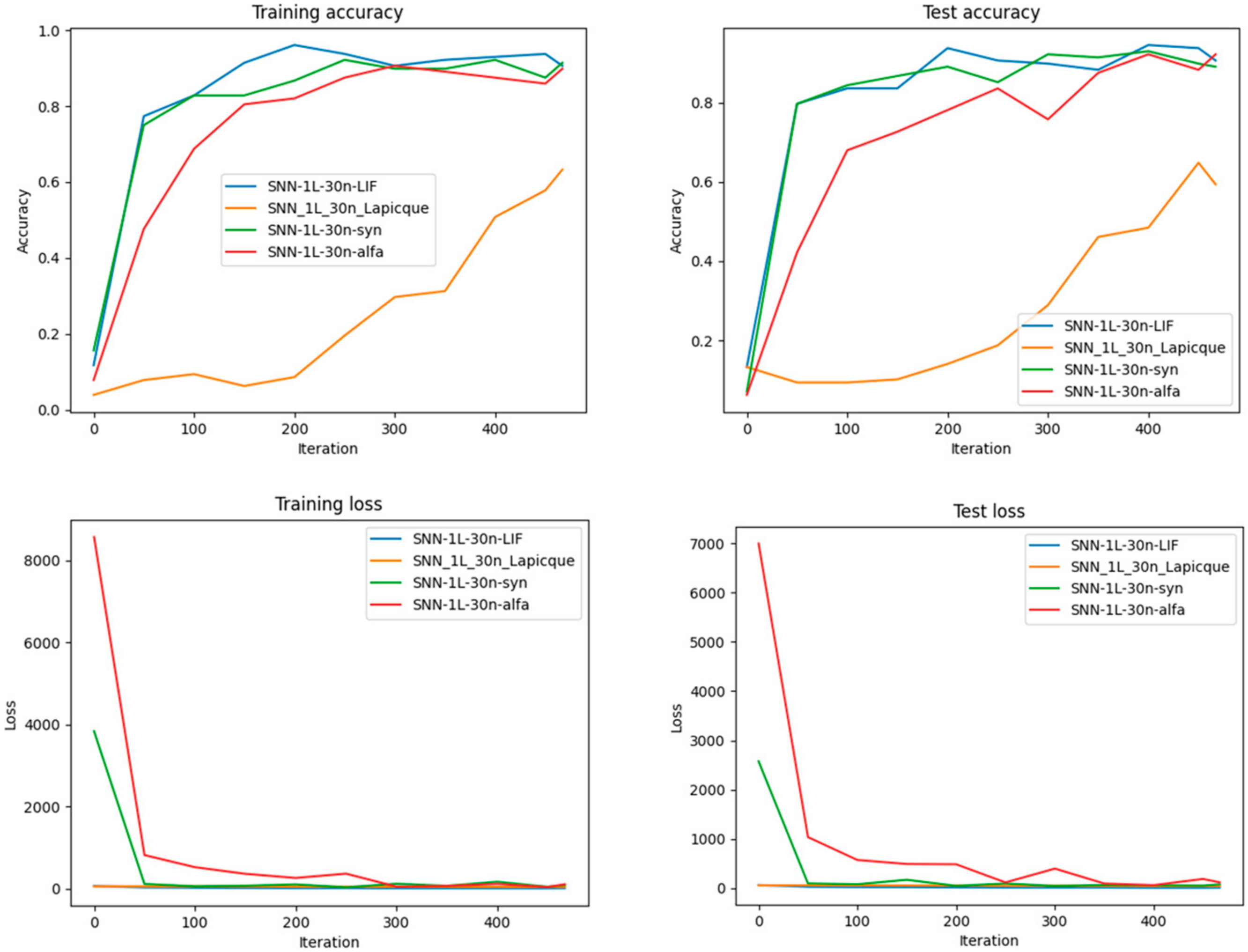
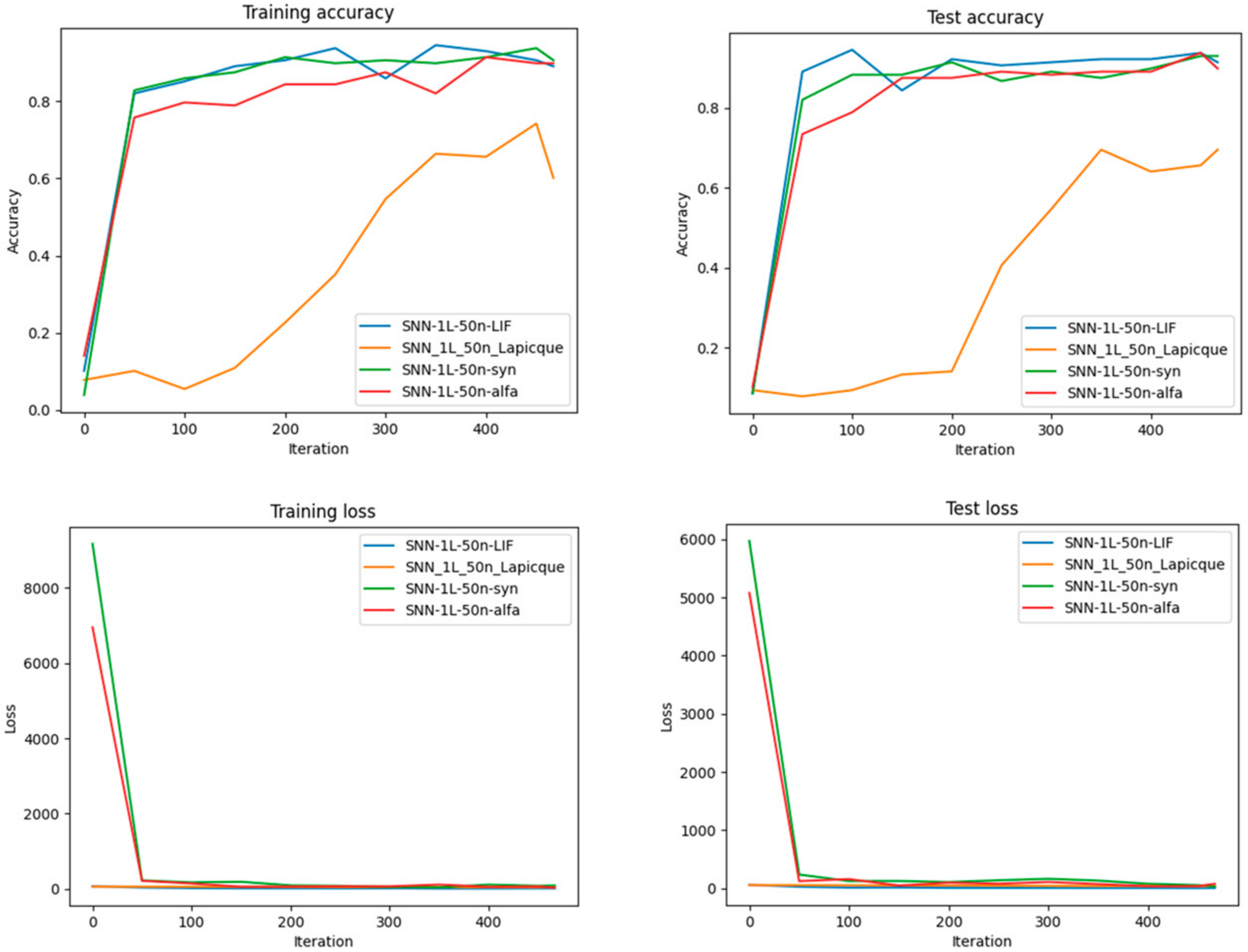